Open Access
Research
Anatomically based lower limb nerve model for electrical
stimulation
Juliana HK Kim*
1, John B Davidson
1, Oliver Röhrle
1, Tanya K Soboleva
3and
Andrew J Pullan
1,2Address: 1Bioengineering Institute, The University of Auckland, Private Bag 92019, Auckland, New Zealand, 2The Department of Engineering
Science, Faculty of Engineering, The University of Auckland, Private Bag 92019, Auckland, New Zealand and 3AgResearch Limited, Ruakura
Research Centre, Private Bag 3123, Hamilton, New Zealand
Email: Juliana HK Kim* - [email protected]; John B Davidson - [email protected]; Oliver Röhrle - [email protected]; Tanya K Soboleva - [email protected]; Andrew J Pullan - [email protected]
* Corresponding author
Abstract
Background: Functional Electrical Stimulation (FES) is a technique that aims to rehabilitate or restore functionality of skeletal muscles using external electrical stimulation. Despite the success achieved within the field of FES, there are still a number of questions that remain unanswered. One way of providing input to the answers is through the use of computational models.
Methods: This paper describes the development of an anatomically based computer model of the motor neurons in the lower limb of the human leg and shows how it can be used to simulate electrical signal propagation from the beginning of the sciatic nerve to a skeletal muscle. One-dimensional cubic Hermite finite elements were used to represent the major portions of the lower limb nerves. These elements were fit to data that had been digitised using images from the Visible Man project. Nerves smaller than approximately 1 mm could not be seen in the images, and thus a tree-branching algorithm was used to connect the ends of the fitted nerve model to the respective skeletal muscle. To simulate electrical propagation, a previously published mammalian nerve model was implemented and solved on the anatomically based nerve mesh using a finite difference method. The grid points for the finite difference method were derived from the fitted finite element mesh. By adjusting the tree-branching algorithm, it is possible to represent different levels of motor-unit recruitment.
Results: To illustrate the process of a propagating nerve stimulus to a muscle in detail, the above method was applied to the nerve tree that connects to the human semitendinosus muscle. A conduction velocity of 89.8 m/s was obtained for a 15 μm diameter nerve fibre. This signal was successfully propagated down the motor neurons to a selected group of motor units in the muscle.
Conclusion: An anatomically and physiologically based model of the posterior motor neurons in the human lower limb was developed. This model can be used to examine the effect of external stimulation on nerve and muscle activity, as may occur, for example, in the field of FES.
Published: 17 December 2007
BioMedical Engineering OnLine 2007, 6:48 doi:10.1186/1475-925X-6-48
Received: 30 July 2007 Accepted: 17 December 2007
This article is available from: http://www.biomedical-engineering-online.com/content/6/1/48
© 2007 Kim et al; licensee BioMed Central Ltd.
Background
Functional Electrical Stimulation (FES) is a technique, using external electrical stimulation, which is capable of rehabilitating or restoring functionality of skeletal mus-cles that has been paralysed, for instance, by central nerv-ous system lesions. The stimulation electrode can be located on the skin or implanted within the body to directly stimulate the muscles or nerves [1].
The direct stimulation of nerve trunks offers many advan-tages over transcutaneous or intramuscular stimulation. These advantages include the potential for controlling many muscles with a single implant, lower power require-ments and the ability to place the electrode far from the contracting muscles [2]. Also, further development on nerve electrodes, like FINE (flat interface nerve electrodes) [2], allow selective stimulation of fascicles in peripheral nerves, which could be important in selectively activating individual muscles as well as reducing muscle fatigue that often occurs with FES.
Despite the success of FES achieved to date, there are a number of questions that cannot yet be completely answered. For instance (i) how and where should the elec-trodes be arranged on the nerves to achieve a specific mus-cle response? (ii) what stimulation protocol should be used on a nerve to achieve a desired level of force while minimising the symptoms of muscle fatigue?
The answers to these questions strongly depend on how well one can predict the effects of external stimuli with respect to the initiation and propagation of nerve impulses within a nerve tree. An effective way of analysing such nerve responses is by appealing to a computational nerve model which is based on anatomical features and the electrophysiological behaviour of neurons.
Early nerve models used the Hodgkin-Huxley equations which are derived from experimental data on squid giant axons [3]. A decade later, Fankenhaeuser and Huxley developed a new model, the so-called Fankenhaeuser-Huxley (or FH) model that was based on experimental data from myelinated nerve fibres of the toad Xenopus laevis [4]. In 1976 McNeal developed the first nerve model for a myelinated fibre using stimulus electrodes outside a fibre. In 1985, the SENN model (Spatially Extended Nonlinear Node model), based on amphibian data, was presented by Reilly et al. [5]. This model can accommodate arbitrary spatial and temporal distributions of the extracellular potentials and thus it makes it possible to simulate the behaviour of myelinated nerve fibres for different extracellular electrode configurations and stimu-lus protocols. In 1987, Sweeney et al. [6] published the first model for warm blooded nerves using the data of Chiu et al. [7], which stem from myelinated nerves of
rab-bits. This model has subsequently been called the CRRSS model, named after the investigators Chiu, Ritchie, Rog-ert, Stagg and Sweeney. Schwarz and Eikhof also pre-sented their model, which was based on data from rat nerves [8]. In 1992, a modified SENN model was pre-sented by Frijns et al. [9]. This model has adapted the SENN model to fit mammalian nerve fibre data by taking into account the influence of body temperature on nerve kinetics. In 2001 McIntyre et al. [10] described a model of mammalian nerve fibres using the concept of a double cable that had been earlier proposed by Halt and Clark [11].
While all the above mentioned models have previously been used within the field of FES [12-15], the CRRSS model is by far most popular one. This nerve model describes mammalian nerves more realisticly than earlier ones and it does not require the use of a double cable structure. For all these reasons this paper uses the CRRSS model in order to examine signal propagation in an ana-tomically based representation of the nerves in the human lower limb.
To the authors' knowledge, none of the previous works within the field of FES have used an anatomically based geometry of the nerve tree in the lower limb. The geome-try of the nerve, however, plays a crucial role in analysing functional responses of muscles, e.g. the order of recruit-ment of muscles after an external source initiated a nerve stimulus. Therefore we have created an anatomically based geometric model of the posterior motor neurons in human lower limb to analyse the nerve responses more realistically and to allow us to look at the effect of external stimulation on nerve and muscle activity in the future.
Methods
Construction of the model of the lower limb nerves Anatomy
longus, flexor hallucis longus, fibular longus, fibular bravis, tibialis anterior, extenxor digitorum longus, and the extenxor hallucis longus.
Digitising and fitting of main nerve trunk
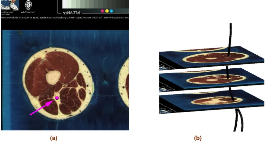
The main nerve trunk of the sciatic, tibial, common fibu-lar, deep fibular and superficial fibular nerves was created manually by digitising the images of the Visible Man (VM) dataset, which has a spatial resolution of 0.33 mm per pixel and 1 mm distance between slices [18]. The digitisa-tion was performed from slice VM0850 to VM1700. In cases where the main nerve trunk was not visible in the images, approximate locations of the nerves were identi-fied using standard anatomical texts e.g. [19]. Further-more, [20-22] were used to determine the location and the number of branches separating from the main nerve trunk to connect to a particular muscle. One-dimensional cubic Hermite finite elements were fitted to a point cloud, which was obtained by a manual digitisation process. The fitting process is described in [23,24]. The fitted nerve tree of the main trunk contains 145 elements. Figure 1 shows the VM slices used in the nerve digitisation process as well as part of the fitted model.
Nerve entry points
The biggest challenge in constructing a complete nerve tree from the images of the VM was the fact that nerves smaller than 1 mm cannot be identified. Hence an
algo-rithm needed to be developed that connects the main nerve trunk with the motor endplates of a muscle.
Motor endplates are the flattened ends of motor neurons that transmit neural impulses to a muscle. While the motor endplates cannot be determined directly from the VM images, their locations can be approximated using anatomical features specific to human skeletal muscle. In humans, muscle fibres run in most human leg muscles from tendon to tendon and the endplates are situated around the midpoint of the muscle fibre (the exceptions are the satorious and the gracillis muscles). Moreover, the innervating endplates form either a transverse band through the middle of the muscle or a concave endplate band depending on the shape of the specific muscle [25]. This is also true for the semitendinosus muscle which is separated into two areas by an internal tendon. Thus the semitendinosus muscle has two bands of motor endplates and two separate nerve branches leading to the muscle. Using the geometrical models of the muscles in the lower limb the nerve entry points can hence be computed by determining the middle points of muscle fibres that run from tendon to tendon.
The knowledge of the nerve entry points allowed the con-struction of the whole nerve model by means of a tree growing algorithm. The tree was constructed by connec-tion of two points to a single entity. This process is illus-trated in Figure 2. Note that the grouping of nerve entry
Digitising and fitting
Figure 1
points should depend on its association with a particular motor unit, which is the basic functional unit of a skeletal muscle. The number of fibres in a motor unit varies greatly, and can range from 6 to 2000 depending on the types of control necessary [26].
A detailed description of muscle motor units requires, for instance, a total of 580 motor units with 1720 fibres per motor unit for the gastrocnemius muscle or 445 motor units with 610 fibres per motor unit for the tibialis ante-rior muscle [26]. With this number of fibres and motor units a complete simulation of activation for the entire muscle is an extremely large computational job that is not currently feasible. However, individual skeletal muscle fibres are electrically isolated and the propagating action
potential is confined to single fibres. It is not thus neces-sary to include a detailed muscle fibre and motor unit description within our model to demonstrate the feasibil-ity of a whole nerve model. Therefore, a lower number (20–128) of motor units and one fibre per motor unit was used to generate the results shown below. This assump-tion, and the binary type nature of the tree constructed from nerve entry points, allow one to easily choose the number of active fibres within a muscle. We used a graded recruitment, which was consistent with the normal func-tioning of skeletal muscle. Here, we modelled the graded recruitment by selecting a certain percentage of motor unit points randomly out of the total motor units given in a muscle and connecting these points to the nerve tree. An illustration of this is given in Figure 3, which shows nerve
Motor unit recruitment
Figure 3
Motor unit recruitment. Generating nerve trees on the semimembranosus muscle from (a) 20 out of 20 motor entry points (100% recruitment). (b) 10 out of 20 motor entry points (50% recruitment) (c) 2 out of 20 motor entry points (10 % recruit-ment). A maximum of 20 motor units was used for illustrative purposes.
Connection to nerve entry points
Figure 2
trees for 100%, 50% and 10% recruitment of motor units in the semimembranosus muscle. For illustrative pur-poses only 20 motor units were depicted.
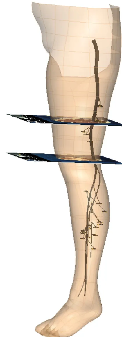
Figure 4 shows the completed nerve model inside the left lower limb with two of the VH images used in the model construction.
Signal propagation
Each fibre in a nerve is capable of generating an action potential which can be propagated along its length with-out loss of amplitude, duration, or velocity. The individ-ual fibres respond to stimulation according to the all-or-none principle: If the neuron does not reach the critical threshold level, then no action potential will be gener-ated. On the other hand, if the threshold level is reached, an action potential of a fixed size occurs.
For myelinated nerve fibres, axons are encased by Schwann cells which wrap a myelin sheath around the surface of the axon and have nodes of Ranvier which are regularly spaced along the axon. This is depicted in Figure 5(a) (reproduced from [27] with permission under GFDL). Since myelin sheaths provide insulation to the nerve, within the myelinated part of the nerve, action potentials can only be elicited at the nodes of Ranvier. Fig-ure 5(b) shows a simplified representation of the axon of a myelinated nerve by considering the axon as a cylinder with nodes of Ranvier at regular intervals along the cylin-der and with myelinated sheaths between the nodes of Ranvier.
As an axon reaches the vicinity of the skeletal muscle fibre it loses its myelin sheath [28]. The non-myelination and the small diameter of the nerve endings do both contrib-ute to the reduction of the conduction velocity by a factor of between 1/50 and 1/100 when compared to the speed at which the impulse travels in the myelinated unbranched parent axon [29]. In our model, however, the details of the nerve terminals were not modelled as the main focus of this study is on the conduction velocity of the unbranched axon. Hence, we assumed that the nerve fibre was myelinated along its entire length and the diam-eter of the fibre was constant along the whole nerve tree.
In the CRRSS model, the nodes of Ranvier are modeled by voltage-dependent sodium channels, voltage-independ-ent leakage channels and nodal capacitance. There are no voltage-dependent potassium channels in the ionic cur-rent equations of the CRRSS model since these channel types are scarce at nodes of Ranvier in mammalian myeli-nated nerve fibres. Hence action potential repolarization in mammalian myelinated axons is attributed to rapid sodium inactivation and a large leakage current [7]. A complete list of the CRRSS ionic currents equations
Completed nerve tree
Figure 4
together with the corresponding list of constants and var-iable names is given in APPENDIX A (See Additional file 1: appendixa).
With our proposed focus on external (extracellular) stim-ulation, the bidomain model was chosen to represent the electrical activity occurring along the nerve tree. The bido-main equations have the advantage that they explicitly model the extracellular potential and are given by
∇·((σi + σe) ∇φe) = -∇·(σi ∇Vm) + Istim, (1)
where
σi : intracellular conductance
σe : extracellular conductance
φe : extracellular potential
Vm : transmembrane potential
Iion : total ionic current, as given by the CRRSS model
Cm : membrane capacitance
Am : the ratio of membrane surface area to the volume
Istim :extracelluar injected current
To use the governing two bidomain equations to model myelinated fibres, the left hand side of the equation (2) needed to be multiplied by lm/ln [30]. Here, lm is a inter-nodal length (myelinated part) and ln is a nodal gap
length (node of Ranvier)(Figure 5(b)).
The modified bidomain equations were discretised using the same finite different scheme as proposed in [30]. The resulting equations were then solved using an implicit numerical integration scheme (LSODA) [31,32] with a uniform spatial discretisation and a fixed time step of 0.001 ms as implemented within CMISS [33]. Solving the modified bidomain equations with values as given in [6] resulted in a slow conduction velocity. Therefore, the value of the axoplasm resistivity, the ratio of fibre diame-ter to axon diamediame-ter and the ratio of indiame-ternodal length to axon diameter were changed in such a way that an appro-priate action potential conduction velocity for humans was generated. In Waxman's review [34] of the conduc-tion velocity in myelinated nerve fibres, he determined theoretically that to achieve maximal conduction velocity per axon diameter, the ratio of fibre diameter to axon diameter should be 0.6–0.7 and the ratio of the inter-nodal length to axon diameter was found to be 100–200. These ratios change for different nerves and species.
Guided by the work in [35], we set the ratio of axon diam-eter to fibre diamdiam-eter to be 0.67 and the ratio of inter-nodal length to axon diameter to be 200.
Signal propagation to a muscle fibre
To illustrate the process of a propagating nerve stimulus to a muscle in detail, the above method was applied to the nerve tree that connected to the human semitendinosus muscle. The bidomain model was also used to simulate electrical propagation within the muscle fibres. Here though, the CRRSS model was replaced by the muscle cell model [36].
The muscle model [36] is a mathematical model of a sin-gle skeletal muscle fibre that is based on electro-physio-logical processes. This model describes fast and slow twitch fibre types and was developed to investigate and model the muscle fatigue. The parameters that were used in our paper and deviated from [36] are listed in Table 1.
∇ ⋅ ∇ + ∇ ⋅ ∇ = ∂
∂ +
(σi Vm) (σ φi e) Am(Cm Vm ion),
t I
(2) Myelinated nerve and cable model
Figure 5
Results
We initially present results for the action potential propa-gation down the nerve tree. An initial cathodic extracellu-lar rectanguextracellu-lar current stimulus of 0.014 μA was imposed at a node at the beginning of the sciatic nerve for a dura-tion of 0.2 ms. The value of the current stimulus was obtained by injecting a 4.0 × 10⁴ μA/cm3 source over a 3.5
× 10-7 cm3 volume. Note that there is no distance between
the excitation monopolar electrode and the stimulated node. At this point in the nerve tree, the fibre diameter was set to be 15 μm based on [9], with a corresponding axon diameter of 10 μm and internodal length of 2.0 mm
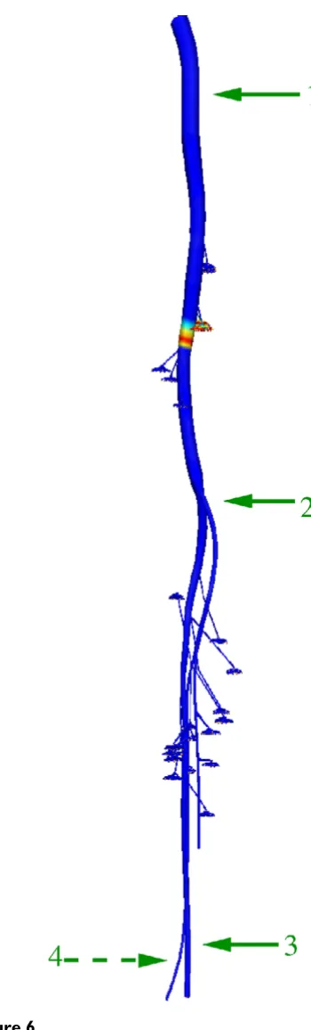
(since ratios of 0.67 and 200 had been set as discussed above). The axoplasm resistivity was set to be 0.24 Ohmm. Figures 6 and 7 depict the action potential propagation along the nerve tree. It can be seen that the computed action potentials at different positions along the nerves have the same shape, magnitude and duration. In our results, the magnitude of an action potential is approxi-mately 85 mV and its duration is 0.32 ms with a rise time 0.07 ms. This duration compares favourably with the known duration of an action potential at 37°C in the sin-gle myelinated rat nerve fibre (approximately 0.3 ms
[37]). Here, the calculation of the rise and fall times of the action potentials was done according to the method of [9].
The conduction velocity in the main nerve trunk was cal-culated by running the simulation for 10 ms and measur-ing the distance which the stimulus has propagated from a point close to the beginning of the sciatic nerve. The cal-culated conduction velocity was 89.8 m/s. This result agrees well with previously published theoretical results of 90 m/s [10,38]. It also agrees well with the experimental work of Boyd and Kalu [39], in which the relationship between conduction velocity and nerve fibre diameter was investigated experimentally using ten different muscle nerves in two cats.
In our work a conduction velocity of 85.35 m/s is pre-dicted from their approximate relationship.
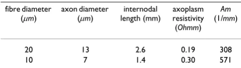
To further validate our model with respect to the calcu-lated conduction velocities, two further simulations, involving the parameters in Table 2, were considered. We
Action potential propagation
Figure 6
Action potential propagation. The entire nerve tree model. The coloured field between positions 1 and 2 repre-sent an action potential that has been generated from an extracellular stimulus at the top of the tree. Action potentials at positions labelled 1 through 4 are given in Figure 6. Table 1:
parameter nerve muscle description
Cm 2.5 1 capacitance/unit area(μF/cm2)
Ri(1/σi) 0.24 2.5 intracellular resistivity(Ohmm)
Re(1/σe) 0.24 1.11 extracellular resistivity(Ohmm)
chose 10 μm and 20 μm diameter fibres since the relation-ship between conduction velocities and fibre diameters investigated in [39] are between these two values. Axon diameters and internodal lengths are also chosen by the ratios we used for the 15 μm diameter fibre. For these parameters, our simulations predicted conduction veloci-ties 120 m/s and 54 m/s for the 20 μm and 10 μm diameter fibres respectively. In [38], the approximate conduction velocities are predicted to be 120 m/s for a 20 μm diameter fibre and 57 m/s for a 10 μm diameter fibre, where as [39] predicts conduction velocities of 113.8 m/s for a 20 μm
diameter fibre and 56.9 m/s for a 10 μm diameter fibre. In addition to the propagation of a nerve stimulus, we also simulated the resultant activity within the respective mus-cle. Figure 8 shows the semitendinosus muscle connected to the nerve tree. The signal propagation is illustrated in Figure 9, where an action potential was propagated along the nerve to initiate a contractile response within 128 muscle fibres embedded in the semitendinosus muscle. The semitendinosus muscle has an inscription in the mid-dle of the muscle and thus two branches of the nerve tree were connected to the upper and the lower part of the muscle. In Figure 9, the nerve model was stimulated at the beginning of the sciatic nerve and an action potential propagated along the nerve trunk, its branches, through
the motor endplates, and along the muscle fibres of the semitendinosus muscle.
Discussion
We have created an anatomically based geometric model of the posterior motor neurons of the human lower limb. The geometry was mainly based on data from the Visible Man dataset and was supplemented, where necessary, using existing anatomical and physiological texts. Using this geometrical representation, action potentials were simulated using a modified representation of the bido-main equations that incorporated the CRRSS ionic con-ductance model. When an appropriate external stimulus was applied, an action potential was propagated along the nerve tree with a constant velocity of 89.8 m/s for a 15 μm
diameter fibre. Most importantly the shape of an action potential was not altered by the simulation. The com-puted action potential conduction velocity agrees well with previously published theoretical and experimental estimates [10,38,39].
The axoplasm resistivity we used for the 15 μm diameter fibre was lower than that used in the original CRRSS model (0.24 Ohmm compared to 0.547 Ohmm [6]). How-ever, in the original CRRSS paper, an intracellular stimu-lus was used with a 10 μm diameter fibre. It has also been noted that resistivity values are difficult to determine experimentally and agreed values are not yet well estab-lished [40].
The amplitude of the computed action potential (85 mV) was lower that reported in [37] which is about 105 – 110
mV. However, it should be noted that the amplitudes from [37] are obtained using experimental data from rat
Table 2: Simulation parameters for the 10 and 20 μm diameter fibres.
fibre diameter (μm)
axon diameter (μm)
internodal length (mm)
axoplasm resistivity (Ohmm)
Am
(1/mm)
20 13 2.6 0.19 308
10 7 1.4 0.30 571
Action potentials
Figure 7
and cat nerves as a guide. One of the reasons for the dif-ferent amplitude between the published values and the one presented in this paper could be the sodium (Na) transient since the membrane potential of the neuron is greatly affected by Na rushing into the cell when voltage gated channels open. If there is less Na available outside the cell, the inward driving force is decreased, creating a smaller depolarisation. To examine this in more detail, we compared the Na Nernst potential ENa between our model and the model of Schwarz et al. [37]. In our case the value was 35.64 mV (which is the same as that used in the orig-inal CRRSS model) whereas the model of Schawrz et al. [37] used a value of 60 mV. Changing the Na Nernst potential to 55.64 mV in our model resulted in the action
potential amplitude reaching approximately 100 mV
together with an increased conduction velocity of 120 m/ s. An additional increase of the axoplasm resistivity to 0.32 Ohmm decreased the conduction velocity to 90 m/s
without any alteration to the action potential amplitude. Thus, the proposed model appears to be able to generate appropriate conduction velocities and action potential amplitudes using the axoplasm resistivity and Na Nernst potential. We note that currently good values for these parameters for the human motor nerves are not available.
One of the limitations of our model is the graded recruit-ment which was only mimicked by selecting a certain per-centage of motor units and generating a nerve tree based on the motor entry points within these motor units. In other words, a graded recruitment was not achieved by the different strength of stimuli but by specifying the number of motor units to recruit a priori. This limitation can be overcome by modelling the sciatic nerve as a bundle of nerve fibres. With such a representation, each nerve fibre would be only connected to a specified set of motor units and the activation of each nerve fibre could then be defined according to the strength of stimuli. With our sin-gle nerve model replaced by a nerve bundle we can then investigate the relationship between surface electrode placement, stimulation strength, duration and activation of nerve fibres within the fibre bundle. The question of what external electrode configuration is required to achieve activation of a particular group of nerve fibres can then begin to be addressed. We intend to investigate this approach soon.
We have further shown that the nerve model can be con-nected to a skeletal muscle fibre model using the semi-tendinosus muscle as an illustration. The (neuron) action potentials propagated along the nerve to initiate a con-tractile response within the muscle. A novel approach of effectively bridging the scales of the electrophysiological cellular behaviour and the mechanical response of a skel-etal muscle has been recently developed [41]. This combi-nation can be used as a powerful tool to investigate and Semitendinosus muscle fibres connected to nerve tree
Figure 8
answer open questions in the field of FES, e.g the use of specific stimulation protocols to achieve a desired move-ment or to delay the fatigue process.
Conclusion
This paper introduces an anatomically based geometric model of the posterior motor neurons in human lower limb based on data from the Visible Man dataset. Using this geometrical representation, action potentials were computed using a bidomain representation that incorpo-rated the published ionic conductance model. The results indicate that this model can be used to look at the effect of external stimulation on nerve and muscle activity in the field of FES.
Competing interests
The author(s) declare that they have no competing inter-ests.
Authors' contributions
Author JHKK created the human lower limb nerve model based on VH images, performed the various simulations required, analyzed the results and drafted the manuscript. Author JBD created the muscle fibres and connected it to the nerve model and performed simulations required. Author OR helped to create the semitendinosus muscle and revised the manuscript. Author TKS contributed to the muscle model development. Author AJP was actively involved in the supervision and development of the research and revised the manuscript. All authors read and approved the final version of the manuscript.
AP propagation to the semitendinosus muscle
Figure 9
Publish with BioMed Central and every scientist can read your work free of charge "BioMed Central will be the most significant development for disseminating the results of biomedical researc h in our lifetime."
Sir Paul Nurse, Cancer Research UK
Your research papers will be:
available free of charge to the entire biomedical community
peer reviewed and published immediately upon acceptance
cited in PubMed and archived on PubMed Central
yours — you keep the copyright
Submit your manuscript here:
http://www.biomedcentral.com/info/publishing_adv.asp
BioMedcentral
Additional material
Acknowledgements
Funding for this work is provided by the Foundation for Research Science and Technology (FRST) under contract number C10X0402.
References
1. Peripheral nerve and muscle stimulation [http:// www.case.edu/groups/ANCL/pages/99/Ch4-2-Preprint.pdf] 2. Leventhal D, Durand D: Subfascicle stimulation selectivity with
the flat interface nerve electrode. Annals of Biomedical Enginering
2003, 31:643-652.
3. Hodgkin A, Huxley A: A quantitative description of membrane current and its application to conduction and excitation in nerve. The Journal of Physiology 1952, 117:500-544.
4. Frankenhaeuser B, Huxley A: The action potential in the myeli-nated nerve fibre of xenopus laevis as computed on the basis of voltage clamp data. The Journal of Physiology 1964, 171:302-315. 5. Reilly J, Freeman V, Larkin W: Sensory effects of transient elec-trical stimulation evaluation with a neuroelectric model.
IEEE Transactions on Biomedical Engineering 1985, 32:1001-1011. 6. Sweeney J, Mortimer J, Durand D: Modelling of mammalian
mye-linated nerve for functional neuromuscular stimulation. IEEE 9th Annual Conference of the Engineering in Medicine and Biology Society
1987:1577-1578.
7. Chiu S, Ritchie J, Rogart R, Stagg D: A quantitative description of membrane currents in rabbit myelinated nerve. The Journal of Physiology 1979, 292:149-166.
8. Rattay F, Aberham M: Modeling Axon membranes for func-tional electrical stimulation. IEEE Transactions on Biomedical Engi-neering 1993, 40:1201-1209.
9. Frijins J, Mooij J, ten Kate J: A quantitative approach to modeling mammalian myelinated nerve fibers for electrical prosthesis design. IEEE Transactions on Biomedical Engineering 1994, 41:556-566. 10. McIntyre C, Richardson A, Grill W: Modeling the excitability of mammalian nerve fibers:influence of afterpotentials on the recovery cycle. J Neurophysiol 2001, 87(2):995-1006.
11. Halter J, Clark J: A distributed-parameter model of the myeli-nated nerve fiber. Journal of Theoretical Biology 1991, 148:345-382. 12. Litvak L, Delqutte B, Eddington D: Auditory nerve fiber responses to electric stimulation: modulated and unmodu-lated pulse trains. The Journal of the Acoustical Society of America
2001, 110:368-379.
13. Mahnam A, Firoozabadi S, Hashemi S, Janahmadi M: The use of ramp-shaped stimulus waveform for selective stimulation of neural fibers in peripheral nerves. The 2nd European Biomedical Engineering Conference EMBEC 05 2005 .
14. Struijk J, Holsheimer J, van der Heide G, Boom H: Recruitment of dorsal column fibres in spinal cord stimulation: influence of collateral branching. IEEE Transactions on Biomedical Engineering
1992, 9:903-912.
15. Colombo J, Parkins C: A model of electrical excitation of the mammalian auditory-nerve neuron. Hearing Research 1987, 31:287-311.
16. Williams P, (Ed): Gray's anatomy Churchill Livingstone; 1995. 17. Agur A, Lee M: Grant's atlas of anatomy Lippincott Williams & Wilkins;
1999.
18. Spitzer V, Ackerman M, Scherzinger A, Whitlock D: The visible human male: a technical report. J of the American Med Informatics Ass 1996, 3(2):118-130.
19. Eycleshymer A, Schoemaker D: A cross-section anatomy London:But-terworths; 1970.
20. Woodley S, Mercer S: Hamstring muscles: architecture and innervation. Cells Tissues Organs 2005, 179:125-141.
21. Sunderland S, Hughes E: Medical and non-medical features of the muscular branches of the sciatic nerve and its medial and lateral popliteal divisions. The Journal of Comparative Neurology
1946, 85:205-222.
22. Blyth P: Modelling the nerves of the lower limb. Tech. rep., Department of bioengineering science, University of Auckland; 2001. 23. Bradley C, Pullan A, Hunter P: Geometric modeling of the human torso. Annals of Biomedical Engineering 1997, 27(1):96-111. 24. Fernandez J, Mithraratne P, Thrupp S, Tawhai M, Hunter P:
Anatom-ically based geometric modelling of the musculo-skeletal sys-tem and other organs. Journal Biomechanics and Modeling in Mechanobiology 2004, 2:139-155.
25. Aquilonius S, Asknark H, Gillberg P, Nandedkar S, Olsson Y, Stalberg E: Topographial localization of motor endplates in cryosec-tions of whole human muscles. Muscle & Nerve 1984, 7:287-293. 26. Guyton A: Textbook of medical physiology Philadelphia; London,
Saun-ders; 1986.
27. Neuron-no labels.png [http://en.wikipedia.org/wiki/Image:Neu ron-no_labels.png]
28. Gartner L, Hiatt J: Color atlas of histology Lippincott Williams & Wilkins; 2006.
29. Katz B, Miledi R: Propagation of electric activity in motor nerve terminals. Proceedings of the Royal Society of London, Series B, Biological Sciences 1965, 161:453-482.
30. Rattay F: Analysis of models for external stimulation of axons.
IEEE Transactions on Biomedical Engineering 1986, 33:974-977. 31. Hindmarsh A: ODEPACK, "A systematized collection of ODE solvers", in
scientific computing North-Holland, Amsterdam; 1982.
32. Petzold L: Automatic selection of methods for solving stiff and nonstiff systems of ordinary differential equations. SIAM Jour-nal on Scientific Computing 1983, 4:136-148.
33. CMISS [http://www.cmiss.org]
34. Waxman S: Determinants of conduction velocity in myeli-nated nerve fibers. Muscle & Nerve 1980, 3:141-150.
35. Reinard L, Bischhausen R: How are sheath dimensions affected by axon caliber and internode length? Brain Research 1982, 235:335-350.
36. Shorten P, O'Callaghan P, Davidson J, Soboleva T: A mathematical model of fatigue in skeletal muscle force contraction. J Muscle Res Cell Motil 2007 in press.
37. Schwarz J, Eikhof G: Na currents and action potentials in rat myelinated nerve fibers at 20 and 37°C. Pflgers Archiv European Journal of Physiology 1987, 409:569-577.
38. Rushton W: A theory of the effects of fiber size in medullated nerve. The Journal of Physiology 1951, 115:101-122.
39. Boyd I, Kalu K: Scaling factor relating conduction velocity and diameter for myelinated afferent nerve fibers in the cat hind limb. The Journal of Physiology 1979, 289:277-297.
40. Wesselink W, Holsheimer J, Sönmez Z, Boom H: A simulation model of the electrical characteristics of human myelinated sensory nerve fibers. Med Biol Eng Comput 1997, 37(2):2028-2035. 41. Röhrle O, Davidson J, Pullan A: Bridging scales: a three-dimen-sional electromechanical finite element model of skeletal muscle. SIAM Journal on Scientific Computing 2007 in press.
Additional file 1
APPENDIX A. The equations, variables and constants used in our model are presented.
Click here for file