P R O C E E D I N G S
Open Access
A novel method for the normalization of
microRNA RT-PCR data
Rehman Qureshi, Ahmet Sacan
*From
The 2011 International Conference on Bioinformatics and Computational Biology (BIOCOMP
’
11)
Las Vegas, NV, USA. 18-21 July 2011
Abstract
Background:MicroRNAs (miRNAs) are short non-coding RNA molecules that regulate mRNA transcript levels and
translation. Deregulation of microRNAs is indicated in a number of diseases and microRNAs are seen as a
promising target for biomarker identification and drug development. miRNA expression is commonly measured by microarray or real-time polymerase chain reaction (RT-PCR). The findings of RT-PCR data are highly dependent on the normalization techniques used during preprocessing of the Cycle Threshold readings from RT-PCR. Some of the commonly used endogenous controls themselves have been discovered to be differentially expressed in various conditions such as cancer, making them inappropriate internal controls.
Methods:We demonstrate that RT-PCR data contains a systematic bias resulting in large variations in the Cycle Threshold (CT) values of the low-abundant miRNA samples. We propose a new data normalization method that considers all available microRNAs as endogenous controls. A weighted normalization approach is utilized to allow contribution from all microRNAs, weighted by their empirical stability.
Results:The systematic bias in RT-PCR data is illustrated on a microRNA dataset obtained from primary cutaneous melanocytic neoplasms. We show that through a single control parameter, this method is able to emulate other commonly used normalization methods and thus provides a more general approach. We explore the consistency of RT-PCR expression data with microarray expression by utilizing a dataset where both RT-PCR and microarray profiling data is available for the same miRNA samples.
Conclusions:A weighted normalization method allows the contribution of all of the miRNAs, whether they are highly abundant or have low expression levels. Our findings further suggest that the normalization of a particular miRNA should rely on only miRNAs that have comparable expression levels.
microRNA RT-PCR, Normalization, Microarray
Background
MicroRNAs (miRNAs) are short non-coding RNA sequences that average 22 nucleotides in length [1-3]. This class of RNAs is distinct from other short sequence RNA types such as siRNA and snRNA. The first RNA of this class was identified in C. Elegans in 1993 [4]. How-ever, miRNAs were not recognized as a special class of RNAs until a decade ago [5]. To date, all animal and plant species have been found to express miRNAs [6]. At
this time approximately 1000 miRNA sequences have been identified in the human microribonucleome [7]. miRNA sequences are highly evolutionarily conserved among mammals [4,8-12]. Approximately 80% of known miRNA genes are found in intronic regions of the gen-ome [13,14]. miRNAs are involved in many biological processes by influencing the regulation of specific target genes, generally resulting in the down-regulation of those target genes. There are two postulated methods by which miRNAs act on their target genes. If the miRNA binds with an mRNA transcript and they exhibit high comple-mentarity, it will cause the degradation of the mRNA. If the miRNA binds with incomplete complementarity then * Correspondence: [email protected]
Center for integrated Bioinformatics, School of Biomedical Engineering, Science and Health System, Drexel University, 3120 Market Street, Philadelphia, PA 19104, USA
it causes translational repression of the mRNA. In plants the primary mechanism of action of miRNAs is mRNA transcript degradation, while in animals, translational repression is more common [6]. An estimated 60% of mammalian mRNAs are targeted by one or more miR-NAs [10,12].
miRNAs have been discovered to play a role in many diseases and pathologies [2,10,13,15,16]. The role of miR-NAs in cancer has been examined and several miRmiR-NAs have been found to regulate tumor-related genes [1-3,10,13,17-19]. In fact, more than half of all miRNA genes are located in cancer-associated regions of the gen-ome or in fragile sites [3,13]. As a result, therapeutic applications of miRNAs are being investigated. Further-more, due to the link between many miRNAs and cancer, these RNA molecules are being investigated as potential cancer biomarkers. The fact that some miRNAs can be found extracellularly and maintain their stability in the extracellular environment facilitates their usage as bio-markers [10].
There are two main tools used to quantify the expres-sion of miRNAs: microarrays and real-time polymerase chain reaction (RT-PCR). RT-PCR returns the number of cycles that the samples underwent before they were detected, reported as a value known as the Cycle Thresh-old (CT). The CT values vary logarithmically with expres-sion levels. There are several methods of normalizing the data and calculating the fold-change of each gene between samples. For convenience, in this presentation the terms,
“miRNA”and“gene,”are used interchangeably in the con-text of RT-PCR.ΔCT values are calculated by subtracting the CT value of the endogenous control for a given sample (or the mean of the CT values of the endogenous controls if more than one exist) from the CT value of the gene for the given sample. In the calculation ofΔCT values we refer to the number subtracted from the raw CT values of each gene as theCT0. TheΔΔCT is calculated by subtract-ing theΔCT of an experimental sample from a control sample. Fold change is calculated by raising 2 to the power of the negativeΔΔCT value, since CT values are related to the amount of miRNA or gene logarithmically [20]. The relationship between CT,ΔCT,ΔΔCT, and Fold Change (FC) are given by the equations below.
CT=CT−CT0 (1)
ΔΔCT=ΔCT−ΔCTcontrol (2)
FC= 2−ΔΔCT (3)
Theoretically, endogenous controls are selected because they have low variance in their expression levels across samples. In the case of miRNAs, the endogenous controls are typically recommended by the manufacturer
of the miRNA kit used in the PCR. Some of the most commonly used endogenous controls are RNU44, RNU48, and U6 [17]. However, the usage of these endo-genous controls is problematic, because even though these endogenous controls have stable expression levels in normal tissue samples, they have been found to be dif-ferentially expressed in cancerous tissue compared with normal tissue [20].
Directly applying this method can lead to misleading results if the CT values in the data are not normalized. There are several commonly used methods for miRNA normalization, including: quantile normalization, median normalization, and cyclic loess. Quantile normalization involves sorting the expression values of each gene in a given sample in order from least to greatest. This is done for each sample in the study. The vectors of the sorted CT values for each sample are combined into a matrix. The mean of each row of the matrix is calculated. The CT value in each element in each row is replaced with the mean of the entire row. In the case of median quan-tile normalization the median of the row is used instead of the mean. The CT values in each sample are then rear-ranged back into their original order. This causes the dis-tribution of CT values across all samples to assume the same shape, which will minimize the variance except for that resulting from the experimental condition beings studied [21,22].
Median normalization shifts the CT values in each sample such that the median CT value of each sample is the same. The median of each plate should be deter-mined, and the medians of all plates should be arranged in a vector and sorted to determine the median of the medians. In each plate the difference between the median of the sample and the overall median should be sub-tracted from the CT value of each gene [9].
In cyclic loess normalization, pairs of plates are consid-ered. For all pairs of plates the difference of the log of the CT for each gene is represented byM, and the average of each gene of the log of the expression values is repre-sented byA. Then a loess curve is fit by regression ofM onAwhich results in a fitting vectorF. The genes in the first sample are adjusted by adding half theFvalue corre-sponding to the log of the CT for each gene. In the second sample half theFvalue is subtracted from the log CT of the gene [9,21].
set normalization [24]. In rank-invariant set normaliza-tion genes are ranked by their expression for each sam-ple and the ranked list is compared to the ranked list of genes for a reference sample. Genes are considered to be rank-invariant if they have similar ranks in the refer-ence sample and the experimental sample. All experi-mental samples are compared to the reference sample and an intersection of these lists is used to identify the rank-invariant genes which can then be used for nor-malization [24]. Deo et al. compared several normaliza-tion methods and concluded that data-driven methods performed best. They compared normalization by endo-genous controls, using the mean as a pseudo-control, and two different methods of quantile normalization. They concluded that quantile normalization performed the best despite the fact that using the mean as an endogenous control produced lower standard deviation [23].
One of the main problems with RT-PCR that remains as yet unaddressed by current normalization methods is the systematic bias present within the data. We observe that standard deviation increases as CT values increase. We believe that the most likely cause of this observation is the assumption that the PCR magnifica-tion at each cycle is an exact doubling of the expres-sion levels is inaccurate. There seems to be an accumulation of an expression-level specific rate-limit-ing effect. As a result, a small difference in the size of the initial sample being amplified causes larger varia-tions in the CT values of the less abundant microRNA molecules. Consequently, using endogenous controls, which are usually chosen from highly expressed micro-RNAs, for normalization becomes inappropriate for the less-abundant microRNAs. Even quantile normalization has been observed to produce more variance at high CT values than was present in the original raw data [24]. One potential solution is to use the mean expres-sion values of all genes in a sample as the endogenous control, as proposed by Mestdagh et al. [15], and calcu-lateΔCT by subtracting this mean CT value from the CT value of all genes in the sample. However, this approach is not ideal because the mean of the entire sample is sensitive to fluctuating genes as well as unde-tected genes which have high CT values. As a result, the mean-value normalization method is dominated by the large fluctuations of the less-abundant microRNAs and may cause spurious differential expression levels for otherwise stable microRNAs. In this study, we pro-pose a method of using a weighted mean as an artificial endogenous control to calculateΔCT values. The stan-dard deviation of a microRNA across all samples is considered as a stability measure and each microRNA is weighted by its stability to generate the artificial endogenous control levels.
Methods
The primary dataset used in this study was obtained from a recently deposited microRNA RT-PCR dataset in the Gene Expression Omnibus (GEO) [25]. The data was from a study by Jukic et al. that examined the dif-ference in miRNA expression profiles in melanocytic neoplasms between young and older adults [1]. Their study examined 10 young adults and 10 older adults and measured the expression of 666 microRNAs. We used the raw CT values measured in their data to com-pare different approaches to normalizing the data. This dataset has been previously used by Deo et al. to com-pare various normalization techniques; this dataset is highly suited to the comparison of normalization studies due to the large number of samples and the use of mul-tiple cards [23].
We have investigated several normalization methods, including quantile, mean, and median normalization methods, and endogenous controls identified using var-ious stability criteria. In mean and median normaliza-tion, the mean and median of all of the genes in a given sample are used as the value forCT0. For identification of endogenous controls, we calculate the standard devia-tion of each microRNA across all samples, and rank them in the order of increasing standard deviation. The CT values of the top-kmicroRNAs are averaged in each sample to provide theCT0values.
A new weighted mean metric is proposed using the standard deviations of the microRNAs as weights. For a given gene, the weighted average is calculated using the following equation:
CT0=
n
j CTj×
1 STDCTj
wmp
n
i=11/STD(CTi)
(4)
wherewmpis the weighted mean power, which can be adjusted to shift the dominance between stable and unstable microRNAs, n is the number of genes or microRNAs, and STD is a function that returns the standard deviation. The weighted mean calculation involves raising the inverse of the standard deviation of a given gene across all samples to the weighted mean power, which is usually specified as 1, and dividing by the sum of the inverses of the standard deviations for all genes.CT0 is calculated for each sample by taking the sum of the product of all the raw CT values in the sam-ple and the previous number. When the ΔCT is calcu-lated the CT of each gene is subtracted by the above value. This method gives a higher weight to genes with a lower standard deviation.
To explore this topic we utilized data from Chen et al. [26]. They evaluated miRNA expression in murine myo-blasts utilizing both RT-PCR and microarrays. They evalu-ated the consistency of different RNA preparation methods for RT-PCR. We harnessed their data to explore the correlation of RT-PCR with microarray. We further explored whether the expression level of a particular miRNA in RT-PCR would bias its correlation with its expression on a microarray.
Results and Discussion
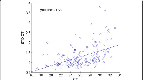
In order to test the hypothesis that increasing CT values magnifies the natural variation between the initial amounts of samples loaded in each well during RT-PCR, we exam-ined the standard deviation of the genes against their mean CT values, as shown in Figure 1. The application of linear regression to this data clearly shows a trend of increasing standard deviation values for higher CT values. Note that the higher the CT value, the more cycles were required to observe that microRNA, hence the less abun-dant that microRNA was in the initial loaded sample.
As expected, the CT values of most genes are well corre-lated with the mean expression of all the genes. This is illustrated in Figure 2, where we show the expression of the 20 miRNAs that are most correlated with the mean expression. Each tick on the x-axis represents a unique experimental sample.
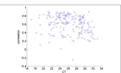
The correlation with the mean expression level extends to low-abundant miRNAs. We demonstrate this in Figure 3, wherein the Pearson correlation coefficient of the fluc-tuations in each gene with respect to its own average is shown against the fluctuations of the mean expression levels of all genes. The plot shows that a high correlation is observed whether the mean CT values are low or high.
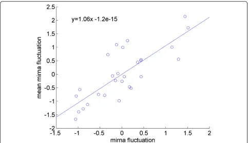
In order to quantify the sensitivity of the microRNA expression levels to the initial loaded sample size, a regres-sion line is fitted to the fluctuation of each miRNA against the fluctuation of mean expression. Fluctuation is deter-mined by subtracting the value of the expression of a miRNA in a given sample from the mean expression of that miRNA for all samples; the overall mean of the expression of all miRNAs in all samples can be subtracted from the sample means to determine the fluctuation of a sample mean. In Figure 4 we demonstrated this for a sin-gle miRNA. The x-value of each point is the difference between a sample mean and the overall mean, and the y-value is the difference between the expression of that par-ticular miRNA in that sample and the mean expression of that miRNA across all samples. The slope of the line indi-cates how sensitive the miRNA is to initial sample size, with larger slope values corresponding to larger variations in response to a small change in sample size. The slopes were calculated for all miRNAs. Figure 5 shows the sensi-tivity of each miRNA, which is determined by the slope
Figure 2miRNAs most correlated with the mean expression value. The CT values of 20 miRNAs where the change between samples is most correlated with the change in the mean expression value from sample to sample.
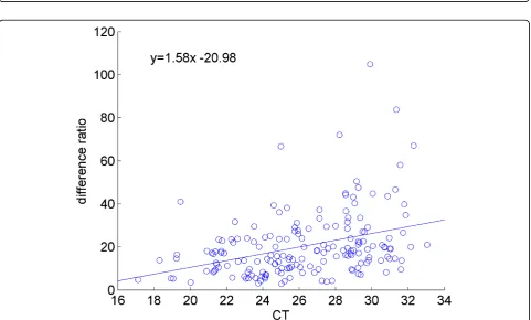
calculation demonstrated in Figure 4, versus against the overall mean expression level of that miRNA. We observe that the sensitivity is expression level dependent. Highly expressed miRNAs (those with small CT values) are less responsive to changes in the overall mean of the miRNAs, whereas the low-abundant genes are more sensitive to the changes in the overall mean of the miRNAs. Note that, this is not simply a random effect due to low abundant microRNAs being more variable, since the variation is still correlated and is in the same direction of the change in mean expression level. The same observation is made by examining the ratio of the fluctuations in individual miR-NAs to the fluctuations of the mean expression level, as shown in Figure 6.
In conclusion, the fluctuations of the low-abundant miRNAs are not random. The changes in their expres-sion levels are correlated well with the overall changes in all miRNAs, which is assumed to be due to different starting sample sizes for the PCR reactions. We see that there is a systematic bias in the CT values that causes the expression levels of the low-abundant miRNAs to be more sensitive to the initial sample sizes.
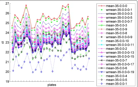
We then investigated the suitability of our weighted mean metric. In Figure 7 we display the values forCT0 for several different methods including using the mean of
all raw CT values in the bottom line (top-k= 0), the means of the top-kmiRNAs for different values ofk, and the weighted mean for different values for the weighted mean power. The plot demonstrates that varying the weighted mean power enables the shifting of the curve upwards or downwards. In Table 1 and Table 2, we com-pare the resulting means, standard deviations, and geN-orm stability values [27] for mean and weighted mean normalizations, respectively. We repeat analysis this for the top 10 genes, with the lowest standard deviation in 3. We see slightly higher standard deviations in the weighted mean normalization method compared to the top-kcalculations, but the weighted means’CT0values are determined to be more stable by geNorm (the lower the value the more stable). In Table 3, we see that the best individual miRNAs have a much higher standard deviation and are much less stable than any of theCT0 calculations using either the top-k miRNAs or the weighted mean. This indicates that it is better to use these values in theΔΔCT calculation than any endogen-ous control. We also investigated the use of the geo-metric mean of the endogenous controls, all of the miRNAs, or just the top-kmiRNAs. In all cases using the geometric mean resulted in similar but slightly lower values for CT0as using the mean and almost exactly the
Figure 5A plot of fluctuation response vs. expression level. Each point represents the slope of a particular miRNA as shown by example in Figure 4. All miRNAs’slopes are plotted against their mean CT to show that as CT increases the response to sample fluctuations also increases.
same standard deviations and geNorm stability values (data not shown), thus using the geometric mean had no advantage over using the mean.
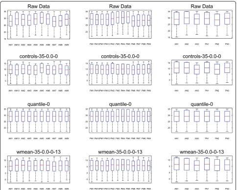
The proposed weighted mean normalization method could not be compared to quantile normalization in the same fashion as the other methods because quantile
normalization does not have a value analogous to CT0 which could be evaluated for stability and compared to weighted mean normalization. However, the normalized data resulting from each method could be visualized and compared as boxplots. Figure 8 shows the distributions of the raw and normalized data. All normalization meth-ods tend to decrease the variability compared to the raw data. Although quantile normalization forces all samples
Figure 7Comparison of theCT0values generated by different normalization methods. TheCT0calculations of each normalization method for each sample are shown here. The legend indicates the method used. The last number on the legend shows either thekvalue in a top-k calculation for the mean normalizations or the weighted mean power for the weighted mean normalizations.
Table 1 Mean Normalization
top-k meanCT0 stdev geNorm
1 20.92 0.69 0.35
2 23.2 0.64 0.21
3 23.8 0.64 0.19
4 22.13 0.63 0.2
5 22.11 0.61 0.17
6 22.79 0.6 0.18
7 22.91 0.61 0.16
8 23.66 0.59 0.15
9 23.67 0.6 0.16
10 23.61 0.61 0.16
∞ 25.59 0.71 0.23
MeanCT0calculations, standard deviations, and geNorm stability values for
using the mean of the top-k miRNAs with lowest standard deviation as the CT0value. An infinite value for k signifies the mean of all miRNAs. The best
values are marked in bold.
Table 2 Weighted Mean Normalization
power meanCT0 stdev geNorm
1 25.34 0.69 0.21
3 24.82 0.67 0.18
5 24.35 0.65 0.15
7 23.96 0.64 0.14
9 23.65 0.63 0.13
11 23.41 0.62 0.12
13 23.21 0.62 0.12
15 23.04 0.62 0.12
17 22.89 0.61 0.12
19 22.76 0.61 0.13
MeanCT0calculations, standard deviations, and geNorm stability values for
to have the same medians and distributions, Figure 8 shows that weighted mean normalization compares favorably with quantile normalization. Although the sam-ple medians and samsam-ple standard deviations resulting from weighted mean normalization differ slightly, they are generally uniform, and they are clearly more uniform than the endogenous control normalization. Weighted mean normalization also tends to have lower standard deviation than quantile normalization. For three samples in the second group (PM3, PM4, and PM5) that have higher expression in the raw data, weighted mean nor-malization results in medians and standard deviations which are similar to the other samples, while quantile normalization seems to produce greater standard devia-tion for these samples.
Table 3 Using the top 10 miRNAs as endogenous controls
miRNA meanCT0 stdev geNorm
191 20.92 0.69 1.14
744 25.49 0.72 1.17
152 25 0.73 1.12
MammU6 17.12 0.75 1.22
92a 22.03 0.75 1.24
29c 26.15 0.78 1.26
186 23.69 0.78 1.17
671-3p 28.89 0.8 1.29
26b 23.75 0.8 1.19
let-7d 23.07 0.8 1.16
MeanCT0calculations, standard deviations, and geNorm stability values
resulting from using each of the 10 miRNAs with lowest standard deviation.
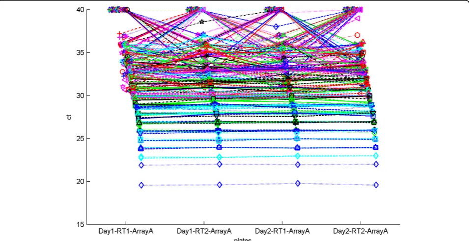
Having explored the problems of RT-PCR normaliza-tion, the consistency of miRNA expression experiments between RT-PCR and microarray technologies was of further interest to us. In order to explore this issue we used a dataset from Chen et al. [26], to explore the repro-ducibility of miRNA expression experiments across dif-ferent platforms. Chen et al. explored the effect of different reverse transcription reactions as well as the effect of pre-amplification of a sample. They concluded that different reverse transcription reactions did not result in significant variation in CT values. Because the samples in their dataset were highly consistent, as shown in Figure 9, this dataset was not suitable for the evalua-tion of the different normalizaevalua-tion methods presented in this work. We instead examined the effect of initial con-centration of a miRNA on its correlation with the micro-array experiment. Figure 10 contains a plot of theΔCT value vs. the base 2 logarithm of the microarray expres-sion for each miRNA for both cards in the experiment. The microarray data was log-transformed so that it would be on the same scale as the ΔCT values. We expect theΔCT values to correlate negatively with the microarray values since lowerΔCT values indicate higher expression, and Figure 10 shows that generally lower
ΔCT values are associated with higher microarray expression.
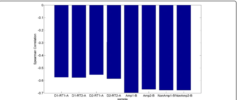
Figure 11 displays the Spearman correlation of each of the RT-PCR samples with the microarray data. The
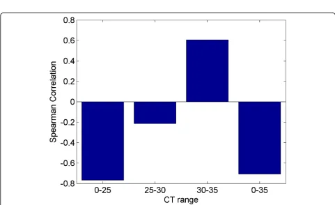
experiment used two different arrays or cards for RT-PCR. The card“A”contains well-characterized miRNAs, while card“B”contains newly discovered, less well-known miR-NAs [26]. We observe that card B is more highly corre-lated than card A. However, card A had 134 miRNAs detected that were also present on the microarray while card B only detected 29 miRNAs that were present on the microarray. Although the values are similar, the pre-ampli-fied samples have a higher correlation with the microarray than the non-amplified samples. Due to the bias described previously we expected to observe miRNAs with higher initial concentrations (lower CT values) to correlate better with the microarray. In order to test this hypothesis we partitioned the data from each card into bins based on CT ranges. In card “A”, contrary to our expectation, we observe that the Spearman correlation improves slightly for higher CT values as shown in Figure 12. We also observe that using all miRNAs results in a stronger corre-lation than any individual range of CT values. In Card“B,” shown in Figure 13, we do observe stronger correlation values with lower CT ranges. The highest bin, containing miRNAs with average CT values ranging from 30 to 35 contradicts the expectation of negative correlation, and we observe a large positive correlation, however this correla-tion is not significant, indicating that the measurement of the expression of the specific miRNAs that fell in this range exhibited considerable variability between RT-PCR and microarray data.
Conclusions
We explored the phenomenon whereby differences in the initial sample size of miRNA in an RT-PCR experiment were magnified with increasing CT levels. This was illu-strated by the strong correlation of the CT values of the individual miRNAs with the average CT values of all miR-NAs and by the increased sensitivity in the CT values of the low-abundant miRNAs to the average CT values. We conclude that a systematic bias in RT-PCR exists in which the fluctuations in the CT are dependent on the
expression levels of the particular miRNAs. We further proposed a novel data-driven method of addressing this bias by using the weighted mean instead of an endogenous control in the calculation ofΔCT. We demonstrated that the new normalization method produces lower standard deviations and is more stable than other methods.
Note that, while the power parameter in the weighted mean normalization method provides a convenient way of adjusting how much one wishes to let the less stable micro-RNAs influence the normalization of other micromicro-RNAs, its
Figure 10RT-PCR expression vs. log microarray expression. On the left each point represents the base 2 logarithm of the microarray expression vs. theΔCT value for a particular miRNA for card A. On the right is the same plot for card B.
Figure 12Correlation of card A by range of CT values. Here we divided the miRNAs detected on both card A and the microarray into ranges of CT values and calculated the Spearman correlation of the miRNAs’ΔCT values with the base 2 logarithm of their microarray expression.
optimization currently requires enumeration of different values and using the one with the best overall stability. Several CT0values can be calculated for different values for the weighted mean power, subsequently the value of the power that produces the lowest standard deviation or is determined to be the most stable by geNorm can be used for normalization. The standard deviation or geNorm stability calculations are two methods to quantitatively determine the ideal weighted mean power. Other criteria, such as significance of the differentially expressed micro-RNAs can be utilized in this optimization. Furthermore, a different customCT0value for each microRNA may be used, such that each microRNA is normalized differently, dependent on its average expression level.
We further examined the reproducibility of miRNA expression experiments across two different platforms by comparing RT-PCR and microarray results. We explored the relationship between the CT value and the consistency of the expression of a miRNA between RT-PCR and microarray. We leave as a future work the comparison of the ability of different normalization methods to detect differentially expressed genes.
Authors’contributions
AS conceived of the study and coordinated the project. RQ implemented the method and performed the experiments. RQ contributed to the design and testing of the method. All authors participated in the analysis of the results. RQ and AS contributed to the writing of the manuscript. All authors read and approved of the final draft.
Competing interests
The authors declare that they have no competing interests.
Published: 23 January 2013
References
1. Jukic D, Rao U, Kelly L, Skaf J, Drogowski L, Kirkwood J, Panelli M:Microrna profiling analysis of differences between the melanoma of young adults and older adults.Journal of Translational Medicine2010,8(1):27. 2. Schmeier S, Schaefer U, MacPherson CR, Bajic VB:dPORE-miRNA:
Polymorphic Regulation of MicroRNA Genes.PLoS ONE2011,6(2):e16657. 3. Han Y, Chen J, Zhao X, Liang C, Wang Y, Sun L, Jiang Z, Zhang Z, Yang R,
Chen J,et al:MicroRNA Expression Signatures of Bladder Cancer Revealed by Deep Sequencing.PLoS ONE2011,6(3):e18286.
4. Lee RC, Feinbaum RL, Ambros V:The C. elegans heterochronic gene lin-4 encodes small RNAs with antisense complementarity to lin-14.Cell1993,
75(5):843-854.
5. Lee RC, Ambros V:An Extensive Class of Small RNAs in Caenorhabditis elegans.Science2001,294(5543):862-864.
6. Bartel DP:MicroRNAs: Genomics, Biogenesis, Mechanism, and Function.
Cell2004,116(2):281-297.
7. Griffiths-Jones S, Grocock RJ, van Dongen S, Bateman A, Enright AJ:
miRBase: microRNA sequences, targets and gene nomenclature.Nucleic Acids Research2006,34(suppl 1):D140-D144.
8. Wang B, Wang X-F, Howell P, Qian X, Huang K, Riker AI, Ju J, Xi Y:A personalized microRNA microarray normalization method using a logistic regression model.Bioinformatics2010,26(2):228-234. 9. Rao Y, Lee Y, Jarjoura D, Ruppert Amy S, Liu C-g, Hsu Jason C, Hagan
John P:A Comparison of Normalization Techniques for MicroRNA Microarray Data.Statistical Applications in Genetics and Molecular Biology
2008,7.
10. Etheridge A, Lee I, Hood L, Galas D, Wang K:Extracellular microRNA: A new source of biomarkers.Mutation Research/Fundamental and Molecular Mechanisms of Mutagenesis2011,717(1-2):85-90.
11. Ambros V:The functions of animal microRNAs.Nature2004,
431(7006):350-355.
12. Friedman RC, Farh KK-H, Burge CB, Bartel DP:Most mammalian mRNAs are conserved targets of microRNAs.Genome Research2009,19(1):92-105. 13. Liang Y, Ridzon D, Wong L, Chen C:Characterization of microRNA
expression profiles in normal human tissues.BMC Genomics2007,
8(1):166.
14. Kim Y-K, Kim VN:Processing of intronic microRNAs.EMBO J2007,
26(3):775-783.
15. Mestdagh P, Van Vlierberghe P, De Weer A, Muth D, Westermann F, Speleman F, Vandesompele J:A novel and universal method for microRNA RT-qPCR data normalization.Genome Biology2009,10(6):R64. 16. Latham G:MicroRNAs and the immune system normalization of
MicroRNA quantitative RT-PCR data in reduced scale experimental designs.InMicroRNAs and the immune system..1 edition. Humana Press; Monticelli S 2010:19-31.
17. Gee HE, Buffa FM, Camps C, Ramachandran A, Leek R, Taylor M, Patil M, Sheldon H, Betts G, Homer J,et al:The small-nucleolar RNAs commonly used for microRNA normalisation correlate with tumour pathology and prognosis.Br J Cancer2011,104(7):1168-1177.
18. Croce CM:Causes and consequences of microRNA dysregulation in cancer.Nat Rev Genet2009,10(10):704-714.
19. Wang X:A PCR-based platform for microRNA expression profiling studies.RNA2009,15(4):716-723.
20. Livak KJ, Schmittgen TD:Analysis of Relative Gene Expression Data Using Real-Time Quantitative PCR and the 2-ΔΔCT Method.Methods2001,
25(4):402-408.
21. Bolstad BM, Irizarry RA, Åstrand M, Speed TP:A comparison of normalization methods for high density oligonucleotide array data based on variance and bias.Bioinformatics2003,19(2):185-193. 22. Irizarry RA, Hobbs B, Collin F, Beazer-Barclay YD, Antonellis KJ, Scherf U,
Speed TP:Exploration, normalization, and summaries of high density oligonucleotide array probe level data.Biostatistics2003,4(2):249-264. 23. Deo A, Carlsson J, Lindlof A:How to choose a normalization strategy for
miRNA quantitative real-time (QPCR) arrays.Journal of Bioinformatics and Computational Biology2011,09(06):795-812.
24. Mar J, Kimura Y, Schroder K, Irvine K, Hayashizaki Y, Suzuki H, Hume D, Quackenbush J:Data-driven normalization strategies for high-throughput quantitative RT-PCR.BMC Bioinformatics2009,10(1):110.
25. Edgar R, Domrachev M, Lash AE:Gene Expression Omnibus: NCBI gene expression and hybridization array data repository.Nucleic Acids Research
2002,30(1):207-210.
26. Chen Y, Gelfond J, McManus L, Shireman P:Reproducibility of quantitative RT-PCR array in miRNA expression profiling and comparison with microarray analysis.BMC Genomics2009,10(1):407.
27. Vandesompele J, De Preter K, Pattyn F, Poppe B, Van Roy N, De Paepe A, Speleman F:Accurate normalization of real-time quantitative RT-PCR data by geometric averaging of multiple internal control genes.Genome Biology2002,3(7):1-11.
doi:10.1186/1755-8794-6-S1-S14
Cite this article as:Qureshi and Sacan:A novel method for the normalization of microRNA RT-PCR data.BMC Medical Genomics2013