www.geosci-model-dev.net/9/2167/2016/ doi:10.5194/gmd-9-2167-2016
© Author(s) 2016. CC Attribution 3.0 License.
Determining lake surface water temperatures worldwide using a
tuned one-dimensional lake model (
FLake
, v1)
Aisling Layden1,a, Stuart N. MacCallum2, and Christopher J. Merchant3 14 Rose Hill, Sligo, Ireland
2School of Geosciences, University of Edinburgh, Grant Institute, The King’s Buildings, West Mains Road, Edinburgh,
EH9 3FE, UK
3Dept. of Meteorology, University of Reading, Harry Pitt Building, 3 Earley Gate, P.O. Box 238, Whiteknights, Reading,
RG6 6AL, UK
aformerly at: University of Edinburgh, School of Geosciences, Crew Building, Kings Buildings, West Main Rd, Edinburgh
EH9 3JN, UK
Correspondence to:Aisling Layden (aislinglayden99@gmail.com)
Received: 20 July 2015 – Published in Geosci. Model Dev. Discuss.: 8 October 2015 Revised: 4 May 2016 – Accepted: 6 May 2016 – Published: 15 June 2016
Abstract.A tuning method forFLake, a one-dimensional (1-D) freshwater lake model, is applied for the individual tuning of 244 globally distributed large lakes using observed lake surface water temperatures (LSWTs) derived from along-track scanning radiometers (ATSRs). The model, which was tuned using only three lake properties (lake depth, snow and ice albedo and light extinction coefficient), substantially im-proves the measured mean differences in various features of the LSWT annual cycle, including the LSWTs of saline and high altitude lakes, when compared to the observed LSWTs. Lakes whose lake-mean LSWT persists below 1◦C for part of the annual cycle are considered to be season-ally ice-covered. For trial seasonseason-ally ice-covered lakes (21 lakes), the daily mean and standard deviation (2σ )of abso-lute differences between the modelled and observed LSWTs are reduced from 3.07◦C±2.25◦C to 0.84◦C±0.51◦C by tuning the model. For all other trial lakes (14 non-ice-covered lakes), the improvement is from 3.55◦C±3.20◦C to 0.96◦C±0.63◦C. The post tuning results for the 35 trial lakes (21 seasonally ice-covered lakes and 14 non-ice-covered lakes) are highly representative of the post-tuning results of the 244 lakes.
For the 21 seasonally ice-covered lakes, the modelled re-sponse of the summer LSWTs to changes in snow and ice albedo is found to be statistically related to lake depth and latitude, which together explain 0.50 (Radj2 ,p=0.001) of the
inter-lake variance in summer LSWTs. Lake depth alone ex-plains 0.35 (p=0.003) of the variance.
Lake characteristic information (snow and ice albedo and light extinction coefficient) is not available for many lakes. The approach taken to tune the model, bypasses the need to acquire detailed lake characteristic values. Furthermore, the tuned values for lake depth, snow and ice albedo and light ex-tinction coefficient for the 244 lakes provide some guidance on improvingFLakeLSWT modelling.
1 Introduction
mesoscale weather processes causing lake-effect storms, al-tering the local climate (Sousounis and Fritsch, 1994; Long et al., 2007). Shallow lakes, particularly those with a large surface area, such as Lake Balaton, are more sensitive to at-mospheric events (Voros et al., 2010).
Reliable modelling of LSWTs can enrich our understand-ing of the highly variable dynamic nature of lakes. In this paper, a freshwater lake model, FLake (available at http: //www.flake.igb-berlin.de/sourcecodes.shtml), is tuned with along-track scanning radiometers (ATSR) Reprocessing for Climate: Lake Surface Water Temperature and Ice Cover (ARC-Lake) observations (MacCallum and Merchant, 2012) of 244 globally distributed lakes.FLakeis a one-dimensional (1-D) thermodynamic lake model, capable of predicting the vertical temperature structure and mixing conditions of a lake (Mironov et al., 2010). The tuned model is expected to im-prove the LSWT representation of these lakes inFLake.
There have been some studies carried out that compare modelled LSWTs from FLakewith LSWT observations on European lakes (Voros et al., 2010; Bernhardt et al., 2012; Pour et al., 2012). The findings from two of these three stud-ies showed consistent differences between the modelled and observed LSWTs (overestimation of the open water LSWTs and underestimation of the ice cover period). Despite these differences,FLake is considered to be a reliable model for simulating LSWTs and lake ice phenology (Bernhardt et al., 2012). The overestimation of the open water LSWTs and un-derestimation of the ice cover period are consistent with pre-liminary trial work findings from this study, which included North American and European lakes.
It is the intention of this study to achieve a daily mean ab-solute difference (MAD) of≤1◦C, between the tuned and
observed LSWTs, across all lakes. For each lake, the daily MAD quantifies the mean absolute difference in modelled and observed daily LSWT value, averaged over the total number of days. The dispersion of the daily MADs are re-ported to 2 standard deviations (±2σ )for each lake. When reported across a number of lakes, the daily MAD for each lake is averaged, with the dispersion of the MADs across in-dividual lakes reported to±2σ.
A daily MAD of ≤1◦C across all lakes, is possibly ac-curate enough for a global scale study. A lower daily MAD target may not be achievable as this study comprises of lakes with a wide range of geographical and physical characteris-tics. The effect of the tuning on the sub-surface temperature profile and on the depth of the mixed layer is not consid-ered in this study. Many lake-specific properties can be con-sidered inFLake. Preliminary model trial work was carried out on seven seasonally ice-covered lakes (deep and shal-low), which had available lake characteristic data in the ILEC world lake database (ILEC, 1999) or LakeNet’s Global Lake Database (LakeNet, 2003). Through this preliminary work, the lake-specific properties, which exerted the strongest ef-fect on the modelled LSWTs, were selected. These properties are lake depth (d), snow and ice albedo (α)and light
extinc-tion coefficient (κ). In the next part of the preliminary work, it was determined that the modelled LSWTs could be tuned to compare well with the observed LSWTs, by adjusting the values for these three properties:d,αandκ, herein referred to LSWT-regulating properties. On the basis of the prelimi-nary findings, the trial work was performed on 35 lakes, prior to attempting to tune all 246 lakes.
An example of the preliminary trial work is shown in Fig. 1a, for Lake Athabasca, Canada (mean depth of 26 m). In this figure, a greater modelledα(higher reflectivity) results in a later ice-off date than the default model snow and ice albedo and is closely comparable to the observed ice-off date. In Fig. 1b, it is demonstrated that by using a shallowerdthan the mean depth of the lake, the ice-on day occurs earlier and corresponds more closely to the observed ice-on day. Lake depth is essentially being used as a means to adjust the heat capacity of the lake, exerting control over the lake cooling and therefore the ice-on date. The modelled LSWT is further improved by lowering theκ value (greater transparency).
The greater transmission of surface heat to the lower layer results in a lower (and more representative) maximum LSWT, Fig. 1b. The LSWTs modelled using the greaterα, lower d and lower κ compare closely with the observed LSWTs, Fig. 1c.
In this study, the modelled mean differences for several features in the LSWT annual cycle are measured, quanti-fying the level of agreement with the observed ARC-Lake LSWTs, are the basis for selecting the tuned (optimal) LSWT-regulating properties (d,αandκ)for each lake. Lakes are divided into two distinct categories. Lakes with a lake-mean LSWT climatology (determined using twice-a-month ARC-Lake full-year LSWT observations, 1992/1996–2011) remaining below 1◦C for part of the seasonal cycle are
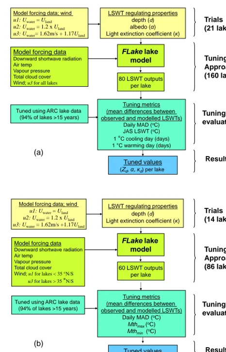
cate-gorised as seasonally ice-covered lakes (160 lakes). All other lakes are categorised to as non-ice-covered lakes (86 lakes). Although some of the seasonally ice-covered lakes may not be completely ice-covered during the cold season and some of the non-ice-covered lakes may have short periods of par-tial ice cover, the 1◦C lake-mean LSWT offers a good means of evaluating lakes that are typically and non-typically ice-covered during the coldest part of the LSWT cycle. To best capture the critical features of both seasonally ice-covered and non-ice-covered lakes, the mean difference in the fea-tures between the observed and modelled LSWTs differ with lake category. The tuning approach applied to these two lake categories is summarised in Fig. 2, and described in detail within Sect. 2.3.
glob-Figure 1.Preliminary modelled runs for Lake Athabasca, Canada
(59◦N 110◦W), showing that adjustments to lake depth (d), snow
and ice albedo (α)and light extinction coefficient (κ)can greatly
improve the modelled lake surface water temperatures (LSWTs)
compared to the default/recommendedd,αandκvalues;(a)shows
that a higherαcauses a later ice-off date, comparing well with the
observed (ARC-Lake) ice-off date,(b)shows that a lowerdcauses
an earlier ice-on date and a lowerκvalue (greater transparency)
re-duces the maximum LSWT and(c)shows that the combined effect
of the adjustedd,αandκproduce LSWTs that are highly
compa-rable to the observed ARC-Lake LSWTs.
ally, offering the potential to help develop parameterisation schemes for lakes in numerical weather prediction models. It is expected that the findings in this study will be of interest to climate modellers, limnologists and current and perspective users ofFLake.
2 Methods
2.1 Data: ARC-Lake observed LSWTs
LSWT observations from ARC-Lake are used to tune the model. These cover 246 globally distributed large lakes, principally those with surface area>500 km2(Herdendorf, 1982; Lehner and Döll, 2004) but also including 28 globally distributed smaller lakes, the smallest of which is 100 km2
Model forcing data Downward shortwave radiation Air temp
Vapour pressure Total cloud cover Wind; u3 for all lakes
FLake lake model
LSWT regulating properties depth (d) albedo (α) Light extinction coefficient (κ)
80 LSWT outputs per lake
Tuned using ARC lake data (94% of lakes >15 years)
Tuning metrics (mean differences between observed and modelled LSWTs)
Daily MAD (oC) JAS LSWT (oC) 1 °C cooling day (days) 1 °C warming day (days)
Tuned values
(Zd, α, κd) per lake
Trials (21 lakes)
Tuning Approach (160 lakes)
Model forcing data; wind u1: Uwater = Uland
u2: Uwater = 1.2 x Uland
u3: Uwater= 1.62m/s + 1.17Uland
Result Tuning evaluation
(a)
FLake lake model
60 LSWT outputs per lake
Tuned using ARC lake data (94% of lakes >15 years)
Tuning metrics (mean differences between observed and modelled LSWTs)
Daily MAD (oC)
Mthmax (oC)
Mthmin (oC) Tuned values
(Zd, κd) per lake
Trials (14 lakes)
Tuning Approach (86 lakes)
Model forcing data; wind u1: Uwater = Uland
u2: Uwater = 1.2 x Uland
u3: Uwater = 1.62m/s +1.17Uland
Result Tuning evaluation
(b)
LSWT regulating properties depth (d)
Light extinction coefficient (κ)
Model forcing data Downward shortwave radiation Air temp
Vapour pressure Total cloud cover Wind; u1 for lakes < 35 °N/S
u3 for lakes > 35 °N/S
Figure 2.Study approach overview (trials, tuning, evaluation and
results) for(a)seasonally ice-covered lakes and(b)non-ice-covered
lakes. For the trials, wind speed scaling,u1,u2 (recommended for
lakes with fetch>16 km) andu3 (recommended for open ocean
water) is assessed on the untuned model, tuning is then trialled
with a range of factors fordand values forαandκusing the
se-lected wind speed scaling. The tuning approach produces modelled
LSWTs for all possible combination ofd,αand κ, 80 modelled
runs for seasonally ice-covered lakes and 60 for non-ice-covered lakes. For the evaluation, the tuning metrics (normalised and equally weighted) are the basis for selection of the optimal (tuned) LSWT model for each lake.
(Lake Vesijarvi, Finland). The LSWTs are generated from three ATSRs, from August 1991–December 2011 (MacCal-lum and Merchant, 2012).
analy-Figure 3.Location of 246 observed lakes colour coded by surface area (obtained using polygon area in Global Lakes and Wetlands Database (GLWD) showing zoomed inset of North America and northern Europe.
sis of the average (over the period of ATSR observations) days of the year on which the lake-mean LSWT drops be-low 1◦C and rises above 1◦C. Layden et al. (2015) defined these as the 1◦C cooling and 1◦C warming days respectively, and observe good consistency with in situ measurements of ice-on and ice-off days for 21 Eurasian and North American lakes. Layden et al. (2015) also demonstrated the integrity of the ARC-Lake LSWTs on a global scale, through the strong relationship the observed LSWTs have with meteorological data (air temperature and solar radiation) and geographical features (latitude and altitude).
An average of the day and night lake-mean LSWT obser-vations from 8 August 1991 to the end of 2010 is used to tune the model. The final year of observations (2011) is retained to carry out an independent evaluation on the tuned model. For 119 lakes, there are continuous LSWT observations for 20 years (all three ATSR instruments, from August 1991 to December 2011), 113 lakes have 16 years of continuous LSWT observations (2 ATSR instruments) and 14 lakes have 8–9 years of LSWT observations (1 ATSR instrument). The location of the 246 lakes (55◦S to 69◦N), classified by sur-face area, using polygon area in Global Lakes and Wetlands Database (GLWD; Lehner and Döll, 2004) is shown in Fig. 3.
2.2 Model:FLakelake model
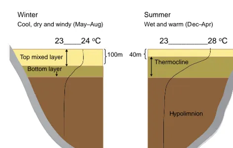
FLakeis a two-layer parametric representation of the
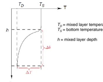
evolv-ing temperature profile of a lake and is based on the net en-ergy budgets (Mironov, 2008). The depth and temperature of the homogeneous “upper mixed layer” and the temperature of the “lake bottom” (representative of the hypolimnion tem-perature), as illustrated in Fig. 4, are modelled inFLake. The thermal structure of the intermediate stratified layer (ther-mocline, Fig. 4) is parameterised in FLake through a self-similarity representation of the temperature profile,υ(ζ ), us-ing time (T) and depth (z) as illustrated in Fig. 5.
23____24 oC 23_________28 oC
Top mixed layer
Bottom layer
Winter Summer
Cool, dry and windy (May– ug) Wet and warm ( D ec– Apr)
Thermocline
H ypolimnion
100m 40m
Figure 4. Winter and summer depth and temperature profile for
Lake Malawi (mean depth of 273 m), Africa (12◦S 35◦E),
illus-trated using data from the ILEC world lake database (http://wldb. ilec.or.jp/), showing the three distinct layers (in winter and summer)
of a deep stratified non-ice-covered lake.FLake, a two-layer model,
predicts the depth and temperature of the “upper mixed layer” and the temperature of the “bottom layer” (shown on the left), and “ther-mocline” depth and temperature profile (shown on the right).
FLake utilises the minimum set of input data required
for 1-D thermal and ice models: meteorological forcing data (shortwave and long-wave radiation, wind speed, air vapour pressure and air temperature), an estimation of turbidity and basic bathymetric data (Lerman et al., 1995). Although mod-els based on the concept of self-similarity are considered to be only fairly accurate (Dutra et al., 2010), we show that mean differences between the model and observed LSWTs are greatly lowered by tuning the model.
2.2.1 Lake-specific model properties
(α)and light extinction coefficient (κ))can greatly improve the LSWTs simulated inFLake. Other lake-specific proper-ties adjusted for this study are c_relax_C, fetch, latitude and the starting conditions.
c_relax_C: a dimensionless constant used in the relaxation equation for the shape factor with respect to the temperature profile in the thermocline.
The default value of 0.003 was found to be too low to adequately readjust the temperature profile of deep lakes (G. Kirillin, personal communication, 2010), weakening the predicted stratification and affecting the LSWT. For lakes with mean depths<5 m, the c_relax_C value is set to 10−2, and decreases with increasing depth, to a value of 10−5for mean depths >50 m, as recommended by G. Kirillin (per-sonal communication, 2010).
Fetch: wind fetch is calculated as the square root of the product of lake length and breadth for the 205 (of 246) lakes with available dimensions. A line fit on the calculated fetch versus polygon area (in units of km and km2 respectively) from the GLWD (Lehner and Döll, 2004) of these 205 lakes, showed a strong relationship between fetch and area, Eq. (1), Radj2 =0.84,p=0.001. Equation (1), used to determine the fetch of the remaining 41 lakes with no available dimensions, is valid for lakes>100 km2. Although the shape of a lake and its orientation in relation to wind direction are likely to affect wind fetch, this approach is expected to provide reasonable estimates of fetch.
fetch=39.9 km+0.00781×area×km−1 (1) Latitude: the latitude of the lake centre reference co-ordinates (Herdendorf, 1982; Lehner and Döll, 2004).
Starting conditions: provide the initial lake-specific upper mixed layer temperature and depth, bottom temperature, ice thickness and air–ice interface temperature, were shown to shorten the model spin-up time (to an average of<3 days). A good estimation of the starting conditions was obtained from
the FLake model based on the hydrological year 2005/06
(Kirillin et al., 2011).
2.2.2 Fixed model parameters
The icewater_flux, inflow from the catchment and heat flux from sediments remain fixed throughout the investigative and tuning process, across all lakes. For icewater_flux, (heat flow from water to ice) G. Kirillin (personal communication, 2010) suggested values of∼3–5 W m−2. In this study a value of 5 W m−2is applied to all lakes. Inflow from the catchment
and heat flux from sediments are not considered. 2.2.3 Model forcing data
FLake is forced with ECMWF Interim Re-analysis (ERA)
data (Dee et al., 2011; ECMWF, 2009), at the grid points (0.7◦×0.7◦resolution) closest to the lake centre, shown in the Supplement. The mean daily values of shortwave
so-Figure 5 Schematic representation of the temperature profile in the upper mixed layer and in the thermocline, reproduced from Killirin (2003). The self-similarity representation of the temperature profile in FLake is determined using dimensionless co-ordinates, ζ = ( z-h)/Δh, and υ = [T(z)-TD]/ΔT.
TD = mixed layer temperature
TS = bottom temperature
h = mixed layer depth
Figure 5.Schematic representation of the temperature profile in the upper mixed layer and in the thermocline, reproduced from Kil-lirin (2003). The self-similarity representation of the temperature
profile inFLakeis determined using dimensionless co-ordinates,
ζ=(z−h)/1handυ= [T (z)−TD]/1T.
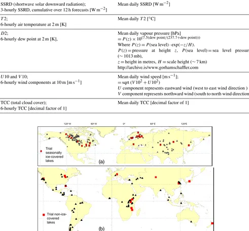
lar downward radiation (SSRD), air temperature and vapour pressure at 2 m, wind speed at 10 m and total cloud cover (TCC), shown in Table 1, are used to force the model. 2.3 Tuning method
A range of factors/values for d, α and κ is determined through the model trials (carried out on 21 seasonally ice-covered lakes and 14 non-ice-ice-covered lakes, Fig. 6). These lakes broadly represent the range of lake characteristics – lake depth, snow and ice albedo and light extinction coef-ficient – and have available Secchi disk depth data.
2.3.1 Light extinction coefficients for trial lakes
The light extinction coefficient values for the untuned model trial are derived from Secchi disk depth data,κsd(in units of
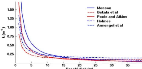
m−1), obtained from the ILEC database (ILEC, 1999). Five methods of relating κ values to Secchi disk depths (Poole and Atkins, 1929; Holmes, 1970; Bukata et al., 1988; Mon-son, 1992; Armengol et al., 2003) are compared in Fig. 7. These methods cover a range of different water conditions, from coastal turbid waters (Holmes, 1970) and eutrophic wa-ter (tested 1 km from a dam in the Sau reservoir, Spain) (Ar-mengol et al., 2003) to a range of North American lakes of different trophic levels (Monson, 1992).
For Secchi disk depths>10 m, all methods show a rea-sonably good comparison between Secchi disk depths andκ, Fig. 7. From Secchi disk depths of 10 to 1 m, the range of re-sults between methods becomes increasingly large. Bukata et al. (1998) showed that Eq. (2), based on in situ opti-cal measurements from many stations, adequately described Lake Huron, Lake Superior and Lake Ontario, for Secchi disk depths from 2 to 10 m:
κsd=(0.757/S)+0.07 m−1 (2)
Table 1.ECMWF Interim Re-analysis (ERA) data components andFLakeinput format. Units are given in square brackets.
ERA data components and description FLakeinput
SSRD (shortwave solar downward radiation);
3-hourly SSRD, cumulative over 12 h forecasts [W m−2]
Mean daily SSRD [W m−2]
T2;
6-hourly air temperature at 2 m [K]
Mean dailyT2 [◦C]
D2;
6-hourly dew point at 2 m [K],
Mean daily vapour pressure [hPa]
=P (z)×10(7.5(dew point/(237.7+dew point)))
WhereP (z)=P(sea level)·exp(−z/H ).
P (z)=pressure at height z, P(sea level)=sea level pressure
(∼1013 mb),
z=height in metres,H=scale height (∼7 km)
http://archive.is/www.gorhamschaffler.com
U10 andV10;
6-hourly wind components at 10 m [m s−1]
Mean daily wind speed [m s−1];
=sqrt (V102+U102)
Ucomponent represents eastward wind (west to east wind direction )
Vcomponent represents northward wind (south to north wind direction)
TCC (total cloud cover);
6-hourly TCC [decimal factor of 1]
Mean daily TCC [decimal factor of 1]
b) a)
Figure 6 Location of lakes, with red square showing the trial lakes a) 160 seasonally ice-covered lakes, including 21 trial lakes and b) 86 non-ice covered lakes including 14 trial lakes
120o W 60o W 0o 60o E 120oE
( a)
( b)
Trial seasonally ice-covered lakes
Trial non-ice- covered lakes
Figure 6.Location of lakes, with red square showing the trial lakes(a)160 seasonally ice-covered lakes, including 21 trial lakes and(b)86 non-ice-covered lakes including 14 trial lakes.
Equation (2), applied in this study for lakes with Secchi disk depths of 2–10 m, produces the lowest (most transpar-ent)κ values, potentially more representative of open water conditions of large lakes. For lakes outside this Secchi disk depth range (less than 2 m and greater than 10 m), the Poole and Atkins (1929) formula, Eq. (3), is applied, providing suf-ficiently accurate estimations of light extinction coefficients in waters with all degrees of turbidity (Sherwood, 1974).
κsd=1.7/S (3)
2.3.2 Light extinction coefficients for tuning of all lakes
Figure 7.A comparison of five methods relating light extinction co-efficients to Secchi disk depths, showing that all methods compare
reasonably well at Secchi disk depths>10 m.
all lakes. A range of 10 optical water types, which essen-tially describe the attenuation process of ocean water and its changes with turbidity (Jerlov, 1976), is applied. These con-sist of five optical water types for open ocean, type I, IA, IB, II and III; type I being the most transparent and type III be-ing least transparent and five coastal ocean types (1, 3, 5, 7 and 9) (Jerlov, 1976). The spectrum for these 10 ocean water types are divided (in fractions of 0.18, 0.54, 0.28) into bands represented by three wavelengths: 375, 475 and 700 nm re-spectively. The 10 ocean water types are renamed herein as κd1toκd10, the values for which are shown in Table 2. 2.3.3 Tuning of lake depth
Lake depth information was obtained from Herden-dorf (1982), the ILEC World Lake Database (http:// wldb.ilec.or.jp/), LakeNet (http://www.worldlakes.org/) and Kourzeneva et al. (2012). The mean depth (Zd1)is the
rec-ommended depth value for FLake. Where only maximum depth is available (nine lakes), the mean depth is calculated using the average maximum-to-mean depth ratio of lakes with known maximum and mean depths. This ratio is 3.5 for seasonally ice-covered lakes and 3.0 for non-ice-covered lakes. In the tuning process, depth factors (outlined in Ta-ble 2) are applied to the lake-mean depth. The tuned depth is referred to as the “effective depth”. For lakes with no depth information, the effective depth factors are applied to a depth of 5 m. If the resulting effective depth is too shallow, charac-terised by early LSWT cooling and/or a high summertime LSWTs: July–August–September (JAS) LSWTs, tuning is repeated using a deeper input depth.
For modelling very deep lakes, a “false depth” is recom-mended (G. Kirillin, personal communication, 2010). For the six lakes with mean depths in excess of 240 m (ranging from 240 m for Lake Kivu to 680 m for Lake Baikal), false depths of 100–200 m are used in the tuning study.
2.3.4 Tuning of snow and ice albedo
FLake uses two categories of albedo for snow (dry snow
and melting snow) and for ice (white ice and blue ice). As the snow cover module is not operational in this version of
FLake, the snow and ice albedo are set to the same default
value in the albedo module; 0.60 for dry snow and white ice and 0.10 for melting snow and blue ice. An empirical for-mulation is applied inFLake, where the albedo of a frozen lake surface (αlake)depends on the ice surface temperature
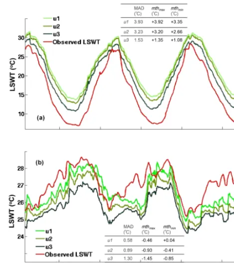
(Eq. 4) (Rooney and Jones, 2010), accounting somewhat for seasonal changes in albedo (Mironov and Ritter, 2004). By application of this equation, the blue ice (by means of its albedo) has greater influence on the rate of ice melting, in the warming season.
αlake=αw+(αb−αw)exp[−Cα(T0−Tp)/T0], (4)
where αw=white ice albedo (0.60), αb=blue ice albedo
(0.10), Cα=Ice albedo empirical coefficient (95.6), T0=freezing temperature (K) and Tp=the surface tem-perature (K) from the previous time step. The extinction coefficient values used for modelling solar radiation penetra-tion through white ice and blue ice are 17.1 and 8.4 (in units of m−1)respectively, and correspond to the top 0.1 m of the ice layer for clear-sky conditions (Launiainen and Cheng, 1998).
The default snow and ice albedo values are referred to as α1 in this study. During the preliminary trials, a higher albedo (thanα1) was shown to delay ice-off, substantially improving the timing of early ice-off, compared to observed LSWTs (demonstrated in Fig. 1a). A higher snow and ice albedo causes more of the incoming radiation to be reflected, resulting in a later ice-off. On this basis, we apply three ad-ditional higher albedo values (α2 :α4), shown in Table 2, for tuning seasonally ice-covered lakes. Albedo when discussed throughout this study refers to the albedo of snow and ice. The albedo of water (in liquid phase) is maintained at the default value of 0.07 throughout this study.
2.3.5 Wind speed scaling
Scaling of wind speeds is considered during the trials, as most long-term records of wind speed are measured over land (Uland)and are considered to underestimate the wind
speed over water (Uwater). For adjusting surface wind speeds
Table 2.Effective depth factors (Zd), light extinction coefficient values (κd)and snow and ice albedo values (α)used in tuning study;
80 possible combinations used for tuning of seasonally ice-covered lakes (Zd1:Zd4×κd1:κd5×α1 :α4). The modified tuning for the 25
shallow seasonally ice-covered lakes utilised greater depth factors;Zd6:Zd8and two higher light extinction coefficient values,κd6andκd7;
60 possible combinations used for tuning of non-ice-covered lakes (Zd1:Zd6×κd1:κd10). The spectre for the 10κdvalues are divided (in
fractions of 0.18, 0.54, 0.28) into bands represented by three wavelengths: 375, 475 and 700 nm respectively.
Effective depth Light extinction coefficient Albedo Snow and Melting
factors (κd) (α) white ice snow and blue
(Zd) Albedo ice albedo
κd 375 nm 475 nm 700 nm
Zd1 κd1 0.038 0.018 0.56 α1 0.60 0.10
κd2 0.052 0.025 0.57 α2 0.80 0.60
Zd2(Zd1·0.75) κd3 0.066 0.033 0.58 α3 0.80 0.40
Zd3(Zd1·0.5) κd4 0.122 0.062 0.61 α4 0.60 0.30
Zd4(Zd1·1.5) κd5 0.22 0.116 0.66
κd6 0.80 0.17 0.65
Zd5(Zd1·0.3) κd7 1.10 0.29 0.71 Zd6(Zd1·2.5) κd8 1.60 0.43 0.80 Zd7(Zd1·2.0) κd9 2.10 0.71 0.92 Zd8(Zd1·4.0) κd10 3.00 1.23 1.10
speed scalings are determined.
Uwater=1.62 m s−1+1.17Uland, (5)
where Uwater=wind speed over water and Uland=surface
wind speed over land
2.3.6 Summary of the tuning of the LSWT-regulating properties
Table 2 contains a summary of the factors/values for d, α andκ applied in this tuning study. The model is tuned using the optimal combination of LSWT-regulating properties; 80 possible combinations for seasonally ice-covered lakes and 60 possible combinations for non-ice-covered lakes. 2.4 Tuning metrics
The tuning metrics are the mean differences (between the modelled and the observed LSWTs), used to quantify the effect that the LSWT-regulating properties have on the modelled LSWTs. The metrics (normalised and equally weighted) determine the optimal LSWT model selected for each lake.
2.4.1 Tuning metrics for seasonally ice-covered lakes
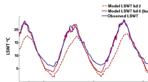
The metrics and the effect of the LSWT-regulating proper-ties on them, for seasonally ice-covered lakes is summarised in Table 3. The effect of light extinction coefficient on the JAS LSWTs is demonstrated in Fig. 8, showing that the tuned light extinction coefficient (κd)value,κd6in place of a lower
(more transparent)κdvalue (κd2), described in Table 2,
sub-stantially improves the JAS LSWTs. In this figure, the greater effect of light extinction coefficient on the maximum LSWT
Figure 8. Lake surface water temperatures (LSWTs) for Lake
Geneva, Europe (46◦N 6◦E), modelled with two differentκd
val-ues (κd2κd6; Table 2) shows the substantially stronger effect ofκd
on the maximum LSWT than the minimum LSWT.
than on the minimum LSWT is also demonstrated. The in-fluence of the effective depth over the 1◦C cooling day (the day the lake-mean LSWT drops below 1◦C; an indicator of ice-on) is demonstrated in Fig. 9. The 1◦C warming day (the day the lake-mean LSWT rises to above 1◦C; an indicator of ice-off) is strongly influenced by snow and ice albedo, as demonstrated in Fig. 1a.
2.4.2 Tuning metrics for non-ice-covered lakes
For these lakes, the daily MAD and the difference between the observations and model for the months, where the min-imum and maxmin-imum observed LSWTs occur (mthmin and
mthmax), are applied as metrics. Although there no
rec-Table 3.Relationship between the lake surface water temperature (LSWT)-regulating properties and metrics, showing the equations for determining the daily mean absolute difference (MAD) and the July–August–September (JAS) LSWT mean difference. Units are given in square brackets.
LSWT-regulating properties Effect on metric Metrics (mean differences between
ob-served and modelled LSWTs)
κ
(light extinction coefficient)
κaffects irradiance transmission of
sur-face water, which is more notable in summer months.
JAS LSWT mean difference
[◦C]=(ximod−jas−xobsi −jas)
mod−jas=modelled JAS LSWT
obs−jas=observed JAS LSWT
d
(depth)
d alters heat storage capacity affecting
timing of the start of the cold phase (the
day that the LSWT drops to below 1◦C)
1◦C cooling day
mean difference [days]
α
(snow and ice albedo)
α alters ice/snow reflectance affecting
the end of the cold phase (the day that
the LSWT increases to above 1◦C)
1◦C warming day
mean difference [days]
d,αandκ All LSWT-regulating properties
con-tribute to the comparability of the mod-elled and observed LSWT
Daily MAD [◦C]=P
(abs(ximod−
xiobs))/N;
mod=daily modelled LSWTs
obs=daily observed LSWTs
N=sample size
Figure 9. Effect of depth on the lake surface water temperature
(LSWT) for Lake Ladoga, Russia (61◦N 31◦E) (mean depth 52 m),
showing that when modelled at a greater depth, the lake cools later and the maximum LSWT is lower.
onciling the modelled monthly extremes with the observed monthly extremes.
2.4.3 Additional metrics for seasonally ice-covered lakes and non-ice-covered lakes
For each lake, the fraction of the observed mean LSWT vari-ance over the number of years with observations, accounted for in the tuned model is used to help independently evaluate the tuned LSWTs. For non-ice-covered lakes, the variance is determined using varmin(and varmax): the variance in the
mean LSWT for the month in which the minimum (and max-imum) LSWT is observed. For seasonally ice-covered lakes, the variance is determined using varjas: the variance in the
observed mean JAS LSWTs. The fraction of these observed
LSWT variances accounted for in the tuned model are quan-tified; intermin, intermaxand interjas(usingR2adj). The
calcu-lations to quantify varjasand interjasare shown in Eqs. (6) to
(8).
varjas: observed JAS LSWT variance (in units of K2)over
the length of the tuning period (Walker and Shostak, 2010): varjas=
X
(xiobs−jas−x)2/(N−1), (6) wherexobs−jas=observed mean JAS LSWTs for each indi-vidual yearx=mean across all years,N=number of years with JAS LSWTs interjas: the fraction of the observed JAS
LSWT inter-annual variance (varjas) accounted for in the
tuned model (Lane et al., 2016):
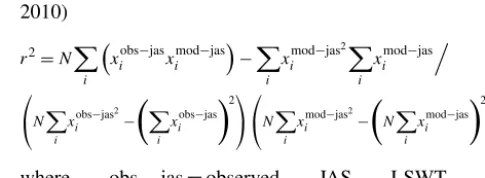
interjas=1−((1−r2)(N−1)/(N−P−1)), (7)
whereP=total number of regressors (Walker and Shostak, 2010)
r2=NX
i
xiobs−jasximod−jas−X i
xmodi −jas2X
i
ximod−jas. (8)
N X
i xobs−jas
2
i −
X
i xobsi −jas
!2
N X
i xmod−jas
2
i − N
X
i ximod−jas
!2
where obs−jas=observed JAS LSWT and mod−jas=modelled JAS LSWT.
The same equations, Eqs. (6) to (8), are applied to de-termine Intermax, varmax, intermin and varmin, substituting
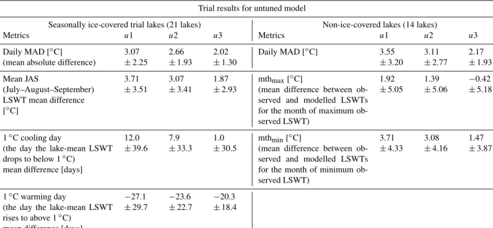
Table 4. The effect of wind speed scaling on untuned modelled LSWTs, presented as the mean difference, between the modelled and
observed values, across lakes with the spread of differences defined as 2σ, where wind speedsu1 is unscaled,u2 is factored by 1.2 andu3
(Uwater=1.62 m s−1+1.17Uland). Results are presented for seasonally ice-covered and non-ice-covered trial lakes. Results highlight that
u3 is most applicable to seasonally ice-covered lakes but there is no one wind speed most suited for all lakes (while the mean difference
is improved withu3, the spread of the mean differences across lakes for mthminand mthmaxshow little change). Units are given in square
brackets.
Trial results for untuned model
Seasonally ice-covered trial lakes (21 lakes) Non-ice-covered lakes (14 lakes)
Metrics u1 u2 u3 Metrics u1 u2 u3
Daily MAD [◦C]
(mean absolute difference)
3.07 ±2.25 2.66 ±1.93 2.02 ±1.30
Daily MAD [◦C] 3.55
±3.20 3.11 ±2.77 2.17 ±1.93 Mean JAS (July–August–September) LSWT mean difference [◦C]
3.71 ±3.51 3.07 ±3.41 1.87 ±2.93
mthmax[◦C]
(mean difference between ob-served and modelled LSWTs for the month of maximum ob-served LSWT) 1.92 ±5.05 1.39 ±5.06 −0.42 ±5.18
1◦C cooling day
(the day the lake-mean LSWT
drops to below 1◦C)
mean difference [days]
12.0 ±39.6 7.9 ±33.3 1.0 ±30.5
mthmin[◦C]
(mean difference between ob-served and modelled LSWTs for the month of minimum ob-served LSWT) 3.71 ±4.33 3.08 ±4.16 1.47 ±3.87
1◦C warming day
(the day the lake-mean LSWT
rises to above 1◦C)
mean difference [days]
−27.1 ±29.7 −23.6 ±22.7 −20.3 ±18.4
obs–max (and mod–max)=mean-observed LSWTs (and modelled LSWTs) in the month where the maximum LSWT occurs.
3 Trial results for wind speed scaling
For both seasonally ice-covered lakes and non-ice-covered lakes, wind speeds,u1,u2 andu3 were modelled with un-tuned LSWT properties: mean lake depth (Zd1), default snow
and ice albedo (α1) and light extinction coefficient derived from Secchi disk depth data (κsd). The trials show that wind
speed has a consistent effect on the modelled LSWT of seasonally ice-covered lakes. The higher wind speed scal-ing (u3) causes earlier coolscal-ing and later warmscal-ing (reduc-ing the 1◦C cooling day and 1◦C warming day mean dif-ferences), lengthening the ice cover period and lowering the JAS LSWT, as demonstrated for Lake Simcoe, Canada, in Fig. 10. It is expected that the tuning of d,α andκ, with an applied wind speed ofu3, will produce modelled LSWTs substantially closer to the observed LSWTs than those shown in Fig. 10, where tuning ofd,αandκ is not applied. The more rapid mixing and heat exchange between the surface and atmosphere, as a result of the higher wind speed, causes an earlier modelled 1◦C cooling day. As wind promotes ice growth in the model, higher wind speeds also contribute to the later-modelled 1◦C warming day. Wind speed scaling, u3 in place ofu1, for the trial seasonally ice-covered lakes,
reduces the mean difference in the length of the average cold phase (when compared to the observed cold phase) by
∼50 % (from 39 to 21 days) and reduces the JAS LSWT mean difference by∼50 %, from 3.71 to 1.87◦C, Table 4. For non-ice-covered trial lakes, five of the seven lakes at lat-itudes>35◦N/S (north or south) show best results withu3, as demonstrated for Lake Biwa, located at 35.6◦N, Fig. 11a. Five of the seven lakes located<35◦N/S show the best re-sults withu1, as demonstrated for Lake Turkana, located at 3.5◦N, Fig. 11b.
For the remainder of the tuning trials (tuned using the range ofd,αandκfactors/values outlined in Table 2), wind speed scalingu3 was applied to all seasonally ice-covered and to non-ice-covered lakes>35◦N/S and no scaling (u1) to non-ice-covered lakes<35◦N/S. As the daily MAD tar-get of<1.0◦C is met for both lake categories (shown in the
second results column in Table 5), the tuning approach de-scribed here is applied to all lakes.
4 Results
4.1 Summary of results
un-Figure 10.Effect of wind speed scalings on the modelled lake
sur-face water temperature (LSWT) for Lake Simcoe, Canada, 44◦N
79◦W (depth 25 m), showing that the greatest wind speed
scal-ing,u3 (Uwater=1.62 m s−1+1.17Uland), in place of the unscaled
wind speed, u1, reduces the daily mean absolute difference and
July–August–September LSWT mean difference by∼50 %.
Mod-elled with untuned LSWT properties: mean lake depth (Zd1),
de-fault snow and ice albedo (α1) and light extinction coefficient are
derived from Secchi disk depth data (κsd)
tuned model to 0.84◦C±0.51◦C and 0.96◦C±0.63◦C for the tuned model, Table 5. The tuned values for the LSWT-regulating properties for all lakes and the tuning metrics are shown in the Supplement.
These results demonstrate that the tuning process with the applied wind speed scalings can provide significant improve-ments on the untuned model: run using the lake mean depth, light extinction coefficients derived from Secchi disk depth (as shown in Sect. 2.3.1) and the model default albedo (sea-sonally ice-covered lakes only).
The applied tuning method yielded a daily MAD of 0.74◦C±0.48◦C, across 135 of the 160 seasonally covered lakes, Table 6. The remaining 25 seasonally ice-covered lakes yielded comparatively poor results; the 1◦C cooling day was 14 days too early and/or the JAS LSWT was
≥2◦C higher than observed LSWTs. Re-tuned using greater effective depth factors and higher κd values, as outlined in the next sub-section (Sect. 4.1.1), yielded a daily MAD of 1.11◦C±0.56◦C, across the 25 lakes. Across the 160 lakes, a daily MAD of below 1◦C was achieved (0.80◦C±0.56◦C, Table 5). A daily MAD of below 1◦C is again achieved (0.96◦C±0.66◦C) when 84 of the 86 non-ice-covered lakes are considered (Table 5). The remaining two lakes yielded highly unsatisfactory results.
4.1.1 Seasonally ice-covered lakes
The 25 lakes that were re-tuned are shallow (average mean depth<5 m) and small (18 of the 25 lakes are<800 km2), relative to the depth and area of the larger seasonally ice-covered lakes. Twenty (20) of the 25 lakes are located in eastern Europe or Asia, at relatively low altitudes; 22 of the 25 lakes are<752 m a.s.l. On initial tuning, these 25 lakes were tuned to the highest depth factor, Zd4 (1.5 times the
mean depth) and/or the highest light extinction coefficient,
Figure 11.Effect of wind speed scaling on lake surface water
tem-peratures (LSWTs) for a temperate non-ice-covered lake(a)Lake
Biwa, Japan (36◦N 136◦E), and for a tropical non-ice-covered
lake(b)Lake Turkana, Africa (4◦N 36◦E), showing that the
mod-elled LSWT for the temperate lake is better represented usingu3
(Uwater=1.62 m s−1+1.17Uland), and the modelled LSWT for
the tropical lake is better represented using u1 (unscaled wind
speed). mthmin(and mthmax)is the difference between the observed
and modelled LSWTs for the month where the minimum (and max-imum) LSWT is observed.
κd5 (lowest transparency). Although the transparencies for
these 25 lakes are largely unknown, shallow lakes generally have poorer light transparencies than deeper lakes due to up-welling of bottom sediment. The shallow depth of the mod-elled lake (lower heat capacity) and the poor transparency of water (more heat retained in surface) were evident in the metric results: early 1◦C cooling day and/or high JAS LSWT values. A modified tuning set-up, to allow for a greater mod-elled depth to increase the heat capacity – postponing the 1◦C cooling day – and lower transparency values (higher κd), causing less heat to be retained in the surface and lower-ing the JAS LSWT, is applied to these 25 lakes.
The tuning set-up modified to include three greater depth factors of 2.5, 2 and 4 times the mean depth (Zd6,Zd7 and
Zd8)and two higher light extinction coefficient values, κd6
andκd7 (Table 2), substantially improves the 1◦C cooling
Table 5.Summary of the untuned and tuned metrics for the trial lakes and the tuned metrics for all lakes (metrics are explained in Table 4). The results, presented for seasonally ice-covered and non-ice-covered lakes in each instance, show the mean between the modelled and
observed values, across lakes with the spread of differences defined as 2σ. For tuned lakes, wind speed scalingu3 was applied to all
seasonally ice-covered and to non-ice-covered lakes>35◦N/S and no scaling (u1) to non-ice-covered lakes<35◦N/S. Units are given in
square brackets.
Seasonally ice-covered lakes Non-ice-covered lakes
Metrics Untuned
(21 trial lakes)
Tuned (21 trial lakes)
Tuned (160 lakes)
Metrics Untuned
(14 trial lakes)
Tuned (14 trial lakes)
Tuned (84 lakes)
Daily MAD [◦C] 3.07
±2.25
0.84
±0.51
0.80
±0.56
Daily MAD [◦C] 3.55
±3.20
0.96
±0.63
0.96
±0.66
Mean JAS LSWT mean differ-ence [◦C]
3.71
±3.51
−0.12
±1.09
−0.06
±1.15
mthmax[◦C] 1.92
±5.05
−0.44
±1.52
−0.21
±1.47
1◦C cooling day mean
differ-ence [days]
12.0
±39.6
−1.6
±12.8
−1.08
±8.5
mthmin[◦C] 3.71
±4.33
−0.03
±1.48
−0.08
±1.47
1◦C warming day mean
differ-ence [days]
−27.1
±29.7
−0.2
±10.7
0.3
±12.3
Table 6.Comparison of metric results for seasonally covered lakes: 135 lakes tuned using the initial tuned set-up for seasonally ice-covered lakes (Table 2), 25 lakes tuned with the modified set-up (Table 2), all lakes, and trial lakes. The spread of differences across lakes is
defined as 2σ. The metrics are explained in Table 4. Units are given in square brackets.
Tuning metrics 135 lakes 25 lakes All lakes Trial lakes
(modified tuning) (160)
Daily MAD [◦C] 0.74±0.48 1.11±0.56 0.80±0.56 0.84±0.51
Mean JAS mean difference [◦C] −0.01±1.11 −0.34±1.22 −0.06±1.15 −0.12±1.09
1◦C cooling day mean difference [days] −1.0± 8.8 −1.3±6.9 −1.08±8.5 −1.6±12.8
1◦C warming day mean difference [days] 0.5±12.6 −0.5±10.2 0.3±12.3 −0.2±10.7
4.1.2 Non-ice-covered lakes
The tuning metric results for each of the 84 lakes are illus-trated in Fig. 13 and a summary of these results are shown in Table 5.
The poor tuning results, observed for 2 of the 86 lakes (Lake Viedma and the Dead Sea) are most likely due to dif-ferences between the altitude of the ERA T2 air tempera-ture (geopotential height) and the lake altitude. Lake Viedma, an Argentinian freshwater lake of unknown depth, yielded a daily MAD of 3.1◦C. The Dead Sea, a deep and highly saline (340 g L−1)lake located in Asia at 404 m b.s.l., yielded a daily MAD of 4.1◦C.
For the Dead Sea, a temperature difference (in the month of maximum temperature) between the observed LSWT (33◦C) and ERAT2 air temperature (25◦C), results in a neg-ative modelled mean difference of 6.3◦C in LSWT for this month. Given the standard air temperature lapse rate (6.5◦C km−1), altitude can explain the substantially lower air tem-peratures. The altitude of Dead Sea (−404 m a.s.l.) is lower by∼850 m a.s.l. than the altitude of the meteorological data at the lake centre co-ordinates, 445 m a.s.l. (determined by
interpolating surrounding cells using the orography data ac-companying the ECMWF meteorological data).
For Lake Viedma, while the observed LSWTs range from 5 to 10◦C, the minimum ERAT2 air temperature remains well below 0◦C for many months of the year, regularly reaching−8◦C, resulting in a negative modelled mean dif-ference of 4.8◦C for the month of minimum LSWT. This difference can be, at least, partially explained by the differ-ence in altitude (>500 m a.s.l.) between the altitude of Lake Viedma (297 m a.s.l.) and the altitude of meteorological data (825 m a.s.l.) at the lake centre co-ordinates.
4.2 Tuning of saline and high altitude lakes
The tuned metrics shown in Table 7 (seasonally ice-covered lakes) and in Table 8 (non-ice-covered lakes) indicate that
FLakeis successful for tuning both saline and high altitude
lakes, as well as freshwater and low altitude lakes.
Figure 12.Tuning metric mean differences between modelled and observed LSWTs for all 160 lakes with seasonal ice-cover. The results
for the 25 lakes tuned with modified tuning approach are marked by diamond symbols(a)July–August–September (JAS) LSWT mean
difference,(b)daily mean absolute difference (MAD),(c)1◦C cooling day mean difference and(d)1◦C warming day mean difference.
Table 7.Comparison of tuned model results for saline, freshwater, high and low altitude seasonally ice-covered lakes, with the spread of
differences across lakes, 2σ. The metrics are explained in Table 4. Units are given in square brackets.
Tuned metrics Tuned results for 160 seasonally ice-covered lakes
Saline Freshwater Altitude Altitude
(37 lakes) (123 lakes) >3200 m a.s.l. <2000 m a.s.l.
(14 lakes) (146 lakes)
Daily MAD [◦C] 0.90±0.69 0.76±0.50 0.61±0.24 0.81±0.57
Mean JAS mean difference [◦C] −0.23±1.14 −0.01±1.14 0.06±1.14 −0.07±1.15
1◦C cooling day mean difference [days] −1.3±9.7 −1.0±8.3 −3.1±10.8 −0.9±8.2
Figure 13.Tuning metric results for the 84 non-ice-covered lakes(a)daily mean absolute difference (MAD) between observed and modelled
LSWTs,(b)mthmaxand(c)mthmin. mthmin(and mthmax)is the difference between the observed and modelled LSWTs for the month where
the minimum (and maximum) LSWT is observed.
the meteorological forcing data (ERA) at the lake centre co-ordinates.
The majority of the high altitude lakes are also saline: 7 of the 10 non-ice-covered lakes and 12 of the 14 sea-sonally ice-covered lakes. The good agreement between the observed and modelled LSWTs for two high altitude lakes (>1500 m a.s.l.) is shown in Fig. 14.
4.3 Independent evaluation
Two methods are used to independently evaluate the tuned model.
The fraction of observed LSWT variance that is detected in the tuned model is quantified (using R2adj); intermin and
intermax(non-ice-covered lakes) quantifies the observed
vari-ance in the month in which the minimum LSWT (varmin)
and maximum LSWT (varmax)occurs and interjas
(season-ally ice-covered lakes) quantifies the observed variance in the mean JAS LSWT (varjas).
The metrics for 2011 (not used in the tuning process) are compared with metrics from 2 tuned years.
4.3.1 Variance detected in the tuned model
The results show that the modelled LSWTs capture less of the true (observed) inter-annual variance in lakes where the observed LSWT variance and the annual LSWT range is low. This indicates that lower latitude lakes and high altitude lakes are less well simulated in the model, than lakes with greater observed LSWT variance and annual range. This would also indicate that lakes in the Southern Hemisphere at 35–55◦S
are less well simulated than lakes in the Northern Hemi-sphere at the same latitude, as the annual LSWT range is considerably lower at 35–55◦S than at 35–55◦N (Layden et al., 2015).
For non-ice-covered temperate lakes, the intermax and
interminfraction is substantially greater (0.49 and 0.37) than
ex-Table 8.Comparison of tuned metric results for saline, freshwater and high and low altitude non-ice-covered lakes, with the spread of
differences across lakes, 2σ. The metrics are explained in Table 4. Units are given in square brackets.
Tuned metrics Tuned results for 84 non-ice-covered lakes
Saline Freshwater Altitude Altitude
(26 lakes) (58 lakes) >1500 m a.s.l. <1500 m a.s.l.
(10 lakes) (74 lakes)
Daily MAD [◦C] 1.06±0.67 0.91±0.64 1.03±0.82 0.95±0.64
mthmax[◦C] −0.31±1.90 −0.16±1.24 −0.40±2.12 −0.18±1.37
mthmin[◦C] −0.25±1.74 −0.01±1.33 −0.14±1.30 −0.07±1.50
Table 9.The fraction of observed inter-annual variance detected in the model. Maximum and minimum LSWT is used for non-ice-covered
lakes (intermaxand intermin), while July–August–September (JAS) LSWTs are used for seasonally ice-covered lakes, (interjas). This table
highlights that where the observed inter-annual variance is low, the proportion of variance detected in the model is also low (high altitude seasonally ice-covered lakes and tropical lakes). Units are given in square brackets.
Non-ice-covered lakes All lakes Temperate lakes Tropical lakes
(84) >20◦N/S <20◦N/S
(44 lakes) (40 lakes)
varmax[K2]
The inter-annual variance in the mean LSWT observations for the month of maximum LSWT
0.40 0.65 0.12
intermax[fraction fromRadj2 ]
The fraction of the observed variances (varmax)accounted for
in the tuned model
0.29±0.63 0.49±0.58 0.07±0.31
varmin[K2]
The inter-annual variance in the mean LSWT for the month of minimum LSWT
0.43 0.69 0.15
intermin[fraction fromRadj2 ]
The fraction of the observed variances (varmin)accounted for
in the tuned model
0.25±0.49 0.37±0.49 0.13±0.37
Seasonally ice-covered lakes All lakes Altitude Altitude
(160) >3200 m a.s.l. <2000 m a.s.l.
(14 lakes) (146 lakes)
varjas[K2]
The inter-annual variance in the mean JAS LSWT
0.70 0.19 0.75
Interjas[fraction fromRadj2 ]
The fraction of the observed variances (varjas)accounted for in
the tuned model
0.50±0.62 0.21±0.46 0.52±0.59
plained by the greater observed variance (varmaxand varmin)
in temperate lakes (0.65 and 0.69 K2), than in tropical lakes (0.12 and 0.15 K2). Across all non-ice-covered lakes varmax
and intermax show a correlation of 0.69 and varmin and
interminshow a correlation of 0.33 (p <0.05), showing that
lakes with greater observed variance have a greater portion of the variance detected in the model. For high altitude sea-sonally ice-covered temperate lakes, the fraction of the ob-served JAS LSWT inter-annual variance explained by the tuned model is considerably less (interjas=0.21) than for
low altitude lakes (0.52), Table 9. The variability in the ob-served JAS LSWT for high altitude lakes (varjas=0.19 K2)
is almost 4 times lower than for low altitude lakes (0.75 K2). For seasonally ice-covered lakes the interjas and varjas are
also correlated, 0.31,p <0.0005. Furthermore, the annual range of monthly LSWTs for non-ice-covered lakes, explain 0.38 and 0.36 (p <0.0005) of the variation in varmax and
varmin, with lakes of a low annual range (high altitude and
sup-Figure 14. Observed LSWT versus tuned model LSWT for
saline and high altitude lakes(a)Lake Chiquita, Argentina (31◦S
63◦W, salinity 145 g L−1); (b) Lake Van, Turkey (39◦N 43◦E,
1638 m a.s.l., salinity 22 g L−1).
ports the findings that tropical and high altitude lakes are less well simulated in the model.
4.3.2 Comparison of tuned and untuned model LSWTs
The final year (2011) of available observational ARC-Lake LSWT data is used to independently evaluate the tuning process. The metrics from the tuned model forced for the year 2011 are compared with the metrics from 2 tuned years (1996; the first full year of data from ATSR2 and 2010; the last year of tuned data from Advanced ATSR (AATSR), as shown in Tables 10 and 11.
The mean metric results and the spread of differences across the 135 seasonally ice-covered lakes are highly com-parable across all 3 years, with marginally better daily MAD metrics observed for the untuned year. For the 25 shallow lakes tuned with the modified tuning set-up, the MAD re-sult for the untuned year is comparable with 2010. For the other three metrics, the untuned year has a lower spread of differences across lakes than those for 2010. The 1◦C warm-ing day difference for the untuned year is greater than the difference for 2010 but less for 1996. The 1◦C cooling and warming day mean differences for 1996 and 2010 are less comparable for the 25 lakes than for the 135 lakes. This may be because the modelled effect of depth on the metrics is more predictable for deeper lakes, as illustrated in Fig. 15, than for shallow lakes.
Although inter-annual variance may somewhat obscure year-on-year comparisons, the results of the modelled LSWTs for the untuned year (2011) compare well to the modelled results from the tuned years (1996 and 2010) show-ing that the model remains stable when run with ERA
forc-Later I oC
warming
day Higher light
extinction coefficient
JAS LSWT IoC cooling
day Greater
depth (deep lakes)
Later cooling
High snow & ice albedo
Figure 15 Schematic linking the modelled interactions between the lake surface water
temperature (LSWT) regulating parameters: lake depth (d), snow and ice albedo (α) and light
extinction coefficient (κ), shown in squares and wind (shown in triangle) with the LSWT
metrics: 1 ºC cooling day, 1 ºC warming days and July August September (JAS) LSWT (shown in
circles).
High wind
Figure 15.Schematic linking the modelled interactions between the lake surface water temperature (LSWT)-regulating parameters: lake
depth (d), snow and ice albedo (α)and light extinction coefficient
(κ), shown in squares and wind (shown in triangle) with the LSWT
metrics: 1◦C cooling day, 1◦C warming days and July–August–
September (JAS) LSWTs (shown in circles).
ing data outside the tuning period. For non-ice-covered lakes, although the daily MAD and dispersion of errors is slightly higher for the untuned year (2011, Table 11), overall the met-rics are very comparable to the metmet-rics from 1996 and 2010.
5 Findings and discussion
5.1 The effect of the 1◦C warming day on JAS LSWT
Through the trial work, the modelled effect of a change in snow and ice albedo on the timing of 1◦C warming day
(in-dicative of ice-off), the JAS LSWT and the timing of the 1◦C cooling day (indicative of ice-on) is demonstrated, for deep high latitude or very deep seasonally ice-covered lakes.
Using the default snow and ice albedo (α1, Table 2), the modelled 1◦C warming day of the 21 trial lakes occur, on average, 20 days too early. Across these lakes, a higher snow and ice albedo (α2, Table 2) results in a delay to LSWT warming to 1◦C by 27 days±12.6 days and a decrease in the JAS LSWT difference (between modelled and observed LSWTs) by∼50 %, to 0.98◦C±2.51◦C. Much of the mod-elled variance in the JAS LSWT decrease, across the 21 lakes, is attributed to lake depth and latitude; accounting for 0.50 (Radj2 ,p=0.001) of the variance (stepwise regression). Separately, depth accounts for 0.35 (p=0.003) and latitude for 0.26 (p=0.01) of the variance.
Table 10.Results of independent evaluation of the tuning process for seasonally ice-covered lakes. The spread of differences across lakes is
defined as 2σ. These results illustrate that the metrics (explained in Table 4) from the untuned year (2011) compare well with metrics from
1996 (the first full year of data from along-track scanning radiometers 2 (ATSR2)) and 2010 (the last year of tuned data from Advanced
ATSR. For the untuned year (2011)) for each lake, the model is forced with the effective lake depth (Zd), snow and ice albedo (α)and light
extinction coefficient (κd)values determined during the tuning process, shown in the supplement. Units are given in square brackets.
Tuned metrics 135 lakes 25 lakes (modified tuning set-up)
2011 1996 2010 2011 1996 2010
untuned tuned tuned untuned tuned tuned
(ATSR2) (advanced ATSR) (ATSR2) (advanced ATSR)
Daily MAD [◦C] 0.86±0.68 0.89±0.74 0.87±0.71 1.59±1.04 1.33±0.79 1.66±0.95
Mean JAS mean difference [◦C] 0.18±1.50 −0.33±1.79 0.28±1.44 0.12±1.71 0.17±1.19 0.28±1.81
1◦C cooling day mean difference [days] 11.1±23.8 5.1±25.6 8.5±21.4 10.9±18.7 −3.0±41.9 11.7±31.3
1◦C warming day mean difference [days] 7.4±19.7 12.1±19.7 6.5±19.8 9.33±21.6 13.2±18.2 1.0±32.54
Table 11.Results of the independent evaluation of the tuning pro-cess for non-ice-covered lakes. The spread of differences across
lakes is defined as 2σ. Metrics (explained in Table 4) for the
un-tuned year (2011) are compared with those from the first full year of data from along-track scanning radiometers 2 (ATSR2) (1996) and the last year of tuned data from Advanced ATSR (2010). For the untuned year (2011), for each lake, the model is forced with the
effective lake depth (Zd), snow and ice albedo (α)and light
extinc-tion coefficient (κd)values determined during the tuning process,
shown in the supplement. Units are given in square brackets.
Tuned 2011 1996 2010
metrics untuned tuned tuned
(ATSR2) (advanced ATSR) Daily MAD [◦C] 1.07±0.91 0.98±0.82 0.97±0.81 mthmax[◦C] −0.23±2.40 −0.32±1.86 −0.31±2.20 mthmin[◦C] −0.02±2.04 −0.23±1.73 +0.11±2.15
lakes with a delay of∼1 month in the 1◦C warming day is much greater for deep high latitude lakes, then for low lati-tude or shallow lakes. Great Slave (62◦N and 41 m in depth) and Great Bear (66◦N and 72 m in depth) show a 28 day and 32 day delay in 1◦C warming day and a JAS LSWT decrease of 4.26 and 3.40◦C, while delays of 29 days and 32 days in the 1◦C warming day for Winnebago (44◦N) and Khanka (45◦N) both with depths of 5 m, showed only a small JAS LSWT decrease of∼0.1◦C. In Fig. 17, the lake-mean depth of the 21 trial lakes is plotted against latitude. The re-lationship between the depth and latitude of the lakes and the decrease in the JAS LSWT (presented as the decrease in the JAS LSWT, per week of later 1◦C warming day,◦C week−1)
is shown in this figure, by use of coloured circles. This fig-ure shows that for deep high latitude lakes the decrease in the JAS LSWT, is more pronounced than for shallow low latitude lakes.
A study on Lake Superior (average depth of 147 m) shows a JAS LSWT warming trend (of 2.5◦C from 1979 to 2006) substantially in excess of the air temperature warming trend (Austin and Colman, 2007). Austin and Colman attributed
Figure 16. Lake surface water temperatures (LSWTs) for Great
Bear (66◦N, 121◦W) and Great Slave (62◦N 114◦W)
mod-elled with low snow and ice albedo (default albedo, α1: snow
and white ice=0.60 and melting snow and blue ice=0.10) and
high albedo (α2: snow and white ice=0.80 and melting snow
and blue ice=0.60) demonstrating that the higher snow and ice
albedo delays the 1◦C warming day, causing a lower July–August–
September LSWT.
this warming trend to a longer warming period, caused by an earlier ice-off date, of ∼0.5 day yr−1. Foster and Hei-dinger (2014) suggested warming trends in North America may be due to changes in cloud albedo; with an observed loss of 4.2 % in total cloudiness between 1982 and 2012.
As shown, the modelled decrease in the JAS LSWT (as a result of the higher albedo; α2) is more pronounced for deep lakes. The modelled 1◦C cooling day is also shown to occur
Figure 17.The relationship between latitude and lake-mean depth of the 21 trial seasonally ice-covered lakes and the decrease in the July–August–September (JAS) lake surface water temperature
(LSWT) caused by the later 1◦C warming day (as a result of using
a high albedo,α2: snow and white ice=0.80 and melting snow and
blue ice=0.60 in place of the default albedo,α1: snow and white
ice=0.60 and melting snow and blue ice=0.10). The changes in
the JAS LSWT, presented as the decrease in the JAS LSWT, per
week of later 1◦C warming day, ◦C week−1, are categorised by
coloured circles. This figure indicates that high latitude and deep lakes show a larger decrease in the JAS LSWT per week of later
1◦C warming day, signifying that the LSWTs of these lakes are
more responsive to changes in the 1◦C warming day, than low
lati-tude and shallow lakes.
138 m, shows a modelled JAS LSWT decrease of 2.60◦C and an earlier 1◦C cooling day, by 12.8 days.
The findings are sensible. A delay in the 1◦C warming
day, shortening the lake warming period, may not prevent a shallow lake reaching its full heating capacity but may prevent a deep lake from reaching its maximum heat stor-age capacity. At higher latitudes, the LSWT warming period for northern hemispheric lakes becomes increasingly short (Layden et al., 2015). As a result, deep lakes increasingly fall short of reaching their maximum heat storage, causing a larger JAS LSWT decrease. Any changes to the 1◦C warm-ing day of deep and high latitude (or high altitude) lakes will therefore affect JAS LSWT. Deep lakes also cool more slowly than shallow lakes, resulting in a later cooling day.
These findings highlight the sensitivity of the whole LSWT cycle of deep high latitude lakes, to changes in snow and ice albedo and in the timing of the 1◦C warming day, as illustrated in Fig. 15. This figure also illustrates how an ear-lier 1◦C cooling day caused by a lower JAS LSWT may be
counteracted or masked in deep lakes, where heat is retained during the cooling period.
The effect that depth has on the JAS LSWT is apparent when comparing lakes at the same altitude and latitude but with different depths. For example, Lake Nipigion and Lake Manitoba, both located in Canada (50 and 51◦N) and at sim-ilar altitudes (283 and 247 m a.s.l) have considerably
differ-ent depths, 55 and 12 m respectively. Significant differences are observed in JAS LSWT for these lakes, the deeper lake having an average JAS LSWT 4.4◦C lower than that of the
shallower lake (15.4◦C compared to 19.8◦C).
As the snow cover module withFLakeis not operational in this version of the model; the insulating effect that snow has on the underlying ice is not modelled. This may contribute to the earlier 1◦C warming day and the higher JAS LSWTs, when modelled with the default albedo. It is also possible that the icewater_flux value of 5 W m−2may be an overesti-mation of the water-to-ice heat flux in the ice growth phase of deep and shallow lakes. This greater heat flux, leading to underestimated ice thickness, could have contributed to the large 1◦C warming day mean difference shown in Table 5 (column 1). In a study by Malm et al. (1997), the water-to-ice heat flux during the water-to-ice growth phase was shown to be <1 W m−2in both deep (15–20 m) and shallow lakes.
Un-derestimated ice thickness, causing an early ice melt, may possibly have led to over-tuning of albedo in the tuned model. 5.2 Lake-bottom temperatures modelled inFLake
The month of minimum LSWTs in the annual cycle (monthly minimum) have the potential to be used as a proxy for deter-mining the temperature of the bottom layer (hypolimnion) of non-ice-covered lakes. The monthly minimum climatologi-cal ARC-Lake LSWT explains 0.97 of the inter-lake vari-ance (usingRadj2 )in the bottom temperatures, obtained from
theFLakemodel based on the hydrological year 2005/2006
(Kirillin et al., 2011) and have a∼1 : 1 relationship, as shown in Fig. 18. AlthoughFLakeis a two-layer model, the depth of the hypolimnion layer is not calculated; the bottom mod-elled temperature is representative of the hypolimnion tem-perature, which remains constant with depth.
Figure 18. Comparison of lake-bottom temperatures during the
stratification period, obtained from FLake model run using
per-petual hydrological year, 2005/06 (Kirillin et al., 2011) and the monthly minimum climatology lake surface water temperature
(LSWT) observations from ARC-Lake, for 14 deep (>25 m)
non-ice-covered lakes (55◦S to 40◦N). The monthly minimum observed
LSWTs have a∼1 : 1 relationship with the lake-bottom
tempera-tures during the stratification period.
In FLake, the bottom temperature is not independent of
surface temperature; the change in the surface heat flux over time is used in calculating the upper mixed layer tempera-ture, and the difference in heat flux between the upper mixed layer and lake bottom are considered in the lake-bottom tem-perature calculation (Kourzeneva and Braslavsky, 2005). Al-though the minimum surface temperature is therefore related to the bottom temperature inFLake, the good agreement be-tween minimum ARC-Lake LSWTs and the bottom temper-atures indicate that the monthly minimum LSWTs are a po-tential proxy for determining the lake-bottom temperature. This also supports Lewis’s empirical relationship between lake surface temperature and lake-bottom temperature.
Although changes in other factors affect hypolimnion tem-perature, such as influx of cooler water and geothermal heat-ing, the monthly minimum LSWTs from satellites can offer a good indication of hypolimnion temperature; useful in cases where this otherwise cannot be or is not observed directly. 5.3 Wind speed scaling for low latitude lakes
There is no optimal scaling for all non-ice-covered lakes, as discussed in Sect. 3. This is possibly attributable to the highly variable range of latitudes, LSWTs and mixing regimes of non-ice-covered lakes.
For the deep (>25 m) non-ice-covered lakes (14 lakes), the density difference between the lake surface (in the month of maximum LSWT) and the hypolimnion during the sum-mer stratification period when the density (and temperature) gradient of the thermocline is strongest, as illustrated in Fig. 4, was calculated (Haynes, 2013). For lakes at latitudes below 35◦N/S, the average density difference between these two layers is substantially lower (0.352×10⁻³kg m−3)than
for lakes at latitudes above 35◦N/S (1.183×10⁻³kg m−3). This is due to the smaller annual temperature range of the lower latitude lakes.
It is possible that the large density difference between the lake surface at maximum LSWT and the hypolimnion in high latitude lakes during the stratification period may produce a buffer against wind-induced mixing and therefore lessen the heat flux through the thermocline. As winds can drive lake mixing in deep lakes, it strongly influences the mixed layer depth and the LSWT. The larger the temperature (and den-sity) gradient between the lake surface and the hypolimnion during stratification, the more wind energy is required to pro-duce the same amount of mixing than for lakes with a smaller temperature (and density) gradient between the two layers. Although the density differences between the two layers are considered inFLake, the model is forced with over-land wind speed measurements. It is possible that when forced with an underestimated wind speed, the effect of wind on the LSWT will be further reduced. As a result, higher latitude lakes may show more representative LSWTs using a higher wind speed scaling.
5.4 Improving modelled LSWTs inFLake
The optimal LSWT-regulating properties of the 244 lakes provide a guide to improving the LSWT modelling inFLake
for other lakes, without having to tune the model for each lake separately.
5.4.1 Depth
The tuning results show that deep lakes are generally tuned to a shallower effective depth and shallower lakes to a deeper effective depth. Figure 19 shows the relationship between the lake-mean depth and the effective (tuned) depth of all 244 successfully tuned lakes, colour coded by the effective depth factor optimised in the tuning process. The figure leg-end shows that the effective depth factor decreases with creasing average lake depth (also graphed in the figure in-sert), providing a means to estimate an appropriate effective depth for any lake with a mean depth from 4 to 124 m.
The tuned lake depths are sensible. For shallow lakes, tun-ing to a deeper effective depth may compensate for not hav-ing considered the “heat flux from sediments” scheme in the model. Retention of heat in the sediments of a lake has the same effect on modelled heat storage capacity, as deepening the lake.