www.geosci-model-dev.net/8/2153/2015/ doi:10.5194/gmd-8-2153-2015
© Author(s) 2015. CC Attribution 3.0 License.
Development of PM
2
.
5
source impact spatial fields using a hybrid
source apportionment air quality model
C. E. Ivey1, H. A. Holmes2, Y. T. Hu1, J. A. Mulholland1, and A. G. Russell1 1Georgia Institute of Technology, Atlanta, Georgia, USA
2University of Nevada Reno, Reno, Nevada, USA
Correspondence to: C. E. Ivey ([email protected])
Received: 11 December 2014 – Published in Geosci. Model Dev. Discuss.: 29 January 2015 Revised: 26 June 2015 – Accepted: 6 July 2015 – Published: 20 July 2015
Abstract. An integral part of air quality management is
knowledge of the impact of pollutant sources on ambient concentrations of particulate matter (PM). There is also a growing desire to directly use source impact estimates in health studies; however, source impacts cannot be directly measured. Several limitations are inherent in most source ap-portionment methods motivating the development of a novel hybrid approach that is used to estimate source impacts by combining the capabilities of receptor models (RMs) and chemical transport models (CTMs). The hybrid CTM–RM method calculates adjustment factors to refine the CTM-estimated impact of sources at monitoring sites using pollu-tant species observations and the results of CTM sensitivity analyses, though it does not directly generate spatial source impact fields. The CTM used here is the Community Mul-tiscale Air Quality (CMAQ) model, and the RM approach is based on the chemical mass balance (CMB) model. This work presents a method that utilizes kriging to spatially in-terpolate source-specific impact adjustment factors to gen-erate revised CTM source impact fields from the CTM–RM method results, and is applied for January 2004 over the con-tinental United States. The kriging step is evaluated using data withholding and by comparing results to data from alter-native networks. Data withholding also provides an estimate of method uncertainty. Directly applied (hybrid, HYB) and spatially interpolated (spatial hybrid, SH) hybrid adjustment factors at withheld observation sites had a correlation coeffi-cient of 0.89, a linear regression slope of 0.83±0.02, and an intercept of 0.14±0.02. Refined source contributions reflect current knowledge of PM emissions (e.g., significant differ-ences in biomass burning impact fields). Concentrations of 19 species and total PM2.5mass were reconstructed for
with-held observation sites using HYB and SH adjustment fac-tors. The mean concentrations of total PM2.5at withheld
ob-servation sites were 11.7 (±8.3), 16.3 (±11), 8.59 (±4.7), and 9.2 (±5.7) µg m−3for the observations, CTM, HYB, and SH predictions, respectively. Correlations improved for con-centrations of major ions, including nitrate (CMAQ–DDM (decoupled direct method): 0.404, SH: 0.449), ammonium (CMAQ–DDM: 0.454, SH: 0.492), and sulfate (CMAQ– DDM: 0.706, SH: 0.730). Errors in simulated concentrations of metals were reduced considerably: 295 % (CMAQ–DDM) to 139 % (SH) for vanadium; and 1340 % (CMAQ–DDM) to 326 % (SH) for manganese. Errors in simulated concentra-tions of some metals are expected to remain given the uncer-tainties in source profiles. Species concentrations were re-constructed using SH results, and the error relative to ob-served concentrations was greatly reduced as compared to CTM-simulated concentrations. Results demonstrate that the hybrid method along with a spatial extension can be used for large-scale, spatially resolved source apportionment studies where observational data are spatially and temporally lim-ited.
1 Introduction
– and all cause lung cancer and cardiopulmonary mortality (Pope et al., 2002). Additionally, nanotoxicological studies report that particle uptake by cells and entry into blood and lymphs leads to oxidative stress in sensitive areas of the body such as lymph nodes, bone marrow, and the spleen (Ober-dorster et al., 2005). Recently, in a study on the global bur-den of disease, of the 67 risk factors studied, exposure to am-bient particulate matter (PM) pollution was the ninth high-est risk factor leading to disability-adjusted life years (Lim et al., 2012). Many past epidemiological studies focused on associating PM mass (e.g., PM2.5/10: PM with aerodynamic
diameters less than 2.5 or 10 µm) with the health outcomes, as opposed to individual species or the sources of the PM due to limited data availability or difficulties in quantifying source impacts. Epidemiological studies are examining the associations between individual species and health outcomes using data from ground observation networks, such as the Chemical Speciation Network (CSN) and the Southeastern Aerosol Research and Characterization Network (SEARCH) (Dominici et al., 2010; Samet et al., 2000; Sarnat et al., 2008; Tolbert et al., 2007). It is of further interest to determine the degree to which individual sources are influencing health events and to link human exposure and subsequent adverse impacts to sources and multi-pollutant mixtures (Laden et al., 2000; Thurston et al., 2005). Attributing individual com-ponent concentrations and the overall mixture of observed air pollution to specific sources, as well as linking those sources with adverse health impacts, is challenging. Typically, recep-tor models (RMs) are used to generate source apportionment (SA) results for epidemiological studies because longer time series are required (e.g., greater than 2 years) (Sarnat et al., 2008).
Several receptor-oriented SA models have been developed to quantify emission source impacts on pollutant concentra-tions. Each model has its own unique characteristics and as-sociated uncertainties (Balachandran et al., 2012; Seigneur et al., 2000). Schauer and Cass (2000) used organic tracers for source apportionment using the chemical mass balance (CMB) method at two urban sites and one background site in central California (Watson et al., 1984). Their implemen-tation addressed the improper accounting of volatile organic compounds (VOCs) from motor vehicle exhaust and wood combustion. Watson et al. (2001) reviewed several studies that used CMB for source apportionment, and reported that uncertainties in source contributions of VOCs led to uncer-tainties in impacts from important sources such as off-road vehicles, solvent use, diesel and gasoline exhaust, meat cook-ing, and biomass burning. The authors also describe several limitations of CMB, including reliance on existing observa-tions and overlooking profiles that change between source and receptor due to factors such as dilution, aerosol ag-ing, and deposition. Maykut et al. (2003) used positive ma-trix factorization (PMF) for source apportionment at an ur-ban Seattle, Washington (USA), site with selected trace ele-ments to distinguish combustion sources (Pattero and Tapper,
1994). Temperature-resolved organic and elemental carbon fractions were also used in Unmix to distinguish diesel and other mobile sources but did not lead to significantly differ-ent results (Henry, 2005). There was also difficulty in dis-tinguishing small sodium-rich industrial sources due to the similarity to the aged marine aerosol source profile.
In an effort to improve the spatial and temporal resolution of SA data and improve source distinction, chemical trans-port models (CTMs) have been adapted to estimate emission impacts on pollutant concentrations. Marmur et al. (2006) conducted a comparison of source-oriented and receptor-oriented modeling results for a winter and summer month in the southeastern USA. The brute force method was used in the Community Multiscale Air Quality (CMAQ) model to calculate impacts from mobile sources, biomass burning, coal-fired power plants, and dust. The authors determined that meteorological effects had a strong impact on the tem-poral variation of CMAQ source impacts, where receptor model results exhibited more day-to-day variability. Koo et al. (2009) used the decoupled direct method (DDM) in the comprehensive air quality model with extensions (CAMx) to determine the sensitivity of particle sulfate concentra-tion to changes in emissions of SO2 and NOX from point sources; NOX, VOC, and NH3 from area sources; and all
emissions from on-road mobile sources (Byun and Schere, 2006; Dunker, 1981, 1984; Napelenok et al., 2006). DDM first-order sensitivities underestimated the impacts on sulfate concentration when all emissions are removed due to non-linearities, as compared to brute force method results. Zhang et al. (2012) addressed this issue by calculating second-order sensitivities of inorganic aerosols using DDM, which better captured nonlinear responses to changes in emissions up to 50 %.
days when speciated observations are not available. The per-formance of the spatial extension is evaluated by perform-ing data withholdperform-ing and by comparperform-ing results to observa-tions from other monitoring networks. The hybrid CTM–RM method, along with the spatial extension, provides air quality data fields for health studies that require spatially resolved exposure metrics. This approach can also be used to assist air quality planners in developing state implementation plans (SIPs) and assessing exceptional events, such as wildland fires.
2 Data and methods
2.1 Data
Observational data from 189 CSN monitors were used for model development and evaluation (Fig. 1). Data were ob-tained on 1 in every 3 or 6 days in January 2004 for a to-tal of 9 days (e.g., 4, 7, 10, ... 28 January), which led to varying sample sizes for each observation day. The number of available monitors with speciated PM2.5 data on
obser-vation days ranged from approximately 40 to 150 and each site had 5 to 9 observations over the period examined. CSN monitor measurements include total PM2.5, organic and
el-emental carbon, ions, and 35 metals. CSN monitors tend to be located in more densely populated areas such as urban and suburban areas, and data are more associated with high-population emissions sources such as mobile and cooking sources. Speciated PM2.5 data are also available from the
SEARCH (Hansen et al., 2003, 2006) and IMPROVE (Chow et al., 1993) networks, and those data were used for fur-ther model evaluation. The SEARCH network includes eight monitors in the southeastern USA, configured as urban/rural pairs. IMPROVE monitors are mainly located in pristine lo-cations such as national parks and wilderness areas. Thirty-eight IMPROVE monitors in the eastern USA were used for model evaluation. IMPROVE monitors in the eastern USA were used due to their closer proximity with urban monitor-ing sites (e.g., less than 50 km), as opposed to western IM-PROVE sites which are much more spatially sparse. Addi-tionally, modeled processes have higher uncertainty for the western USA due to complex terrain and meteorology, lead-ing to added bias in the observation and model comparison (Baker et al., 2011).
2.2 CTM–RM hybrid method
This study utilizes a hybrid SA method that combines tech-niques of both CTMs and RMs to generate adjustment fac-tors (symbolized byR) that improve source impact estimates. Hu et al. (2014) described the hybrid approach in detail, but it is briefly summarized here. First, gridded concentra-tions and emissions sensitivities of PM2.5species are
gener-ated using CMAQ–DDM (v. 4.5). CMAQ–DDM model sen-sitivities to emissions are designated as the original (base
Figure 1. Modeling domain (dotted, red line) and CSN, SEARCH, and IMPROVE monitors used for model development, application, and evaluation.
case) source impacts (SAbasei,j )for species i and source j. CMAQ–DDM was run with strict mass conservation (Hu et al., 2006), the SAPRC-99 chemical mechanism (Carter, 2000) and the aerosol module described in Binkowski and Roselle (2003). The modeling domain contains the conti-nental USA, southern Canada, and northern Mexico, with 36 km grid resolution, Lambert Conformal Conic geographic projection, and 13 vertical layers of variable thickness ex-tending from the surface to 70 hPa. Meteorological inputs were generated using the fifth-generation PSU/NCAR (Penn-sylvania State University-National Center for Atmospheric Research) mesoscale model (MM5) with 35 vertical lay-ers, implemented with the Pleim–Xiu land surface model (Grell et al., 1994, Pleim and Xiu, 1995; Xiu and Pleim, 2001). Emissions inputs were processed using the Sparse Matrix Operator Kernel Emissions (SMOKE) module (CEP, 2003). Emissions data originated from a 2004 inventory that was projected from the 2002 National Emissions Inventory (NEI2002). Please refer to the preceding publication by Hu et al. (2014) for additional details about the emissions inven-tory.
Next, the original source impacts, receptor observations, and uncertainties are used as inputs to the objective function (Eq. 1) of the hybrid SA model:
X2=
N X
i=1
"
cobsi −csimi −
J P
j=1
SAbasei,j (Rj−1) !#2
σi,2obs+σi,2CTM
+0 J X
j=1
ln(Rj)2
where the adjustment factorsRj are optimized by minimiz-ing the objective function,χ2. The initialRj values are spe-cific to 1 site and 1 day, as the method is applied at mon-itors when speciated PM2.5 data are available on
observa-tion days, and are then kriged and interpolated. The terms cobsi and cisim represent the observed and CMAQ-simulated concentrations, respectively;0weights the amount of change in source impact. Uncertainties in observation measure-ment (σi,obs), modeled concentrations (σi,CTM), and source
strength (σln(Rj)) are also included in the model. Specifi-cally,σi,obsis reported with measurements for each day from
the CSN network; σi,CTM is error in modeled
concentra-tions, which is proportional to observed concentrations and remains constant for all sites and days; andσln(Rj) is uncer-tainty in source contribution expressed as the log of the fac-tor of uncertainty, which also remains constant for each site and day.The uncertainties weight the adjustment of modeled source impacts, in that components with larger uncertainties are weighted less.
The objective function is minimized by using a nonlinear optimization approach known as sequential quadratic pro-gramming (Fletcher, 1987; Gill et al., 1981). The function is modeled using a ridge regression structure, as demonstrated by the second term, and uses an effective variance approach to balance model outputs. The effective variance approach is also utilized by versions of CMB, and the optimization method used here is, in essence, an extended CMB approach (Watson et al., 1984). Uncertainties in the first term of the ob-jective function serve as effective variances of the numerator and are specified for each speciesi. Finally,Rj are applied to SAbasei,j to adjust original source impact estimates (Eq. 2) and reconstruct simulated concentrations (cadji )at receptors to more closely reflect observations (Eq. 3).
SAadji,j =RjSAbasei,j (2)
cadji =csimi +
J X
j=1
SAbasei,j (Rj−1) (3)
Given that many of the source impact profiles are similar be-tween categories such that colinearities are present, the vari-ation of theRjvalues are constrained to 0.1≤Rj ≤10.
Source impact profiles are derived from the information provided by Reff et al. (2009). In this manuscript, “source impact profiles” are different than “source profiles” in that they describe the source fingerprint at the receptor. In other words, the source profile can be altered, for example by the formation of secondary species. However, for many of the species, there is no secondary formation. It is assumed that within the accumulation mode, which contains most of the fine PM mass in CMAQ, the composition of the primary por-tion of the PM2.5from any source is the same, but secondary
species can be formed, altering the source profile at the re-ceptor. The specific steps taken in applying source profiles to CMAQ-generated data are described as follows. Source
profiles for 84 source categories were presented in Reff et al. (2009), which were aggregated from roughly 300 PM2.5
SPECIATE v4.0 profiles and contain estimates of trace metal contributions. The 84 PM2.5profiles were further aggregated
into 33 categories, consistent with the sources of interest in this study. Then the contributions in the 33 profiles were used to speciate the “other” (sometimes called unidentified) portion of PM2.5(species name: A25) as output by CMAQ.
The contributions of the 35 trace species were then used to split the “other” PM2.5into individual species, and results for
these species, along with the other primary and secondary species are used. At the receptor, both the primary and sec-ondary PM2.5contribution at the receptor are used to
deter-mine the new, receptor-oriented, source impact profiles. This same approach was used to generate receptor-oriented pro-files in the preceding publication by Hu et al. (2014).
The hybrid method produces results that more closely re-flect observations than the original CTM results, which are often biased (Hu et al., 2014). It accounts for more known source categories than traditional RM approaches (e.g., 33 vs. 6), and it links sources and observations both temporally and spatially. Additionally, the hybrid method generates es-timates of the uncertainty in source impact predictions and identifies potential errors in source strength and composition. One limitation of the hybrid method is that results are only available at receptor locations when observations are avail-able, limiting its spatial and temporal scope. In this paper, a spatial hybrid method is presented and evaluated, and it ex-tends the benefits of the hybrid CTM–RM method through spatial interpolation.
2.3 Development of spatiotemporal fields
2.4 Method evaluation
Performance of the spatial extension was evaluated using a data withholding approach, as well as by comparison with data from the SEARCH and IMPROVE networks. For data withholding, we removed 10 % of the available observations (75 sets of observations at the monitors with speciated PM2.5
data) and re-ran the spatial hybrid model. This led to a total of 75 observation sets being used in the model evaluation. All references to “withheld CSN data” refer to these 75 sets of withheld data. The remaining 90 % of the available obser-vations were used to fit the variogram models, which were used in kriging to produce spatial fields ofRj values. Con-centrations are reconstructed using Eq. (3) with the spatially interpolated adjustment factors. Additionally, hybrid CTM– RM optimization is directly applied to withheld observation sites to assess the performance of the kriging model. Then the original CMAQ–DDM, directly applied hybrid (CTM–RM), and spatial hybrid (SH) concentrations are compared to mea-surements at withheld observation locations to evaluate the performance of each method in simulating concentrations. Linear regression was used to assess correlations between observations and modeled concentrations for each method.
In order to evaluate prediction performance in remote lo-cations and in lolo-cations independent of CSN, CMAQ–DDM and SH concentrations were compared to observations at SEARCH and IMPROVE locations. Note that the applica-tion of the CTM–RM hybrid method, as conducted here, did not include SEARCH and IMPROVE data, and CTM– RM/SH results are independent of those observation data. The SEARCH and IMPROVE comparisons also address the issue of spatial representativeness of using only CSN data to produce spatial fields. This study uses available speci-ated CSN data over the entire USA, thereby providing a very spatially heterogeneous data set that is representative of key emissions and meteorology in each USA region. The lack of rural data available may present uncertainties in the spatial representativeness ofRjvalues outside of urban regions.
Also note that 41 species, including total PM, were used for spatial field construction, but only results for 20 species are presented for comparison of CSN results and 15 species for SEARCH and IMPROVE results, as measurements for some trace metals are seldom above measurement detection limit. The possibility of added uncertainty in the optimiza-tion step due to detecoptimiza-tion limit issues was considered. Opti-mization was tested with the absence of species with limited availability, and no significant differences in model perfor-mance were found. The use of the measurement uncertainty in the objective function minimizes the role of those mea-surements on days when they are below the detection limit, but still accounts for the concentration levels being low. Us-ing all available measurements in the optimization model is the preferred approach.
3 Results
3.1 Spatial extension evaluation
CTM–RM and SH adjustment factors at withheld observa-tion locaobserva-tions were compared using regression to evaluate the spatial interpolation that was performed using kriging. For each observation day (9 days), 10 % of available obser-vations were randomly withheld, resulting in a total of 2,475 Rj data points (75 observations locations×33 source cat-egories). Five outlying data pairs (< 0.5 %) were removed from this regression. Outlying data pairs are determined by examining the distribution of the directly calculatedRj values (mean=0.84, SD=0.48) and the kriged Rj values (mean=0.83, SD=0.30) at the withheld observation loca-tions. Data pairs were removed if either value was more than 6 standard deviations from the meanRj value. The removed data points (5 points out of 2475) were well outside of this range. The remaining CTM–RM and SH factors had a Pear-son correlation coefficient of 0.89, a linear regression slope of 0.83±0.02, and an intercept of 0.14±0.02 (Fig. 2).
Root mean square errors (RMSEs) were calculated for the adjustment factors by source (Eq. 4)
RMSEj = v u u u t
N P
i=1
RjCTM–RM−RSHj 2
N ,
j=1, . . . Jsources, N=75 sites. (4) RMSEs for all sources were less than 0.4, with the excep-tion of RMSEs for lawn waste burning, prescribed burning, and wood stoves (Table S1 in the Supplement). This is ex-pected given the uncertainty in the burn emissions (Table S2). Sources such as diesel, liquid petroleum gas, non-road natu-ral gas, and Mexican combustion all had very low RMSEs, meanRj values near 1, and medianRj values near 1. This indicates that there is little to no adjustment to these source impacts and that kriging captures theRjvalues calculated by the CTM–RM application. Mean and medianRj values are within 20 % for most sources (Table S1). The overall mean Rj value at withheld observation locations for all sources for CTM–RM and SH adjustment factors was 0.84 and 0.83, respectively, indicating a high bias in CMAQ–DDM over-all, as expected from the base model performance evaluation (PM2.5was biased approximately 40 % high).
non-Figure 2. CTM–RM vs. spatial hybrid adjustment factors for withheld CSN observations. Regression statistics: intercept,
α=0.14±0.02; slope, β=0.84±0.02; and correlation coeffi-cient,r=0.89.
road liquid petroleum gasoline combustion, and sea salt, and were well captured by the spatial extension, as demonstrated by nearly identical cumulative distributions. The cumulative distribution plots exceed 1.0 (x axis) for dust, lawn waste burning, prescribed burning, and wood stoves. These sources are highly variable day-to-day, and CMAQ–DDM underes-timations are possible in cases where the original emissions missed an actual burn or dust event.
Spatial fields of hybrid adjustment factors are presented for dust, on-road diesel and gasoline combustion, and wood stove sources (Fig. 3). AverageRj values over all observa-tion days are also presented for reference (Fig. S2). Typically, Rj values were less than 1 for dust and wood stove impacts, indicating a high bias in those source impacts in the base CMAQ–DDM simulations. Spatial field values for on-road diesel and gasoline combustion Rj are generally near one over most of the USA; however,Rj values for those sources tend be below one in the southeastern region of the USA.
In general, for anRjvalue less than 1, the initial CMAQ– DDM estimate is reduced to be more consistent with obser-vations. In turn, for an Rj value greater than 1, the initial CMAQ–DDM estimate is increased to be more consistent with observations. AnRjvalue of 1 indicates that no adjust-ment to the CMAQ–DDM is necessary to improve consis-tency with observations. As such, after application of the SH method, it was found that while many of the source impacts were adjusted relatively little (i.e., Rj≈1.0), dust-related and biomass burning-related impacts were often biased high in the original CMAQ–DDM simulation and therefore con-siderably reduced.
The distribution of allRj values was approximately log-normal, and an analysis was performed to determine whether log-transformation ofRjvalues prior to the kriging step was necessary to reduce bias in source impact and concentration
Figure 3. Spatial fields of kriged adjustment factors (RjSH) for dust, on-road diesel combustion, on-road gasoline combustion, and wood stove sources for 4 January 2004. Adjustment factors at CSN mon-itors (denoted by circles) were generated using hybrid (CTM–RM) source apportionment. Note that each panel has a different scale.
estimates (Fig. S3). In one approach, we log-transform the Rj values at the monitors before kriging, and then the kriged values are unlogged before use in reconstruction. In the sec-ond approach, we do not log-transform before kriging. From the analysis it was determined that lognormal transformation ofRj values was not necessary, as no significant difference was observed in reconstructed concentrations and source im-pact fields as a result of the transformation.
Additionally for method evaluation, withheld CSN ob-servations were compared with SH concentrations, which were calculated using kriged Rj values and Eq. (3) (Ta-ble S3). The mean concentrations of total PM2.5for withheld
observation locations were 11.7 (±8.3), 16.3 (±11), 8.59 (±4.7), and 9.2 (±5.7) µg m−3for the observations CMAQ– DDM, CTM–RM, and SH estimations, respectively. Levels of crustal metals (Al, Si, Ca, and Fe), K, and Cl were biased very high in the base CMAQ–DDM simulation, oftentimes an order of magnitude greater than observations. SH concen-trations of metals were closer to the CSN observations. Error in simulated (sim) concentrations is calculated using Eq. (5):
Error= 1
N N X
i=1
|obsi−simi| obsi
. (5)
Performance indicators for some species indicate poorer correlation, such as the β values for calcium for CMAQ– DDM (β=1.22) and SH (β=0.16) regression comparison (Table S4). However, all metrics presented must be taken into account and evaluated holistically. Theαvalues for calcium indicate an improvement in performance, as the spatial hy-brid value (α=0.044) is closer to 0.0 than the CMAQ–DDM value (α=0.13). Further, mean concentrations at withheld observation locations also indicate better performance of the SH model, where mean calcium concentrations were 0.041 (observed), 0.18 (CMAQ–DDM), and 0.050 (SH) (Table S3). According to the mean concentrations, the SH method per-forms best. Throughout the analysis, CMAQ–DDM esti-mates of trace metal concentrations were orders of magni-tude too high, while SH results were closer to observations. While some individual metrics indicate better performance of CMAQ–DDM, overall performance of the SH method is most favorable. An important point is that the species where performance is less good are typically those species that have a smaller role in determining source impacts. For example, those species are very trace and/or have high uncertainties in the measurements or source profiles relative to their observed concentrations.
The SH method was further evaluated by comparing simu-lated concentrations to independent data from the SEARCH and IMPROVE networks (Tables S5 and S6). The mean con-centrations over observation days were compared, as well as regression statistics for observations vs. modeled results. For the SEARCH network (N=8 monitors), average concentra-tions of 15 species were compared to observaconcentra-tions. Error in mean concentrations for crustal elements was significantly decreased (CMAQ–DDM and SH): Al, 2203 to 540 %; Si, 1228 to 271 %; K, 365 to 61 %; Ca, 402 to 61 %; Fe, 260 to 3 %; Cu, 231 to 38 %; and Se, 63 to 25 %. For the IMPROVE network (N=38 monitors), errors in mean concentrations for crustal elements were also significantly decreased: Al, 704 to 24 %; Si, 371 to 24 %; K, 599 to 48 %; Ca, 361 to 36 %; Fe, 334 to 18 %; Cu, 186 to 57 %; and Se, 22 to 11 %. Linear regression metrics are also presented for SEARCH and IMPROVE monitors (Tables S7 and S8). Correlations for all SEARCH and IMPROVE species did not improve; how-ever, estimation performance for most trace metals and ions improved.
3.2 Refined source impacts
Refined dust and biomass burning source impacts led to bet-ter agreement between simulated and observed concentra-tions of crustal (Al, Ca, Fe, Si) and biomass burning-derived elements (Cl, K). Original CMAQ–DDM estimates were bi-ased very high for these species compared to observations. This is due to the apparently high bias in source impact pro-file estimates for biomass burning sources, which do not take into account long-range transport and deposition of biomass burning-related PM. Results suggest that due to atmospheric
transformation processes, the source impact profiles are in error for some species, similar to the findings in Balachan-dran et al. (2013). Observations for some elemental species (Mg, P, V, Se) were highly influenced by measurement lim-itations (i.e., at or below detection limit) and showed the poorest correlation with modeled concentrations. Addition-ally, conversion of observed carbon species between analyt-ical methods, from total optanalyt-ical transmittance to total op-tical reflectance equivalents, introduced potential bias into concentration comparisons. Other studies have shown that conversions may overcorrect observations of carbon species (Balachandran et al., 2013).
Average source contributions to PM2.5 at withheld CSN
observation locations were ranked from largest to smallest for base CMAQ–DDM, CTM–RM, and SH (Table 1). The top three sources were wood stoves, dust, and livestock emis-sions for base CMAQ–DDM simulations, the latter source capturing the influence of ammonia emissions on the for-mation of nitrate. The livestock category includes impacts from agricultural and farming activities. For CTM–RM and SH results, wood stoves (10th for both) and dust (13th for CTM–RM, 14th for SH) were ranked much lower than for CMAQ–DDM. Livestock emissions were ranked 1st for both the CTM–RM and SH hybrid applications. Source ranking for open fires was reduced from 10th (CMAQ–DDM) to 20th for both the CTM–RM and SH applications. The fuel oil source impact ranking increased from 12th for the base CMAQ–DDM simulation to 6th and 5th for CTM–RM and SH results, respectively. The order of source contributions at withheld observation locations for the CTM–RM and SH ap-plications compared well, though often differed greatly from the base CMAQ–DDM rankings. The difference in rank-ings between CTM–RM and SH contributions was, at most, two positions.
The top three sources of primary PM2.5for January 2004,
based on source emissions, were dust, wood stoves, and coal combustion, estimated at 1275, 5301, and 3407 metric tons per day, respectively (Table S2). However, uncertainties as-sociated with dust and wood stove emissions are much higher than most of the other sources, a factor of 10 and 5, respec-tively (Hanna et al., 1998, 2001; Hu et al., 2014). This tainty is driven in part by source variability. The large uncer-tainty and potential bias is reflected in the large shift in rank-ings for dust and wood stove source contributions to PM2.5.
Other biomass burning sources such as lawn waste burning and wildfires have similarly large emissions uncertainties and likely large temporal variabilities, and their rankings were also significantly decreased.
Coal combustion includes the secondary formation of sul-fate and remains in the top three sources for average SH PM2.5 contributions, as its emissions uncertainties are low
due to the availability of continuous emission monitoring data. SO2 emissions are large (January 2004 domain
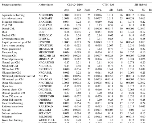
Table 1. Source category abbreviations with average CMAQ–DDM, CTM–RM, and SH (spatial hybrid) source contributions to PM2.5 concentrations for withheld CSN observation locations (N=75 observations) for January 2004. Note: all averages and standard deviations are expressed in µg m−3. Average total mass of withheld observations, and corresponding CMAQ–DDM, CTM–RM, and SH estimates were 11.7 (±8.3), 16.3 (±11), 8.59±4.7, and 9.2 (±5.7) µg m−3, respectively. NR=Non-road, CM=Combustion.
Source categories Abbreviation CMAQ–DDM CTM–RM SH Hybrid
Avg. SD Rank Avg. SD Rank Avg. SD Rank
Agricultural burning AGRIBURN 0.0040 0.003 25 0.0016 0.011 26 0.0012 0.0052 28 Aircraft emissions AIRCRAFT 0.0038 0.013 26 0.0037 0.013 25 0.0038 0.013 25 Biogenic emissions BIOGENIC 0.074 0.22 14 0.069 0.22 11 0.074 0.22 9 Coal CM COALCMB 0.16 0.39 9 0.15 0.38 4 0.15 0.38 3 Diesel CM. DIESELCM 0.00060 0.0017 30 0.0006 0.0017 30 0.0006 0.0017 30 Dust DUST 0.36 0.095 2 0.061 0.22 13 0.048 0.12 14 Fuel oil CM FUELOILC 0.14 0.54 12 0.14 0.62 6 0.14 0.63 5 Livestock emissions LIVEST2 0.31 0.89 3 0.31 0.85 1 0.31 0.88 1 Liquid petroleum gas CM LPGCMB 0.0043 0.013 24 0.0043 0.013 24 0.0043 0.013 24 Lawn waste burning LWASTEBU 0.10 0.032 13 0.018 0.067 21 0.010 0.026 22 Metal processing MEATALPR 0.18 0.16 7 0.12 0.70 7 0.064 0.22 12 Meat cooking MEATCOOK 0.034 0.089 19 0.034 0.10 16 0.032 0.10 17 Mexican CM MEXCMB_M 0.00070 0.0028 29 0.0007 0.0028 29 0.0007 0.0028 29 Mineral processing MINERALP 0.030 0.062 21 0.026 0.075 19 0.024 0.076 19 Natural gas CM NAGASCMB 0.17 0.21 8 0.11 0.36 8 0.078 0.20 8 NR diesel CM NRDIESEL 0.14 0.48 11 0.14 0.73 5 0.14 0.73 4 NR fuel oil CM NRFUELOI 0.010 0.036 23 0.010 0.041 23 0.010 0.039 23 NR gasoline CM NRGASOL 0.063 0.22 16 0.061 0.23 14 0.064 0.23 13 NR liquid petroleum Gas CM NRLPG 0.0014 0.0056 28 0.0014 0.0056 27 0.0014 0.0056 26 NR natural gas CM NRNAGAS 0.0005 0.0014 31 0.0005 0.0014 31 0.0005 0.0014 31 Other NR sources NROTHERS 0.0005 0.0012 32 0.0005 0.0012 32 0.0005 0.0012 32 Open fires OPENFIRE 0.15 0.099 10 0.021 0.11 20 0.017 0.10 20 Onroad diesel CM ORDIESEL 0.070 0.17 15 0.066 0.19 12 0.068 0.19 11 Onroad gasoline CM ORGASOL 0.27 0.60 4 0.20 0.54 2 0.24 0.62 2 Other CM sources OTHERCMB 0.040 0.072 18 0.029 0.14 18 0.026 0.11 18 Other PM sources OTHERS2 0.18 0.22 6 0.10 0.28 9 0.10 0.28 7 Prescribed burning PRESCRBU 0.032 0.054 20 0.031 0.24 17 0.032 0.24 16 Railroad emissions RAILROAD 0.013 0.046 22 0.013 0.046 22 0.013 0.045 21 Sea salt SEA SALT 0.0001 0.0005 33 0.0001 0.0005 33 0.00 0.0 33 Solvent emissions SOLVENT 0.051 0.094 17 0.044 0.14 15 0.040 0.13 15 Wildfires WILDFIRE 0.0018 0.0034 27 0.0012 0.0033 28 0.0013 0.00 27 Wood fuel burning WOOD FUEL 0.22 0.28 5 0.20 1.3 3 0.12 0.90 6 Wood stoves WOOD STOVE 0.62 0.44 1 0.083 0.29 10 0.069 0.28 10
period, coal combustion had the highest contribution to SO2
emissions (35080.3 metric tons per day) and the second high-est contribution to NOXemissions (14250.1 metric tons per day) behind mobile sources. The source impacts found here account for the transformation of these gaseous emissions from coal combustion.
Secondary formation processes increase the impact of coal combustion, biogenic and livestock emissions relative to their initial primary PM contribution. January 2004 pri-mary PM emissions estimates for biogenic and livestock were ranked 33rd and 31st, respectively. However, CMAQ– DDM, CTM–RM, and SH hybrid contributions ranked both sources significantly higher (biogenic rankings: 14th, 11th, and 9th, respectively; livestock rankings: 3rd, 1st, and 1st, respectively). Although primary PM2.5emissions from these
sources are not large, secondary processes and emissions from gaseous precursors led to high source contributions (Ta-ble S9). Biogenic sources emit large quantities of volatile organic compounds which go on to form secondary organic aerosols. Livestock emissions of gaseous ammonia react with sulfate, nitrate, and other acids to form ammonium salts. Therefore, the SH method captures and refines impacts from sources that contribute precursors of PM2.5.
3.3 Refined Spatial Fields
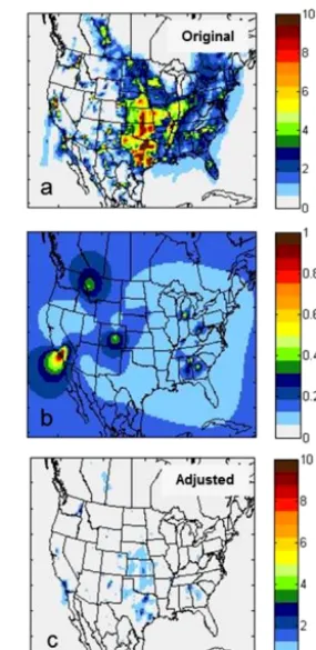
4 January 2004. Sources with high occurrences (∼> 50 %) of adjustment factors less than 1 include biomass burning, met-als processing, and natural gas combustion, and refined spa-tial fields for these sources are presented in the Supplement (Figs. S5–S7). Biomass burning includes impacts from agri-cultural burning, lawn waste burning, open fires, prescribed burning, wildfires, wood fuel burning, and wood stoves. The SH method significantly decreases impacts from biomass burning on 4 and 22 January in the eastern USA and for portions of the west coast (Fig. S5), largely driven by the observed potassium and organic compound (OC) levels be-ing lower than simulated levels. On average, CMAQ–DDM simulated levels were a factor of 3.1 (±1.1) times higher than SH values on 4 January, and a factor of 5.2 (±1.0) times higher on 22 January. Metal processing impacts were reduced for areas highly impacted by smelting and metal works industries including the Ohio River valley and mid-Atlantic regions (Fig. S6). On average, the CMAQ–DDM values were 21 (±21) % higher than SH values on 4 January, and 25 (±21) % higher on 22 January for metal process-ing impacts. Natural gas combustion impacts (area and point sources only) were reduced for the southeastern USA, the Ohio River valley region, the Gulf of Mexico states, and parts of California and Texas (Fig. S7). On average, CMAQ–DDM levels were 35 (±14) % higher than SH values on 4 January, and 72 (±28) % higher on 22 January for natural gas com-bustion impacts.
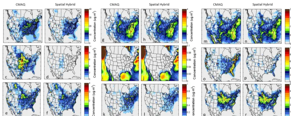
Refined spatial fields of January 2004 averaged source impacts are presented for eight sources: (c, d) dust, (e, f) on-road mobile sources, (g, h) coal combustion, (i, j) sea salt, (k, l) metal-related sources, (m, n) fuel oil combus-tion, (o, p) biomass burning, and (q, r) agricultural activities (Fig. 5). Total PM2.5concentration fields are also included
with overlapped observed concentrations from 28 January (a, b). The CMAQ–DDM spatial field overestimates concentra-tions in the Eastern USA, while overlapped concentraconcentra-tions agree more with spatial hybrid results. Modeled concentra-tions at monitors in mountainous areas, such as Salt Lake City, Utah, are underestimated due to local meteorological conditions (Gillies et al., 2010; Kelly et al., 2013). Winter-time temperature inversions, which cause stagnation in air circulation and consequently high air pollution episodes in industrial valleys, are challenging to capture in models.
Improved spatial field correlation is reflected in monthly averaged spatial fields (Fig. 5). SH dust impacts are greatly reduced domain-wide as compared to CMAQ–DDM. Monthly averaged refinement of biomass burning, where im-pacts were also greatly reduced, and metal-related source impact fields are consistent with results previously men-tioned for 4 and 22 January. Sea salt impacts are localized to coastal areas as expected, and agricultural activity most greatly impacts the mid-western USA, an area dominated by farm lands. Coal and fuel oil combustion impacts are highest in the eastern USA and western Mexico (fuel oil only) and
Figure 4. Hybrid-kriging adjustment of the dust impacts on PM2.5 on 22 January 2004: (a) original CMAQ–DDM simulation of dust source impacts; (b) spatial field of hybrid adjustment factors for dust (RjSH); (c) adjusted spatial field of dust source impacts.
were adjusted very little as compared to the original CMAQ– DDM field.
4 Discussion
The SH method uses observations and modeled concentra-tions of species to adjust impacts on a source-by-source ba-sis to provide spatially and temporally detailed source impact fields. The SH method also captures the impacts of secondary aerosol formation from precursor emission sources. Hybrid adjustment factors can be used to estimate the amount of change in emissions necessary for modeled results to better reflect observations, as emissions are roughly proportional to source impacts for primary sources (Hu et al., 2015). Krig-ing is an effective spatial interpolation method for spatially extending the CTM–RM model and generating spatial fields of adjustment factors. Kriging does not introduce significant error, as the adjusted fields maintain the spatial and tem-poral variability of the original fields, and this application led to simulated PM2.5mass concentrations being closer to
Figure 5. Average CMAQ–DDM and spatial hybrid source impacts on PM2.5for observation days in January 2004 for eight source cat-egories. Total PM2.5with overlapped PM2.5observations for 28 January (a, b). Impact of (c, d) soil/crustal material, (e, f) traffic-related sources, (g, h) coal combustion, (i, j) sea salt aerosol, (k, l) metal-related sources, (m, n) fuel oil combustion, (o, p) biomass burning, and agricultural activities (q, r).
chemistry. The SH method also improves simulated esti-mates of crustal and trace metal concentrations.
The SH method is being developed both to develop spa-tiotemporally accurate source impact fields that are con-sistent with observations, and also to provide an approach to increase our understanding of the spatiotemporal char-acteristics of source impacts in the United States. We find widespread adjustment to biomass burning and dust impacts (Rj less than 1). These source impacts are consistent with observations, emissions estimates, and atmospheric transport and transformation. The SH method is also novel in that, al-though some sources may not emit a certain pollutant, there still may be some interactions with emissions from other sources leading to those species being part of the source im-pact. For example, in the case of agricultural fertilizer emis-sions, although NOx is not directly emitted, the influence on nitrate concentrations is calculated. Although tradition-ally not quantified in receptor-oriented source apportionment methods, taking into account inter-source interactions is im-portant for determining the primary and secondary impacts of sources on air quality. This hybrid source- and receptor-oriented approach takes this into account and can determine impacts from elusive source interactions. However, this also shows that the formation of secondary species is often depen-dent upon multiple sources, and the impact of one source is dependent upon other sources, leading to ambiguity in source attribution. The approach here uses the sensitivities at cur-rent conditions, though also conducts a mass balance on a species-by-species basis minimizing any overall bias in the source impact attributions.
Spatial hybrid inputs, methods, and results have inher-ent uncertainties and challenges that are associated with im-plementation. Input uncertainties include measurement error and challenges are posed with temporal availability and spa-tial representativeness of concentrations. Emissions inputs for each source are available at different temporal and spa-tial scales. For instance point source emissions are available at hourly intervals in some cases, while dust emissions are highly variable, both spatially and temporally. Area source emissions are estimated at weekly or monthly intervals and averaged source fingerprints for the primary components of the PM2.5emissions are used, which removes the
consider-ation of locally varying source composition. Physical pro-cesses in CMAQ–DDM are uncertain as modeling atmo-spheric behavior is a complex undertaking. Also, first-order sensitivity approaches may not capture all nonlinearities in source-receptor relationships. SH results are also subject to potential systematic bias from the optimization and kriging steps, though our evaluation suggests those biases are mini-mal.
5 Conclusion
not a chemistry or physics model. It is a model based on statistics with the assumption that by incorporating obser-vations (truth) and modeled atmospheric processes (predic-tion), two results can be statistically combined together to yield a better approximation of source impacts. Efforts are continual for reducing uncertainties, increasing the time span of available results, and evaluating estimations with other data sources, such as satellite imagery and independent field measurements. In future studies, the model will be extended temporally to generate daily, adjusted spatial fields for the continental USA for multiple years and to develop improved source profiles for emissions characterization. Results from SH implementation are beneficial to policy makers, public health analysts, and other air quality scientists that use spa-tially and temporally complete source impact data in studies where outcomes influence human welfare.
The Supplement related to this article is available online at doi:10.5194/gmd-8-2153-2015-supplement.
Acknowledgements. This publication was made possible in part
by USEPA STAR grants R833626, R833866, R834799 and RD83479901, STAR Fellowship FP-91761401-0, and by NASA under grant NNX11AI55G. Its contents are solely the responsibility of the grantee and do not necessarily represent the official views of the US government. Further, US government does not endorse the purchase of any commercial products or services mentioned in the publication. We also acknowledge the Southern Company and the Alfred P. Sloan Foundation for their support and thank Eric Edgerton of ARA, Inc. for access to the SEARCH data.
Edited by: A. Colette
References
Baker, K. R., Simon, H., and Kelly, J. T.: Challenges to Modeling “Cold Pool” Meteorology Associated with High Pollution Episodes, Environ. Sci. Technol., 45, 7118–7119, doi:10.1021/Es202705v, 2011.
Balachandran, S., Pachon, J. E., Hu, Y. T., Lee, D., Mulhol-land, J. A., and Russell, A. G.: Ensemble-trained source apportionment of fine particulate matter and method uncertainty analysis, Atmos. Environ., 61, 387–394, doi:10.1016/j.atmosenv.2012.07.031, 2012.
Balachandran, S., Chang, H. H., Pachon, J. E., Holmes, H. A., Mulholland, J. A., and Russell, A. G.: Bayesian-Based Ensem-ble Source Apportionment of PM2.5, Environ. Sci. Technol., 47, 13511–13518, doi:10.1021/Es4020647, 2013.
Bell, M. L.: The use of ambient air quality modeling to estimate individual and population exposure for human health research: A case study of ozone in the Northern Georgia Region of the United States, Environ. Int., 32, 586–593, 2006.
Binkowski, F. S. and Roselle, S. J.: Models-3 Community Multi-scale Air Quality (CMAQ) model aerosol compo-nent: 1. Model description, J. Geophys. Res., 108, 4183, doi:10.1029/2001JD001409, 2003.
Byun, D. and Schere, K. L.: Review of the governing equations, computational algorithms, and other components of the models-3 Community Multiscale Air Quality (CMAQ) modeling system, Appl. Mech. Rev., 59, 51–77, doi:10.1115/1.2128636, 2006. Campen, M. J., Nolan, J. P., Schladweiler, M. C. J., Kodavanti, U. P.,
Evansky, P. A., Costa, D. L., and Watkinson, W. P.: Cardiovascu-lar and thermoregulatory effects of inhaled PM-associated transi-tion metals: A potential interactransi-tion between nickel and vanadium sulfate, Toxicol. Sci., 64, 243–252, doi:10.1093/toxsci/64.2.243, 2001.
Carter, W. P. L.: Documentation of the SAPRC-99 Chemical Mech-anism for VOC Reactivity Assessment, Contract No. 92-329 and 95-308, California Air Resources BoardUniversity of California, Riverside, USA, 2000.
CEP: Sparse Matrix Operator Kernel Emissions Modeling System (SMOKE) User Manual, Carolina Environmental Program – The University of North Carolina at Chapel Hill, Chapel Hill, NC, USA, 2003.
Chow, J. C., Watson, J. G., Pritchett, L. C., Pierson, W. R., Fra-zier, C. A., and Purcell, R. G.: The Dri Thermal Optical Re-flectance Carbon Analysis System - Description, Evaluation and Applications in United-States Air-Quality Studies, Atmos. Envi-ron. A-Gen., 27, 1185–1201, doi:10.1016/0960-1686(93)90245-T, 1993.
Darrow, L. A., Klein, M., Strickland, M. J., Mulholland, J. A., and Tolbert, P. E.: Ambient Air Pollution and Birth Weight in Full-Term Infants in Atlanta, 1994–2004, Environ. Health Persp., 119, 731–737, doi:10.1289/Ehp.1002785, 2011.
Dominici, F., Peng, R. D., Barr, C. D., and Bell, M. L.: Protect-ing Human Health From Air Pollution ShiftProtect-ing From a SProtect-ingle- Single-pollutant to a MultiSingle-pollutant Approach, Epidemiology, 21, 187– 194, doi:10.1097/Ede.0b013e3181cc86e8, 2010.
Dunker, A. M.: Efficient Calculation of Sensitivity Coefficients for Complex Atmospheric Models, Atmos. Environ., 15, 1155– 1161, doi:10.1016/0004-6981(81)90305-X, 1981.
Dunker, A. M.: The Decoupled Direct Method for Calculating Sen-sitivity Coefficients in Chemical-Kinetics, J. Chem. Phys., 81, 2385–2393, doi:10.1063/1.447938, 1984.
Fletcher, R.: Practical Methods of Optimization, John Wiley and Sons, Cornwall, UK, 1987.
Gill, P. E., Murray, W., and Wright, M. H.: Practical Optimization, Academic Press, London, UK, 1981.
Gillies, R. R., Wang, S. Y., and Booth, M. R.: Atmospheric Scale Interaction on Wintertime Intermountain West Low-Level Inver-sions, Weather Forecast., 25, 1196–1210, 2010.
Grell, G., Dudhia, J., and Stauffer, D.: A description of the Fifth-Generation Penn State/NCAR Mesoscale Model (MM5), NCAR Technical Note: NCAR/TN-398CSTRNCAR/TN 398CSTR, Boulder, Colorado, USA, 1994.
Hanna, S. R., Lu, Z. G., Frey, H. C., Wheeler, N., Vukovich, J., Arunachalam, S., Fernau, M., and Hansen, D. A.: Uncer-tainties in predicted ozone concentrations due to input uncer-tainties for the UAM-V photochemical grid model applied to the July 1995 OTAG domain, Atmos. Environ., 35, 891–903, doi:10.1016/S1352-2310(00)00367-8, 2001.
Hansen, D. A., Edgerton, E. S., Hartsell, B. E., Jansen, J. J., Kan-dasamy, N., Hidy, G. M., and Blanchard, C. L.: The southeastern aerosol research and characterization study: Part 1 – overview, J. Air Waste Manage., 53, 1460–1471, 2003.
Hansen, D. A., Edgerton, E., Hartsell, B., Jansen, J., Burge, H., Koutrakis, P., Rogers, C., Suh, H., Chow, J., Zielinska, B., Mc-Murry, P., Mulholland, J., Russell, A., and Rasmussen, R.: Air quality measurements for the aerosol research and inhalation epi-demiology study, J. Air Waste Manage., 56, 1445–1458, 2006. Henry R. C.: Duality in multivariate receptor models, Chemometr.
Intell. Lab., 77, 59–63, 2005.
Hu, Y., Odman, M. T., and Russell, A. G.: Mass conservation in the Community Multiscale Air Quality model, Atmos. Environ., 40, 1199–1204, 2006.
Hu, Y., Balachandran, S., Pachon, J. E., Baek, J., Ivey, C., Holmes, H., Odman, M. T., Mulholland, J. A., and Russell, A. G.: Fine particulate matter source apportionment using a hybrid chemical transport and receptor model approach, Atmos. Chem. Phys., 14, 5415–5431, doi:10.5194/acp-14-5415-2014, 2014.
Hu, Y., Odman, M. T., Chang, M. E., and Russell, A. G.: Opera-tional forecasting of source impacts for dynamic air quality man-agement, Atmos. Environ., doi:10.1016/j.atmosenv.2015.04.061, in press, 2015.
Kelly, K. E, Kotchenruther, R., Kuprov, R., and Silcox, G. D.: Re-ceptor model source attributions for Utah’s Salt Lake City air-shed and the impacts of wintertime secondary ammonium nitrate and ammonium chloride aerosol, J. Air Waste Manage., 63, 575– 590, 2013.
Koo, B., Wilson, G. M., Morris, R. E., Dunker, A. M., and Yarwood, G.: Comparison of Source Apportionment and Sensitivity Analy-sis in a Particulate Matter Air Quality Model, Environ. Sci. Tech-nol., 43, 6669–6675, 2009.
Laden, F., Neas, L. M., Dockery, D. W., and Schwartz, J.: Associ-ation of fine particulate matter from different sources with daily mortality in six US cities, Environ. Health Persp., 108, 941–947, doi:10.1289/Ehp.00108941, 2000.
Lim, S. S., Vos, T., Flaxman, A. D., et al.: A comparative risk as-sessment of burden of disease and injury attributable to 67 risk factors and risk factor clusters in 21 regions, 1990–2010: a sys-tematic analysis for the Global Burden of Disease Study 2010, Lancet, 380, 2224–2260, 2012.
Marmur, A., Park, S. K., Mulholland, J. A., Tolbert, P. E., and Rus-sell, A. G.: Source apportionment of PM2.5in the southeastern United States using receptor and emissions-based models: Con-ceptual differences and implications for time-series health stud-ies, Atmos. Environ., 40, 2533–2551, 2006.
Maykut, N. N., Lewtas, J., Kim, E., and Larson, T. V.: Source appor-tionment of PM2.5at an urban IMPROVE site in Seattle, Wash-ington, Environ. Sci. Technol., 37, 5135–5142, 2003.
Napelenok, S. L., Cohan, D. S., Hu, Y. T., and Russell, A. G.: Decoupled direct 3D sensitivity analysis for particu-late matter (DDM-3D/PM), Atmos. Environ., 40, 6112–6121, doi:10.1016/j.atmosenv.2006.05.039, 2006.
Oberdorster, G., Oberdorster, E., and Oberdorster, J.: Nan-otoxicology: An emerging discipline evolving from studies of ultrafine particles, Environ. Health Persp., 113, 823–839, doi:10.1289/Ehp.7339, 2005.
Pattero, P. and Tapper, U.: Positive Matrix Factorization – a Nonnegative Factor Model with Optimal Utilization of Error-Estimates of Data Values, Environmetrics, 5, 111–126, 1994. Peel, J. L., Klein, M., Flanders, W. D., Mulholland, J. A., Freed, G.,
and Tolbert, P. E.: Ambient Air Pollution and Apnea and Brady-cardia in High-Risk Infants on Home Monitors, Environ. Health Persp., 119, 1321–1327, doi:10.1289/Ehp.1002739, 2011. Peters, A., Wichmann, H. E., Tuch, T., Heinrich, J., and Heyder, J.:
Respiratory effects are associated with the number of ultrafine particles, Am. J. Resp. Crit. Care, 155, 1376–1383, 1997. Pleim, J. E. and Xiu, A.: Development and Testing of a
Sur-face Flux and Planetary Boundary-Layer Model for Appli-cation in Mesoscale Models, J. Appl. Meteorol., 34, 16–32, doi:10.1175/1520-0450-34.1.16, 1995.
Pope, C. A., Burnett, R. T., Thun, M. J., Calle, E. E., Krewski, D., Ito, K., and Thurston, G. D.: Lung cancer, cardiopul-monary mortality, and long-term exposure to fine particulate air pollution, JAMA – J. Am. Med. Assoc., 287, 1132–1141, doi:10.1001/jama.287.9.1132, 2002.
Reff, A., Bhave, P. V., Simon, H., Pace, T. G., Pouliot, G. A., Mob-ley, J. D., and Houyoux, M.: Emissions Inventory of PM2.5Trace Elements across the United States, Environ. Sci. Technol., 43, 5790–5796, doi:10.1021/Es802930x, 2009.
Samet, J. M., Dominici, F., Curriero, F. C., Coursac, I., and Zeger, S. L.: Fine particulate air pollution and mortality in 20 US Cities, 1987–1994, New Engl. J. Med., 343, 1742–1749, doi:10.1056/Nejm200012143432401, 2000.
Sarnat, J. A., Marmur, A., Klein, M., Kim, E., Russell, A. G., Sar-nat, S. E., Mulholland, J. A., Hopke, P. K., and Tolbert, P. E.: Fine particle sources and cardiorespiratory morbidity: An appli-cation of chemical mass balance and factor analytical source-apportionment methods, Environ. Health Persp., 116, 459–466, doi:10.1289/Ehp.10873, 2008.
Schauer, J. J. and Cass, G. R.: Source apportionment of wintertime gas-phase and particle-phase air pollutants using organic com-pounds as tracers, Environ. Sci. Technol., 34, 1821–1832, 2000. Seigneur, C., Pun, B., Pai, P., Louis, J. F., Solomon, P., Emery, C., Morris, R., Zahniser, M., Worsnop, D., Koutrakis, P., White, W., and Tombach, I.: Guidance for the performance evaluation of three-dimensional air quality modeling systems for particulate matter and visibility, J. Air Waste Manage., 50, 588–599, 2000. Thurston, G. D., Ito, K., Mar, T., Christensen, W. F., Eatough, D.
J., Henry, R. C., Kim, E., Laden, F., Lall, R., Larson, T. V., Liu, H., Neas, L., Pinto, J., Stolzel, M., Suh, H., and Hopke, P. K.: Workgroup report: Workshop on source apportionment of particulate matter health effects – Intercomparison of re-sults and implications, Environ. Health Persp., 113, 1768–1774, doi:10.1289/Ehp.7989, 2005.
Tolbert, P. E., Klein, M., Peel, J. L., Sarnat, S. E., and Sarnat, J. A.: Multipollutant modeling issues in a study of ambient air quality and emergency department visits in Atlanta, J. Expo. Sci. Env. Epid., 17, S29–S35, doi:10.1038/sj.jes.7500625, 2007.
community-based study, Environ. Health Persp., 105, 514–520, doi:10.1289/Ehp.97105514, 1997.
Watson, J. G., Cooper, J. A., and Huntzicker, J. J.: The Effective Variance Weighting for Least-Squares Calculations Applied to the Mass Balance Receptor Model, Atmos. Environ., 18, 1347– 1355, doi:10.1016/0004-6981(84)90043-X, 1984.
Watson, J. G., Chow, J. C., and Fujita, E. M.: Review of volatile organic compound source apportionment by chemical mass bal-ance, Atmos. Environ., 35, 1567–1584, 2001.
Xiu, A. J. and Pleim, J. E.: Development of a land surface model. Part I: Application in a mesoscale meteorological model, J. Appl. Meteorol., 40, 192–209, doi:10.1175/1520-0450(2001)040<0192:Doalsm>2.0.Co;2, 2001.