www.geosci-model-dev.net/5/523/2012/ doi:10.5194/gmd-5-523-2012
© Author(s) 2012. CC Attribution 3.0 License.
Geoscientific
Model Development
Pre-industrial and mid-Pliocene simulations with NorESM-L
Z. S. Zhang1,2,3, K. Nisancioglu1,2, M. Bentsen1,2, J. Tjiputra1,2, I. Bethke1,2, Q. Yan3, B. Risebrobakken1,2, C. Andersson1,2, and E. Jansen1,2
1Bjerknes Centre for Climate Research, Allegaten 55, 5007, Bergen, Norway 2UNI Research, Allegaten 55, 5007, Bergen, Norway
3Nansen-Zhu International Research Center, Institute of Atmospheric Physics, Chinese Academy of Sciences,
100029, Beijing, China
Correspondence to: Z. S. Zhang (zhongshi.zhang@bjerknes.uib.no)
Received: 20 December 2011 – Published in Geosci. Model Dev. Discuss.: 13 January 2012 Revised: 3 April 2012 – Accepted: 3 April 2012 – Published: 25 April 2012
Abstract. The mid-Pliocene period (3.3 to 3.0 Ma) is known as a warm climate with atmospheric greenhouse gas levels similar to the present. As the climate at this time was in equilibrium with the greenhouse forcing, it is a valuable test case to better understand the long-term response to high lev-els of atmospheric greenhouse gases. In this study, we use the low resolution version of the Norwegian Earth System Model (NorESM-L) to simulate the pre-industrial and the mid-Pliocene climate. Comparison of the simulation with observations demonstrates that NorESM-L simulates a re-alistic pre-industrial climate. The simulated mid-Pliocene global mean surface air temperature is 16.7◦C, which is 3.2◦C warmer than the pre-industrial. The simulated mid-Pliocene global mean sea surface temperature is 19.1◦C, which is 2.0◦C warmer than the pre-industrial. The warming is relatively uniform globally, except for a strong amplifica-tion at high latitudes.
1 Introduction
The Pliocene period, also referred to as the mid-Piacenzian, is known as the most recent period in Earth’s his-tory when the global average temperature was warmer than today. Estimates are on the order of 2–3◦C warmer com-pared to today (Jansen et al., 2007; Dowsett et al., 2010). This warming is accompanied by a global sea level that was 10–45 m higher than present (e.g. Raymo et al., 1996). The warming is within the range of the Intergovernmental Panel on Climate Change (IPCC) projections of global temperature increases for the 21st century (Meehl et al., 2007). Unlike
other warm geological periods, e.g. Eocene and Miocene, the paleogeography of the mid-Pliocene is similar to the present. Thus, the mid-Pliocene climate has been considered as an analog for the long-term fate of the climate system under the present level of greenhouse gases forcing.
The mid-Pliocene has been a focus for several data syn-theses (e.g. Dowsett et al., 1994, 1996, 1999, 2009, 2010) and modelling (e.g. Chandler et al., 1994; Sloan et al., 1996; Haywood et al., 2000; Haywood and Valdes, 2004; Jiang et al., 2005; Yan et al., 2011). However, early model studies in-dicated a clear model-data discrepancy. Interpretation of the proxy data suggested that the Atlantic Meridional Overturn-ing Circulation (AMOC) was stronger in the mid-Pliocene compared to the present (Raymo et al., 1996; Ravelo and An-dreasen, 2000; Hodell and Venz-Curtis, 2006). The enhanced AMOC was thought to have led to increased northward heat transport and warm temperatures in the high latitude Atlantic and Arctic (Dowsett et al., 1992, 2009). However, most cli-mate models forced with mid-Pliocene boundary conditions did not simulate a stronger AMOC and enhanced heat trans-port (e.g. Haywood and Valdes, 2004; Yan et al., 2011). Thus, to better understand the dynamics behind the esti-mated high latitude warmth of the mid-Pliocene, and to as-sess the ability of climate models in simulating a past warm climate, the Pliocene Paleoclimate Modeling Intercompari-son Project (PlioMIP) was recently initiated (Haywood et al., 2010, 2011).
Climate Centre (NCC) to the PlioMIP experiment II. The NorESM-L model is introduced in detail in Sect. 2. Section 3 describes the experimental design and Sect. 4 discusses the results. A brief discussion and summary are given in Sect. 5.
2 Model description
The NorESM is an Earth system model built under the struc-ture of the Community Earth System Model (CESM) from the National Center for Atmospheric Research (NCAR). It uses the same coupler (CLP7), atmosphere (CAM4), land (CLM4), and sea ice (CICE4) components as the CESM. The key difference to the standard CESM configu-ration is an optional modification of the treatment of atmo-spheric chemistry, aerosols, and clouds (Seland et al., 2008) and the ocean component, which is the Miami Isopycnic Co-ordinate Ocean Model (MICOM) in the NorESM. Simula-tions with the NorESM are the contribuSimula-tions from the Nor-wegian Climate Centre (NCC) to the Coupled Model Inter-comparison Project Phase 5 (CMIP5), which is expected to be included in the upcoming Intergovernmental Panel on Cli-mate Change (IPCC) Fifth Assessment Report (AR5).
In this study we use the low resolution version of the NorESM (NorESM-L). The horizontal resolution for the at-mosphere is T31, with 26 levels in the vertical. This cor-responds roughly to a grid size of approximately 3.75◦C. The horizontal resolution of the ocean is g37, correspond-ing to a nominal grid size of 3◦C. The ocean component has 30 isopycnic layers in the vertical. Detailed documentations for each component of the model system are given in the fol-lowing sections.
2.1 Atmospheric model
The atmosphere component of the NorESM-L is the spectral Community Atmosphere Model CAM4 (Neale et al., 2010; Eaton, 2010). It uses the Eulerian dynamical core, which is based on the hybrid vertical coordinate developed by Sim-mons and Str¨ufing (1981). The model includes physical pa-rameterizations of convection, clouds, surface processes, and turbulent mixing. The parameterization of deep convection uses the scheme developed by Zhang and McFarlane (1995), together with the convective momentum transport modifica-tion developed by Richter and Rasch (2008), and the dilute plume modification developed by Raymond and Blyth (1986, 1992). The parameterization of clouds uses the scheme in-troduced by Slingo (1987), with the variations described by Hack et al. (1993), Kiehl et al. (1998), and Rasch and Kristj´ansson (1998). The parameterization of surface pro-cesses uses a bulk exchange formulation described by Neale et al. (2010) to calculate the surface exchange of heat, mois-ture and momentum between the atmosphere and land, ocean or ice surfaces. The parameterization of turbulence includes the scheme of free atmosphere turbulent diffusivities and the
scheme of non-local atmospheric boundary layer parameter-ization described by Holtslag and Boville (1993) and Neale et al. (2010). The standard CAM4 treatment of atmospheric chemistry, aerosols, and clouds is used in this study. Detailed introductions to CAM4 can be found in the scientific descrip-tion of CAM4 (Neale et al., 2010) and the user guide (Eaton, 2010).
2.2 Land model
The land component used in NorESM-L is the Community Land Model CLM4 (Oleson et al., 2010; Kluzek, 2011). It calculates radiation and heat fluxes at the land-atmosphere interface, as well as temperature, humidity, and soil thermal and hydrologic states. The sub-grid scale surface heterogene-ity is represented through fractional coverage of glacier, lake, wetland, urban, and vegetation consisting of up to 15 plant functional types (PFTs) plus bare ground. Soil colours in the model are fitted to a range of 20 soil classes. The radiation fluxes are calculated according to the formulation introduced by Oleson et al. (2010). The heat fluxes are calculated using the Monin-Obukhov similarity theory as described by Zeng et al. (1998). Soil and snow temperatures are calculated ac-cording to the numerical solution introduced by Oleson et al. (2010). The model calculates changes in canopy water, snow water, soil water, and soil ice and water. A river trans-port model is included to give a closed hydrological cycle. Detailed descriptions of CLM4 can be found in the technical description (Oleson et al., 2010) and the user guide (Kluzek, 2011).
2.3 Sea ice model
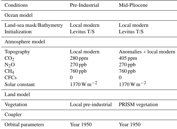
Table 1. Boundary and initial conditions for the pre-industrial and the mid-Pliocene experiment.
Conditions Pre-Industrial Mid-Pliocene
Ocean model
Land-sea mask/Bathymetry Local modern Local modern Initialization Levitus T/S Levitus T/S
Atmosphere model
Topography Local modern Anomalies + local modern
CO2 280 ppm 405 ppm
N2O 270 ppb 270 ppb
CH4 760 ppb 760 ppb
CFCs 0 0
Solar constant 1370 W m−2 1370 W m−2
Land model
Vegetation Local pre-industrial PRISM vegetation
Coupler
Orbital parameters Year 1950 Year 1950
2.4 Ocean model
The ocean component used in the NorESM-L is based on the Miami Isopycnic Coordinate Ocean Model MICOM (Bleck and Smith, 1990; Bleck et al., 1992), which uses potential density as vertical coordinate. The model consists of a stack of 30 isopycnal layers evaluated against a reference pressure of 2000 db, and a mixed layer on top represented by two non-isopycnal layers, providing the linkage between the atmo-spheric forcing and the ocean interior. Modifications of the original MICOM have been prompted by the desire to im-prove conservation of mass, heat, and tracers and to imple-ment robust, accurate, and efficient transport of many trac-ers, which is particularly important for ocean biogeochem-istry modelling. Furthermore, the pressure gradient force is now accurately estimated using in situ density, the diapyc-nal diffusion equation is solved by an implicit method, and numerous physical parameterizations have been improved or added in order to reduce model biases particular in coupled climate model configurations. These changes are described by Assmann et al. (2010) and Alterskjær et al. (2012).
3 Experimental designs
3.1 Pre-industrial control experiment
Following the PlioMIP experimental guidelines (Haywood, et al., 2011), the pre-industrial control experiment presented in this paper uses the modern land-sea mask, topography, and the ice sheets and vegetation for year 1850 (Table 1). All these geographic boundary conditions are taken from the CESM (Vertenstein et al., 2010). The ocean model
uses the modern bathymetry and is initialized from Levitus temperature and salinity (Levitus and Boyer, 1994). Atmo-spheric greenhouse gases are set to the pre-industrial values of 280 ppm CO2, 270 ppb N2O, 760 ppb CH4, and zero levels
of CFCs. The solar constant is set to 1370 W m−2. Orbital
parameters are set to the values for 1950 (Berger, 1978). The pre-industrial aerosol conditions from the CESM (Verten-stein et al., 2010) are used in the pre-industrial control exper-iment. With these boundary conditions and initial conditions, the pre-industrial control experiment is run for 1500 yr.
3.2 Mid-Pliocene experiment
13.2 13.6 14 14.4 14.8
15.2 15.6 16 16.4 16.8
0 500 1000 1500
-0.5 0 0.5 1 1.5
10 15 20 25 30
(a)
(b)
(c) TOA
TS
AMOC
Energy (W/m )
T
emperature ( C)
A
MOC (Sv)
2
o
Year
Fig. 1. Time series for (a) the energy balance at the top of NorESM-L (W m−2), (b) surface temperature (◦C), and (c) the maximum of the Atlantic overturning stream function (Sv) in the pre-industrial (red) and the mid-Pliocene experiment (blue). The thin lines show annual mean values and the bold lines show 21-yr running averages.
opened. Furthermore, the PRISM DOT deep ocean tempera-ture (Dowsett et al., 2009) is not used to initialize the ocean model in the mid-Pliocene experiment. Due to the complex-ity in the grid system, the initial depth of each isopycnic layer has to be reestimated, if the initial temperature and salinity are changed. These changes largely modify the initial ocean stratification. In order to avoid the large modifications in the initial ocean stratification, the initial conditions, which are identical to the industrial experiment, are used in the pre-industrial experiment.
The PRISM Pliocene topography file topo v1.3 (Sohl et al., 2009) is used to build the topography for the experi-ment. The difference between PRISM Pliocene topography and PRISM modern topography is interpolated to the T31 resolution. Then, the interpolated difference is added to the modern topography used in the pre-industrial experiment.
The PRISM Pliocene vegetation biome veg v1.2 (Hill et al., 2007; Salzmann et al., 2008) is used to construct the veg-etation and ice sheets for the mid-Pliocene experiment. The PRISM Pliocene vegetation is interpolated to the T31 resolu-tion. Subsequently, the biome vegetation types are changed to the LSM (Land System Model) vegetation types, accord-ing to the table named Biome4 conversion to LSM edited by Rosenbloom (2009). Finally, the LSM vegetation file is con-verted to appropriate boundary conditions for the CLM using the CCSM paleoclimate tools from NCAR (Rosenbloom et al., 2010).
Table 2. Global mean value for the pre-industrial and the mid-Pliocene experiment.
Exp. Pre-industrial Mid-Pliocene
Top energy balance 0.04 W m−2 0.13 W m−2 Surface temperature 13.5◦C 16.7◦C Precipitation 2.7 mm d−1 2.9 mm d−1 Sea surface temperature 17.1◦C 19.1◦C Maximum AMOC 21.8 Sv 23.4 Sv
For the greenhouse gases, the atmospheric CO2 level is
set to 405 ppm. Other greenhouse gases are kept at the same levels as those in the pre-industrial control experiment. Other boundary conditions, including solar constant, orbital param-eters and aerosols, are also kept at the same levels as the pre-industrial control experiment.
3.3 Time integration
The pre-industrial and mid-Pliocene experiments are both run for 1500 yr. Time series of the top of the atmosphere en-ergy balance, global mean surface air temperature and max-imum Atlantic meridional overturning circulation (AMOC) are shown in Fig. 1. Both experiments reach an equilibrium state after approximately 1000 yr of model integration time. In this paper we calculate the climatological means from the last 200 yr of each simulation.
4 Results
4.1 Pre-industrial control experiment
4.1.1 Surface air temperature
For the pre-industrial experiment, the global annual mean surface air temperature (SAT) is 13.5◦C (Table 2, Fig. 1), in good agreement with pre-industrial temperature estimates (e.g. Hansen et al., 2010). The zonal mean SAT (Fig. 2a) shows that the annual mean temperature at the North Pole is about −20◦C, whereas it is −44◦C close to the South Pole. The warmest temperatures are found over the western tropical Pacific and eastern tropical Indian Ocean, with tem-peratures higher than 28◦C (Fig. 3a). The coldest tempera-tures are found over East Antarctica, with temperatempera-tures be-low−50◦C. The zero degree isotherm in the Southern Hemi-sphere is relatively zonal and located close to 60◦S. In con-trast, the zero degree isotherm in the Northern Hemisphere is strongly influenced by topography and land-sea distribu-tion. It is located close to 70◦N over the Labrador Sea and the Norwegian Sea, and close to 60◦N in the North Pacific.
-90 -60 -30 0 30 60 90 0
2 4 6 8
-90 -60 -30 0 30 60 90
-50 -40 -30 -20 -10 0 10 20 30
(a) (b)
T
emperature ( C)
Precipitation (mm/d)
o
Latitude Latitude
Pre-Industrial Mid-Pliocene ERAint 79-08
Pre-Industrial Mid-Pliocene GPCP 79-08
Fig. 2. Zonal mean surface temperature (a, ◦C) and precip-itation (b, mm d−1) for the observations (gray lines), the pre-industrial experiment (red lines) and the mid-Pliocene experiment (blue lines). The temperature observation is ERA-interim tem-perature from 1979 to 2008. The precipitation observation is the 1979–2008 precipitation from the Global Precipitation Climatology Project (GPCP).
temperatures are slightly colder than the modern estimates represented by the ERA-interim data.
4.1.2 Precipitation
In the industrial experiment, the global annual mean pre-cipitation is 2.7 mm day−1 (Table 2), with a peak in annual zonal mean precipitation in the Intertropical Convergence Zone (ITCZ) of about 6.5 mm day−1(Fig. 2b). The lowest precipitation, about 0.2 mm day−1, appears close to the South Pole. Regionally (Fig. 3c), high precipitation can be seen over the tropical ocean and continent, with annual mean pre-cipitation higher than 12 mm day−1over the western tropical Pacific. In the Sahara and over East Antarctica, precipitation is less than 0.2 mm day−1.
Compared to the observed precipitation data from the Global Precipitation Climatology Project (GPCP; Adler et al., 2003) averaged over the period 1979–2008 (Fig. 3d), the overall pattern and amount are in good agreement. How-ever, model-data discrepancies exist in the tropics and in the Southern Hemisphere sub-tropical oceans, where the simu-lated precipitation is higher than the observations.
4.1.3 Sea surface temperature
In the pre-industrial experiment, the global annual mean SST is 17.1◦C (Table 2), with the warmest temperatures, higher than 28◦C, in the western tropical Pacific and eastern tropical Indian Ocean (Fig. 4a). The zero degree isotherm is located close to 60◦S in the Southern Hemisphere and around the margin of the Arctic in the Northern Hemisphere.
The simulated SSTs compare well with the data of Levitus and Boyer (1994, Fig. 4b). However, the model simulations are slightly cooler than the observations, in particular in the tropical oceans. This is expected, as the observations repre-sent today’s SST and not pre-industrial values.
4.1.4 Sea surface salinity
High sea surface salinity occurs generally at the surface of the subtropical oceans (Fig. 4c). Salinity is relatively low at the surface of the tropical and high latitude oceans. The high-est salinities, close to 38 g kg−1, appear at the surface of the
Mediterranean Sea. The lowest salinities, with salinity less than 32 g kg−1, occur at the surface of marginal seas in the
Arctic, the Hudson Bay (northeastern North America), the Gulf of Guinea (eastern tropical Atlantic) and the Indonesian archipelago (western tropical Pacific).
The global sea surface pattern (Fig. 4d) agrees well with observations (Levitus and Boyer, 1994). However, simulated salinities are a little lower than observed values at the surface of the Atlantic Ocean, but higher in the Arctic and the North Pacific.
4.2 Mid-Pliocene experiment
4.2.1 Surface air temperature
In the mid-Pliocene experiment, the global annual mean SAT is 16.7◦C (Table 2, Fig. 1). The zonal mean annual SAT shows that the annual mean temperature close to the South Pole is about−40◦C, whereas it is about−7◦C close to the North Pole (Fig. 2a). The annual mean temperature is about 27◦C at the equator.
Compared to the pre-industrial control run, the simulated mid-Pliocene global annual mean SAT is 3.2◦C warmer. Warming occurs almost globally (Fig. 5a), with stronger warming appearing in high latitudes. Cooler temperatures are simulated over parts of the western tropical Pacific, the Southern Ocean close to West Antarctica, tropical Africa, East Australia, and East Antarctica.
The warming can also be seen in the seasonal SAT anoma-lies between the mid-Pliocene and the pre-industrial. In bo-real summer (Fig. 5b), the warming exceeds 5◦C over Green-land in the Northern Hemisphere and around the margin of Antarctica in the Southern Hemisphere. In boreal winter (Fig. 5c), the middle and high latitude continents are signif-icantly warmer in the Northern Hemisphere, with a temper-ature increase during the mid-Pliocene of more than 5◦C. The warming increases northward towards the North Pole, where temperatures increase as much as 20◦C. In the South-ern Hemisphere, the strongest warming occurs around the Antarctic margin, with temperatures increasing more than 5◦C.
4.2.2 Precipitation
90N
90S EQ
90N
90S EQ
0 180 360
(a)
(b)
-50 -40 24 20 16 12 8 4 0 -10 -20 -30 32 28
-50 -40 24 20 16 12 8 4 0 -10 -20 -30 32 28
90N
90S EQ
90N
90S EQ
0 180 360
(c)
(d)
0.2 0.5 10 9 8 7 6 5 4 3 2 1 14 12 16
0.2 0.5 10 9 8 7 6 5 4 3 2 1 14 12 16
Fig. 3. Simulated annual mean pre-industrial surface temperature (a,◦C) and precipitation (c, mm d−1), in comparison to ERA-interim 1979–2008 surface temperature (b,◦C) and GPCP 1979–2008 precipitation (d, mm d−1).
-2 0 24 22 20 18 16 14 12 10 8 4 30 28 26 90N
90S EQ
90N
90S EQ
0 180 360
(a)
(b) Pre-Industrial SST
Levitus SST -2
0 24 22 20 18 16 14 12 10 8 4 30 28 26
90N
90S EQ
90N
90S EQ
0 180 360
(c)
(d) 32.0 33.0 37.2 36.8 36.4 36.0 35.6 35.2 34.8 34.4 34.0 33.5 38.0 37.6 32.0 33.0 37.2 36.8 36.4 36.0 35.6 35.2 34.8 34.4 34.0 33.5 38.0 37.6
Pre-Industrial SSS
Levitus SSS
90N
90S EQ
90N
90S EQ
90N
90S EQ
90N
90S EQ
90N
90S EQ
90N
90S EQ
0 180 360 0 8 16 24
(a)
(b)
(c)
ANN
JJA
DJF
Fig. 5. Temperature differences (◦C) between the mid-Pliocene and the pre-industrial experiment, (a) for annual mean, (b) for boreal summer and (c) for boreal winter. The bold lines on the right sides show zonal mean values.
Compared to the pre-industrial experiment, the simulated mid-Pliocene global annual mean precipitation increases by about 0.2 mm day−1. Precipitation increases in the tropics north of the equator by 1 mm day−1, and in the middle and high latitudes of both hemispheres by 0.5 mm day−1. Pre-cipitation decreases in the subtropics of the Northern Hemi-sphere by 0.1 mm day−1, and tropics of the Southern
Hemi-sphere (Fig. 6a) by 0.9 mm day−1. The differences similar to
those of the zonal mean annual precipitation are also simu-lated in the seasonal precipitation anomalies (Fig. 6b and c).
4.2.3 Sea surface temperature
In the mid-Pliocene experiment (Fig. 7a), the warmest ocean surfaces with temperature higher than 28◦C appear in the tropical Indian Ocean, the western tropical Pacific, the east-ern tropical Pacific and the easteast-ern tropical Atlantic. The zero degree isotherm almost disappears in the Southern Hemi-sphere. In the Northern Hemisphere, it is located further
90N
90S EQ
90N
90S EQ
90N
90S EQ
90N
90S EQ
90N
90S EQ
90N
90S EQ
0 180 360 -2 -1 0 2
(a)
(b)
(c)
ANN
JJA
DJF
1
Fig. 6. Precipitation differences (mm d−1) between the mid-Pliocene and the pre-industrial experiment, (a) for annual mean, (b) for boreal summer and (c) for boreal winter. The bold lines on the right sides show zonal mean values.
north than in the pre-industrial, and at about 75◦N in the Arctic Ocean.
Compared to the pre-industrial SST, almost the entire ocean surface is warmer in the mid-Pliocene experiment (Fig. 7b). The strongest warming, with SST increased by more than 3◦C, occurs at the surface of the Greenland Sea, the central North Atlantic, the Japanese Sea and the Southern Ocean off East Antarctica. There are only a few small regions where temperatures decrease (by less than 1◦C) in the mid-Pliocene relative to the pindustrial experiment. These re-gions can be found in the Norwegian Sea, the Labrador Sea, the western tropical Pacific, and the Southern Ocean off the coast of West Antarctica.
4.2.4 Sea surface salinity
90N
90S EQ
90N
90S EQ
0 180 360
(a)
(b)
-2 0 24 22 20 18 16 14 12 10 8 4 30 28 26
-5 -4 6 5 4 3 2 1 0 -1 -2 -3
90N
90S EQ
90N
90S EQ
0 180 360
(c)
(d)
32.0 33.0 37.2 36.8 36.4 36.0 35.6 35.2 34.8 34.4 34.0 33.5 38.0 37.6
-2.0 -1.0 -0.8 -0.6 -0.4 -0.2 0 0.2 0.4 0.6 0.8 1.0 2.0
Fig. 7. Simulated mid-Pliocene SST (a,◦C) and SSS (c, g kg−1), and SST (b,◦C) and SSS (d, g kg−1) differences between the mid-Pliocene and the pre-industrial experiment.
and the Southern Ocean by 1 g kg−1. Large SSS increases (1SSS>0.6 g kg−1) appear in the central North Atlantic, the Mediterranean Sea, the western tropical Pacific, the west-ern coast of Central America, the tropical Atlantic, and the Southern Ocean off East Antarctica.
5 Discussion
As described in the previous section, the NorESM-L pre-industrial simulation is in good agreement with observa-tions. The simulated mid-Pliocene climate is warmer, as ex-pected due to the elevated atmospheric CO2level. Most of
this warming is concentrated at high latitudes, and is most pronounced in the Arctic during boreal winter. The simu-lated high latitude warmth is consistent with the PRISM sea surface temperature reconstructions (Dowsett et al., 2009, 2010), although the proxy set is very sparse in the Nordic Seas and Arctic.
In addition to the warming, cooling is also simulated in some small areas in the mid-Pliocene, relative to the pre-industrial experiment. It seems that the changes in topog-raphy are the main reason for the cooling simulated on land. At ocean surface, the reason for the cooling is more compli-cated. Changes in ocean currents can be one of the reasons, for example in the Norwegian Sea. However, detailed inves-tigations of these cooling areas remain interesting for future studies.
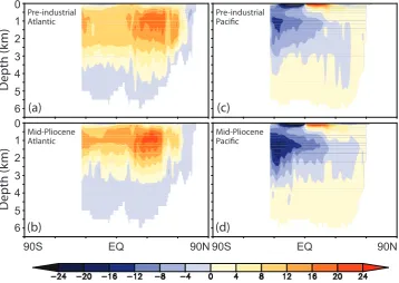
Earlier studies have pointed to an enhanced AMOC to ac-count for reconstructions of relatively warm mid-Pliocene sea surface temperatures in the North Atlantic (Dowsett et al., 1992; Raymo et al., 1996; Ravelo et al., 2000; Hodell et al., 2006; Dowsett et al., 2009, 2010). However, in our study the simulated AMOC is similar to that of the pre-industrial, with a maximum overturning stream function only 1.6 Sv stronger in the mid-Pliocene. More importantly, the return flow of NADW occurs at a slightly shallower depth in the mid-Pliocene experiment (Fig. 8).
0
3 2 1
4
5
6 0
3 2 1
4
5
6
90S EQ 90N90S EQ 90N
Atlantic
Atlantic
Pacific
Pacific
Pre-industrial Pre-industrial
Mid-Pliocene Mid-Pliocene
(a)
(d)
(c)
(b)
D
epth (k
m)
D
epth (k
m)
Fig. 8. Smoothed overturning stream function (Sv) (a) for industrial Atlantic Basin, (b) for mid-Pliocene Atlantic Basin, (c) for pre-industrial Pacific Basin and (d) for mid-Pliocene Pacific Basin.
6 Summary
In this paper, we describe pre-industrial and mid-Pliocene ex-periments simulated with the NorESM-L. Comparison of the simulation with observations demonstrates that the NorESM-L simulates a realistic pre-industrial climate. Compared to the pre-industrial simulation, the global mid-Pliocene surface temperature is 3.2◦C warmer. Warming occurs almost glob-ally, with stronger warming occurring in the high latitudes. In the mid-Pliocene experiment, global annual mean precip-itation increases by 0.2 mm day−1.
At the ocean surface, the simulated mid-Pliocene global mean SST is 2.0◦C warmer than the pre-industrial. More importantly, the warming exceeds 3◦C at the surface of the Greenland Sea, in the central North Atlantic, and in the Southern Ocean off the coast of East Antarctica. Salinity increases at the surface of the Atlantic, the Pacific and the Southern Ocean by 1 g kg−1, but decreases at the surface of
the Arctic and the Indian Oceans by 2 g kg−1.
Acknowledgements. This study was jointly supported by the Earth
System Modeling (ESM) project financed by Statoil, Norway, the National 973 Program of China (Grant No. 2010CB950102), and the National Natural Science Foundation of China (Grant No. 40902054). The NorESM development was supported by the Integrated Earth System Approach to Explore Natural Variability and Climate Sensitivity (EARTHCLIM) project, which is a nationally coordinated climate research project in Norway.
Edited by: D. Lunt
References
Adler, R. F., Huffman, G. J., Chang, A., Ferraro, R., Xie, P., Janowiak, J., Rudolf, B., Schneider, U., Curtis, S., Bolvin, D., Gruber, A., Susskind, J., and Arkin, P.: The Version 2 Global Precipitation Climatology Project (GPCP) Monthly Precipitation Analysis (1979–Present), J. Hydrometeor., 4, 1147–1167, 2003. Alterskjær, K., Kristj´ansson, J. E., and Seland, Ø.: Sensitivity
to deliberate sea salt seeding of marine clouds – observations and model simulations, Atmos. Chem. Phys., 12, 2795–2807, doi:10.5194/acp-12-2795-2012, 2012.
Assmann, K. M., Bentsen, M., Segschneider, J., and Heinze, C.: An isopycnic ocean carbon cycle model, Geosci. Model Dev., 3, 143–167, doi:10.5194/gmd-3-143-2010, 2010.
Bailey, D., Holland, M., Hunke, E., Lipscomb, B., Briegleb, B., Bitz, C., and Schramm, J.: Community Ice CodE (CICE) User’s Guide Version 4.0, available at: http://www.cesm.ucar. edu/models/cesm1.0/cice/doc/index.html, 2010.
Berger, A.: Long Term Variations of Daily Insolation and Quater-nary Climatic Changes, J. Atmos. Sci., 35, 2362–2367, 1978. Bitz, C. M. and Lipscomb, W. H.: An energy-conserving
thermody-namic sea ice model for climate study, J. Geophys. Res.-Oceans, 104, 15669–15677, 1999.
Bleck, R. and Smith, L. T.: A Wind-Driven Isopycnic Coordinate Model of the North and Equatorial Atlantic Ocean, 1, Model De-velopment and Supporting Experiments, J. Geophys. Res., 95, 3273–3285, 1990.
Chandler, M., Rind, D., and Thompson, R.: Joint investigations of the middle Pliocene climate II: GISS GCM Northern Hemisphere results, Global Planet. Change, 9, 197–219, 1994.
Dee, D. P., Uppala, S. M., Simmons, A. J., Berrisford, P., Poli, P., Kobayashi, S., Andrae, U., Balmaseda, M. A, Balsamo, G., Bauer, P., Bechtold, P., Beljaars, A. C. M., van de Berg, L., Bid-lot, J., Bormann, N., Delsol, C., Dragani, R., Fuentes, M., Geer, A. J., Haimberger, L., Healy, S. B., Hersbach, H., H´olm, E. V., Isaksen, L., K˚allberg, P., K¨ohler, M., Matricardi, M., McNally, A. P., Monge-Sanz, B. M., Morcrette, J. J., Park, B. K., Peubey, C., de Rosnay, P., Tavolato, C., Th´epaut, J. N., and Vitart, F.: The ERA-Interim reanalysis: configuration and performance of the data assimilation system, Q. J. Roy. Meteor. Soc., 137, 553– 597, doi:10.1002/qj.828, 2011.
Dowsett, H. J., Cronin, T. M., Poore, R. Z., Thompson, R. S., What-ley, R. C., and Wood, A. M.: Micropaleontological evidence for increased meridional heat transport in the North Atlantic Ocean during the Pliocene, Science, 258, 1133–1135, 1992.
Dowsett, H. J., Thompson, R., Barron, J., Cronin, T., Fleming, F., Ishman, S., Poore, R., Willard, D., and Holtz, T.: Joint Inves-tigations of the Middle Pliocene Climate I: PRISM Paleoenvi-ronmental Reconstructions, Global Planet. Change, 9, 169–195, 1994.
Dowsett, H. J., Barron, J., and Poore, R.: Middle Pliocene sea sur-face temperatures: a global reconstruction, Mar. Micropaleon-tol., 27, 13–25, 1996.
Dowsett, H. J., Barron, J. A., Poore, R. Z., Thompson, R. S., Cronin, T. M., Ishman, S. E., and Willard, D. A.: Middle Pliocene pale-oenvironmental reconstruction: PRISM2, US Geol. Surv., Open File Rep., 99–535, 1999.
Dowsett, H. J., Robinson, M. M., and Foley, K. M.: Pliocene three-dimensional global ocean temperature reconstruction, Clim. Past, 5, 769–783, doi:10.5194/cp-5-769-2009, 2009.
Dowsett, H. J., Robinson, M. M., Haywood, A. M., Salzmann, U., Hill, D., Sohl, L., Chandler, M., Williams, M., Foley, K., and Stoll, D.: The PRISM3D paleoenvironmental reconstruction, Stratigraphy 7, 123–139, 2010.
Dukowicz, J. K. and Baumgardner, J. R.: Incremental remapping as a transport/advection algorithm, J. Comput. Phys., 160, 318–335, 2000.
Eaton, B.: User’s Guide to the Community Atmosphere Model CAM-4.0, available at: http://www.cesm.ucar.edu/models/ ccsm4.0/cam/docs/users guide/ug.html, 2010.
Flato, G. M. and Hibler, W. D.: Ridging and strength in model-ing the thickness distribution of Arctic sea ice, J. Geophys. Res.-Oceans, 100, 18611–18626, 1995.
Hack, J. J., Boville, B. A., Briegleb, B. P., Kiehl, J. T., Rasch, P. J., and Williamson, D. L.: Description of the NCAR Com-munity Climate Model (CCM2), Technical Report NCAR/TN-382+STR, National Center for Atmospheric Research, 120 pp., 1993.
Hansen, J., Ruedy, R., Sato, M., and Lo, K.: Global surface temperature change, Rev. Geophys., 48, RG4004, doi:10.1029/2010RG000345, 2010.
Haywood, A. M. and Valdes, P. J.: Modelling Pliocene warmth: contribution of atmosphere, oceans and cryosphere, Earth Planet. Sci. Lett., 218, 363–377, 2004.
Haywood, A. M., Valdes, P. J., and Sellwood, B. W.: Global scale palaeoclimate reconstruction of the middle Pliocene climate
us-ing the UKMO GCM: initial results, Global Planet. Change, 25, 239–256, 2000.
Haywood, A. M., Dowsett, H. J., Otto-Bliesner, B., Chandler, M. A., Dolan, A. M., Hill, D. J., Lunt, D. J., Robinson, M. M., Rosenbloom, N., Salzmann, U., and Sohl, L. E.: Pliocene Model Intercomparison Project (PlioMIP): experimental design and boundary conditions (Experiment 1), Geosci. Model Dev., 3, 227–242, doi:10.5194/gmd-3-227-2010, 2010.
Haywood, A. M., Dowsett, H. J., Robinson, M. M., Stoll, D. K., Dolan, A. M., Lunt, D. J., Otto-Bliesner, B., and Chandler, M. A.: Pliocene Model Intercomparison Project (PlioMIP): experi-mental design and boundary conditions (Experiment 2), Geosci. Model Dev., 4, 571–577, doi:10.5194/gmd-4-571-2011, 2011. Hibler, W. D.: Modeling a variable thickness sea ice cover, Mon.
Weather Rev., 108, 1943–1973, 1980.
Hill, D. J., Haywood, A. M., Hindmarsh, R. C. A., and Valdes, P. J.: Characterising ice sheets during the mid Pliocene: evidence from data and models, in: Deep time perspectives on climate change: Marrying the signal from computer models and biological prox-ies, edited by: Williams, M., Haywood, A. M., Gregory, F. J., and Schmidt, D. N., the Micropalaeontological Society, Special Publications, the Geological Society, London, 517–538, 2007. Hodell, D. A. and Venz-Curtis, K. A.: Late Neogene history of
deepwater ventilation in the southern ocean, Geochem. Geophys. Geosyst., 7, Q09001, doi:10.1029/2005GC001211, 2006. Holtslag, A. A. M. and Boville, B. A.: Local versus nonlocal
boundary-layer diffusion in a global climate model, J. Climate, 6, 1825–1842, 1993.
Hunke, E. C. and Dukowicz, J. K.: An elastic-viscous-plastic model for sea ice dynamics, J. Phys.Oceanogr., 27, 1849–1867, 1997. Hunke, E. C. and Lipscomb, W. H.: CICE: the Los Alamos Sea
Ice Model Documentation and Software User’s Manual Version 4.1. LA-CC-06-012, available at: http://oceans11.lanl.gov/trac/ CICE, 2010.
Jansen, E., Overpeck, J., Briffa, K. R., Duplessy, J.-C., Joos, F., Masson-Delmotte, V., Olago, D., Otto-Bliesner, B., Peltier, W. R., Rahmstorf, S., Ramesh, R., Raynaud, D., Rind, D., Solom-ina, O., Villalba, R., and Zhang, D.: Palaeoclimate, in: Cli-mate Change 2007: The Physical Science Basis. Contribution of Working Group I to the Fourth Assessment Report of the In-tergovernmental Panel on Climate Change, edited by: Solomon, S., Qin, D., Manning, M., Chen, Z., Marquis, M., Averyt, K. B., Tignor, M., and Miller, H. L., Cambridge University Press, Cambridge, United Kingdom and New York, NY, USA, 2007. Jiang, D., Wang, H., Ding, Z., Lang, X., and Drange, H.:
Mod-eling the middle Pliocene climate with a global atmospheric general circulation model, J. Geophys. Res., 110, D14107, doi:10.1029/2004JD005639, 2005.
Kiehl, J. T., Hack, J. J., Bonan, G. B., Boville, B. B., Williamson, D. L., and Rasch, P. J.: The National Center for Atmospheric Research Community Climate Model: CCM3, J. Climate, 11, 1131–1149, 1998.
Kluzek, E.: CESM Research Tools: CLM4 in CESM1.0.3 user’s guide documentation, available at: http://www.cesm.ucar.edu/ models/cesm1.0/clm/models/lnd/clm/doc/UsersGuide/book1. html, 2011.
Lipscomb, W. H.: Remapping the thickness distribution in sea ice models, J. Geophys. Res.-Oceans, 106, 13989–14000, 2001. Lipscomb, W. H. and Hunke E. C.: Modeling sea ice transport using
incremental remapping, Mon. Weather Rev., 132, 1341–1354, 2004.
Lipscomb, W. H., Hunke, E. C., Maslowski, W., and Jakacki, J.: Improving ridging schemes for highresolution sea ice models. J. Geophys. Res.-Oceans, 112, C03S91, doi:10.1029/2005JC003355, 2007.
Lunt, D. J., Haywood, A. M., Foster, G., and Stone, E. J.: The Arctic cryosphere in the mid-pliocene and the future, Phil. Trans. R. Soc. A, 367, 49–67, 2009.
Meehl, G. A., Stocker, T. F., Collins, W. D., Friedlingstein, P., Gaye, A. T., Gregory, J. M., Kitoh, A., Knutti, R., Murphy, J. M., Noda, A., Raper, S. C. B., Watterson, I. G., Weaver, A. J., and Zhao, Z. C.: Global climate projections, in: Climate Change 2007: The Physical Science Basis, Contribution of Working Group I to the Fourth Assessment Report of the Intergovernmental Panel on Climate Change, edited by: Solomon, S., Qin, D., Manning, M., Chen, Z., Marquis, M., Averyt, K. B., Tignor, M., and Miller, H. L., Cambridge University Press, Cambridge, United Kingdom and New York, NY, USA, 770–772, 2007.
Neale, R. B., Richter, J. H., Conley, A. J., Park, S., Lauritzen, P. H., Gettelman, A., Williamson, D. L., Rasch, P. J., Vavrus, S. J., Taylor, M. A., Collins, W. D., Zhang, M., and Lin, S.: Descrip-tion of the NCAR Community Atmosphere Model (CAM 4.0), NCAR technical note, NCAR/TN-485+STR, 2010.
Oleson, K. W., Lawrence, D. M., Bonan, G. B., Flanner, M. G., Kluzek, E., Lawrence, P. J., Levis, S., Swenson S. C., Thornton, P., Dai, A., Decker, M., Dickinson, R., Feddema, J., Heald, C. L., Hoffman, F., Lamarque, J., Mahowald, N., Niu, G., Qian, T., Randerson, J., Running, S., Sakaguchi, K., Slater, A., St¨ockli, R., Wang, A., Yang, Z., Zeng, X., and Zeng, X.: Technical De-scription of version 4.0 of the Community Land Model (CLM), NCAR technical note, NCAR/TN-478+STR, 2010.
Rasch, P. J. and Kristj´ansson, J. E.: A comparison of the CCM3 model climate using diagnosed and predicted condensate param-eterizations, J. Climate, 11, 1587–1614, 1998.
Ravelo, A. V. and Andreasen, D. H.: Enhanced circulation during a warm period, Geophys. Res. Lett., 27, 1001–1004, 2000. Raymo, M. E., Grant, B., Horowitz, M., and Rau, G. H.:
Mid-Pliocene warmth: stronger greenhouse and stronger conveyor, Mar. Micropaleontol., 27, 313–326, 1996.
Raymond, D. J. and Blyth, A. M.: A stochastic mixing model for non-precipitating cumulus clouds, J. Atmos. Sci., 43, 2708– 2718, 1986.
Raymond, D. J. and Blyth, A. M.: Extension of the stochastic mix-ing model to cumulonimbus clouds, J. Atmos. Sci., 49, 1968– 1983, 1992.
Richter, J. H. and Rasch, P. J., Effects of convective momentum transport on the atmospheric circulation in the community atmo-sphere model, version 3, J. Climate, 21, 1487–1499, 2008. Rosenbloom, N.: Biome4 conversion to LSM, available
at: https://wiki.ucar.edu/display/paleo/Biome4+conversion+to+ LSM, 2009.
Rosenbloom, N., Shields, C., Brady, E., Yeager, S., and Levis, S.: CCSM3 for Paleoclimate Applications, 2010.
Rothrock, D. A.: The energetics of the plastic deformation of pack ice by ridging, J. Geophys. Res., 80, 4514–4519, 1975. Salzmann, U., Haywood, A. M., Lunt, D. J., Valdes, P. J., and Hill,
D. J.: A new global biome reconstruction and data-model com-parison for the Middle Pliocene, Global Eco. Biogeogr., 17, 432– 447, 2008.
Seland, Ø., Iversen, T., Kirkev˚ag, A., and Storelvmo, T.: Aerosol-climate interactions in the CAM-Oslo atmospheric GCM and in-vestigation of associated basic shortcomings, Tellus, 60A, 459– 491, 2008.
Simmons, A. J. and Str¨ufing R.: An energy and angular-momentum conserving finite-difference scheme, hybrid coordinates and medium-range weather prediction, Technical Report ECMWF Report No. 28, European Centre for Medium–Range Weather Forecasts, Reading, UK, 68 pp., 1981.
Slingo, J. M.: The development and verification of a cloud predic-tion scheme for the ECMWF model, Q. J. R. Meteorol. Soc., 113, 899–927, 1987.
Sloan, L. C., Crowley, T. J., and Pollard, D.: Modeling of middle Pliocene climate with the NCAR GENESIS general circulation model, Mar. Micropaleontol., 27, 51–61, 1996.
Sohl, L. E., Chandler, M. A., Schmunk, R. B., Mankoff, K., Jonas, J. A., Foley, K. M., and Dowsett, H. J.: PRISM3/GISS topographic reconstruction, US Geol. Surv. Data Series 419, 6 pp., 2009. Thorndike, A. S., Rothrock, D. A., Maykut, G. A., and Colony, R.:
The thickness distribution of sea ice, J. Geophys. Res., 80, 4501– 4513, 1975.
Vertenstein, M., Craig, T., Middleton, A., Feddema, D., and Fischer, C.: CESM1.0.3 User’s Guide, available at: http://www.cesm. ucar.edu/models/cesm1.0/cesm/cesm doc/book1.html, 2010. Yan, Q., Zhang, Z., Wang, H., Jiang, D., and Zheng, W.: Simulation
of sea surface temperature changes in the Middle Pliocene warm period and comparison with reconstructions, Chinese Sci. Bull., 56, 890–899, 2011.
Zeng, X., Zhao, M., and Dickinson, R. E.: Intercomparison of bulk aerodynamic algorithms for the computation of sea surface fluxes using the TOGA COARE and TAO data, J. Climate, 11, 2628– 2644, 1998.