A two-dimensional mathematical model of non-linear dual-sorption of percutaneous drug absorption

Open Access

Research

A two-dimensional mathematical model of non-linear dual-sorption

of percutaneous drug absorption

K George*

Address: 1_{School of Information Systems, Computing and Mathematics; Department of mathematical Sciences, Brunel University, Uxbridge,} Middlesex, , UB8 3PH, UK, 2_{Aditi College, University of Delhi, Bawana, Delhi, 110039, India and} 3_{Civil and Computational Engineering Centre,} School of Engineering, Singleton Park, Swansea, SA2 8PP Wales, UK

Email: K George* - [email protected] * Corresponding author

Abstract

Background: Certain drugs, for example scopolamine and timolol, show non-linear kinetic

behavior during permeation process. This non-linear kinetic behavior is due to two mechanisms; the first mechanism being a simple dissolution producing mobile and freely diffusible molecules and the second being an adsorption process producing non-mobile molecules that do not participate in the diffusion process. When such a drug is applied on the skin surface, the concentration of the drug accumulated in the skin and the amount of the drug eliminated into the blood vessel depend on the value of a parameter, C, the donor concentration. The present paper studies the effect of the parameter value, C, when the region of the contact of the skin with drug, is a line segment on the skin surface. To confirm that dual-sorption process gives an explanation to non-linear kinetic behavior, the characteristic features that are used in one-dimensional models are (1) prolongation of half-life if the plot of flux versus time are straight lines soon after the vehicle removal, (2) the decrease in half-life with increase in donor concentration. This paper introduces another feature as a characteristic to confirm that dual-sorption model gives an explanation to the non-linear kinetic behavior of the drug. This new feature is "the prolongation of half-life is not a necessary feature if the plots of drug flux versus time is a non-linear curve, soon after the vehicle removal".

Methods: From biological point of view, a drug absorption model is said to be nonlinear if the

sorption isotherm is non-linear. When a model is non-linear the relationship between lag-time and donor concentration is non-linear and the lag time decreases with increase in donor concentration. A two-dimensional dual-sorption model is developed for percutaneous absorption of a drug, which shows non-linear kinetic behavior in the permeation process. This model may be used when the diffusion of the drug in the direction parallel to the skin surface must be examined, as well as in the direction into the skin, examined in one-dimensional models. The dual-sorption model is an initial/ boundary value problem which consists of (1) one non-linear, two-dimensional, second-order parabolic equation, (2) boundary conditions, (3) one initial condition. Note that, the number of boundary conditions are, six and four, respectively, if the permeation process under consideration is, during the application of the vehicle and during the removal of the vehicle. Adopting the approach of method of lines, the initial/boundary value problem is transformed into an initial-value problem, which consists of (1) a system of non-linear ordinary differential equations, (2) one initial condition. The system of linear ordinary differential equations contains time-dependent non-homogeneous terms, if the permeation process under consideration is, during the application of

Published: 03 July 2005

BioMedical Engineering OnLine 2005, 4:40 doi:10.1186/1475-925X-4-40

Received: 06 December 2004 Accepted: 03 July 2005

This article is available from: http://www.biomedical-engineering-online.com/content/4/1/40

© 2005 George; licensee BioMed Central Ltd.

the vehicle. To solve this initial-value problem, an eight-stage sequential algorithm which is second-order accurate, and requires only tri-diagonal solvers, is developed.

Results: Simulation of the numerical methods described is carried out with various values of the

parameter C. The illustrations are given in the form of figures. The concentration profiles are viewed as parabolas along the mesh lines parallel to x-axis or y-axis. The flow rates in different subregions of the skin-region are studied. The shapes of the concentration profiles are examined before and after the steady-state concentration is reached. The concentration reaches steady-state when the flux reaches the steady state. The plots of flux versus time and cumulative amount of drug eliminated into the receptor cell versus time are given.

Conclusion: Based on the various values of the parameter, C, conclusions are drawn about (1)

flow rate of the drug in different regions of the skin, (2) shape of the concentration profiles, (3) the time required to reach the steady-state value of the concentration, (4) concentration of the drug in different regions of the skin, when steady-state value of the concentration is reached, (5) the time required to reach the state value of the flux, (6) time required to reach the steady-state value of the concentration of the drug, (7) half-life of the concentration of the drug and (8) lag-time.

A comparison, between this two-dimensional model and the one-dimensional non-linear dual-sorption model that exists in the literature, is done based on (1) the shape of the concentration profiles at various time levels, (2) the time required to reach the steady-state value of the concentration, (3) lag-time and (4) half-life.

Background

A non-linear model takes into account the property of the skin to sorb and bind substances during the process of permeation in addition to the ordinary dissolution. Such a non-linear model can be used to explain the disparity between the steady-state diffusivity of the drug in the skin and the unsteady-state value computed from transient (time-lag) permeation experiments, see [1]. A non-linear dual-sorption model of percutaneous drug absorption is described in [2]. Another mathematical model of percuta-neous drug absorption and its exact solution is described in [3]. In [4], the non-linear percutaneous permeation

kinetics of timolol is studied in vitro with human cadaver

skin. A model for a suspension with a finite dissolution rate is solved numerically in [5]. All these non-linear mod-els are one-dimensional and the region of contact of the

skin with the drug, is a single point, say x = 0, where x

measures the distance into the skin.

To the authors' knowledge, no two-dimensional non-lin-ear mathematical model of percutaneous drug absorption exists in the literature, where the region of contact is a line

segment, say x = 0, 0 ≤y ≤L_c. The purpose of this paper is

(1) to model the above situation mathematically (2) to obtain an efficient numerical method which can use a large time step compared to spacial discretization step; and also handles discontinuities between initial and boundary conditions in the mathematical model.

Methods

(a) Concentration before the steady state is reached (Concentration during the application of the vehicle)

Let the drug be applied as an ointment on the

skin-sur-face, say, {(0, y) : 0 ≤y ≤L_c}, at time t = 0. The

two-dimen-sional model developed in [6] takes into account the drug kinetics in the skin where the ointment is not directly applied. The one-dimensional non-linear dual-sorption model given in [2] postulates the total concentration of

the drug, C_T, in the skin is composed of two parts, (1) the

mobile solute concentration CD, which is due to the

mechanism of simple dissolution and is expressed as C_D =

K_DC, in which K_D is skin/receptor cell partition coefficient

and C is donor-cell concentration, (2) the immobile

sol-ute concentration C_I, which is due to the adsorption

proc-ess, and is expressed as , in which

is Langmuir's saturation constant and b is Langmuir's

affinity constant. Hence the total concentration CT, in the

skin is given by

CT = CD + CI.

Based on [6] and [2], to describe the drug kinetics at any

time t > 0, a two-dimensional non-linear dual-sorption

model is developed. Let the thickness (distance between the skin-surface and skin-capillary boundary) of the skin

be L_s. Assuming that skin is an isotropic medium, that is,

the diffusivity κ, is the same in the x and y directions, the

drug concentration C_D = C_D(x, y, t) in the skin is governed by

where L_s, L_d, L_u and L_c are positive real numbers. Note that,

(1) is non-singular as b > 0, > 0 and C_D ≥ 0. Following

[2], the concentration along the skin-receptor cell bound-ary may be considered to have the value zero. Assuming

that the donor-cell concentration at the uppermost

epider-mis {(0, y, t) : 0 ≤y ≤L_c, t > 0} is maintained at the value

C, the boundary conditions for the model are given by

C_D (0, y, t) = K_DC, 0 ≤y ≤L_c, t > 0, (2b)

C_D (L_s, y, t) = 0, -L_d ≤y ≤L_u, t > 0, (2f)

Assuming that there is no drug in the skin before the application, the initial distribution associated with the PDE is

CD(x, y, 0) = 0,0 ≤ × ≤Ls, -Ld ≤y ≤Lu (3)

The flux J = J(t), through the skin to the receptor site, per

unit area, is given by

The cumulative amount of drug eliminated into the

recep-tor cell per unit area at time τ(see [2]) is

The initial/boundary-value problem given by (1) to (3) is named as "problem (PA)".

(b) Concentration after the steady state is reached (Concentration after the vehicle removal)

Let T_s denote the time at which the steady-state is reached

by the problem (PA). Suppose that at time t = T_s, the

vehi-cle is removed instantaneously from the skin. Then (1) remains unchanged, but the initial conditions and bound-ary conditions changes and consequently, (2a) to (2c) dis-appear from the mathematical model, leaving the PDE's

C_D (L_s, y, t) = 0, -L_d ≤y ≤L_u, t > T_s (7d)

The initial distribution associated with PDE (6) is

C_D = C_D (x, y, T_s), 0 ≤x ≤L_s, -L_d ≤y ≤L_u, (8)

where C_D (x, y, T_s) is computed by solving problem (PA).

The initial/ boundary-value problem given by (6) to (8) is named as "problem (PB)".

Numerical methods

The approach to be adopted in obtaining a numerical solution, is the method of lines in which the initial/ boundary-value problem to be solved is transformed into

a first-order initial-value problem. At any time t > 0, the

region associated with the skin is given by R_s = {(x, y) : 0 ≤

x ≤L_s, - L_d ≤y ≤L_u}. The region of the contact R_c, of the

drug and the skin surface is defined as R_c = {(0, y) : 0 ≤y ≤

Lc}. Superimpose on Rs a rectangular grid with mesh

lengths, h > 0 and H > 0, respectively, in the x and y

direc-tions. Let k > 0 be a constant time step. Let N be a positive

integer, and h = 1/(N + 1). Also it is assumed that L_c = Q_cH,

L_u = Q_uH, L_d = Q_dH, where Q_c, Q_u and Q_d are positive inte-gers. The grid points are given by (x_l, y_m, t_j); x_l = lh, l = 0(1)(N + 1), y_m = mH, m = -Q_d(1)Q_u and t_j= jk, j = 0, 1, 2, ...s, ...etc. with sk = T_s. The values t_j represent the time-levels

for the problems (PA) and (PB) for j ≤s and j ≥s

respec-tively. The finite-difference solution which approximates

the solution C_D (x, y, t) of the two-dimensional parabolic

equation (1), is sought at each mesh point (x_l, y_m, t_j) in the

region [R_s- R_c - {(L_s, y), -L_d ≤y ≤L_u}] × t > 0. Note that, for

∂

∂ = + +

 

 _ ∂_∂ + ∂ ∂ 



 _

−

C t

bC bC

C x

C y

D I

D

D D

κ 1

1 2 1

1 2

2 2

2 *

( ) , ( )

0

0< <x Ls,−Ld < <y L Lu, u>L tc, >0,

C_I*

∂

∂ = − ≤ < >

C

x y t L y t

D

d

( , , )0 0, 0, 0, (2a)

∂

∂ = < ≤ >

C

x y t L y L t

D

c u

( , , )0 0, , 0, ( )2c

∂

∂ − = ≤ ≤ >

C

y x L t x L t

D

d s

( , , ) 0 0, , 0, (2d)

∂

∂ = ≤ ≤ >

C

y x L t x L t

D

u s

( , , ) 0 0, , 0, (2e)

J t C

x L y t dy D

L L

s d

u

( )= − ∂ ( , , ) ( )

∂ −

∫

κ 4

Ae Ae J x L t C

x L y t y t

s _L D

L s

d u

= = = = − ∂

∂

−

∫

∫

∫

( )τ τ ( )d κ τ ( , , )d d ( )5

0 0

∂

∂ = + +

 

 _ ∂_∂ + ∂ ∂ 



 _

−

C t

bC

bC

C

x

C

y

D I

D

D D

κ 1

1 2 6

1 2

2 2

2 *

( ) , ( )

0

0< <x Ls,−Ld < <y L tu, >Ts,

∂

∂ = − ≤ ≤ >

C

x y t L y L t T

D

d u s

( , , )0 0, , , (7a)

∂

∂ − = ≤ ≤ >

C

y x L t x L t T

D

d s s

( , , ) 0 0, , , (7b)

∂

∂ = ≤ ≤ >

C

y x L t x L t T

D

u s s

the initial-value problem (PB), R_c = Φ (the empty set). For the problem (PA), the differential equation (1), subject to the boundary conditions (2a) to (2f), is discretized at all grid points in the region [R_s - R_c -{(L_s, y), -L_d ≤y ≤L_u}] × [0

≤t ≤T_s]. For the problem (PB), the differential equation

(6), subject to the boundary conditions (7a) to (7d), is

discretized at all grid points in the region [Rs -{(Ls, y), -Ld

≤y ≤L_u}] × [t > T_s]. For notational simplicity, denote

Discretization for problem (PA)

At any time-level t = t_j, or , the {(Q_d + Q_u + 1)

(N + 1) - (Q_c + 1)} elements will be ordered in rows

par-allel to the x-axis and in vector form, and will be denoted

by C_D(t) and Q(t), where Q(t) is due to the boundary

con-dition (2b). For W = C_D and Q, and = or ,

denote

In the above notation n takes the value 0 if m ≠ 0(1)Q_c and

takes the value 1 otherwise. The vector C_D(t) is a vector of

unknowns and the vector Q(t) is given by

All other are zero. In the following discretizations,

(x_l, y_m), p_l,m, q_l,m and C_Dl,m, respectively, denote (x_l, y_m, t_j),

, and . At any time-level t = tj, the

differen-tial equation (1) can be discretized as

If and are respectively, suitable

approximations to C_Dxx;l;m and C_Dyy;l;m, the above

discreti-zation can be written as

At an interior grid point (x_l, y_m), and

are given by

If (xl, ym) is a boundary point, using the boundary

condi-tions (2a) to (2f), and are given by

where

A₁ = 0, B₁ = 2, if l = 0, m = -Q_d(1)(-1), (Q_c + 1)(1)Q_u,

A₁ = 0, B₁ = 1, if l = 1, m = 0(1)Q_c,

A1 = 1, B1 = 1, if l = 1(1)N - 1, m = -Qd(1)Qu,

A₁ = 1, B₁ = 0, if l = N, m = -Q_d(1)Q_u,

A₂ = 0, B₂ = 2, if l = 0(1)N, m = -Q_d,

A₂ = 2, B₂ = 0, if l = 0(1)N, m = Q_u,

A2 = 1, B2 = 1, if l = 0, m = (-Qd + 1)(1)(-2), (Qc + 2)(1)(Qu

- 1),

A₂ = 1, B₂ = 0, if l = 0, m = -1

A₂ = 0, B₂ = 1, if l = 0, m = (Q_c + 1).

System of ordinary differential equations

Combining the discretizations (9) together with

expres-sions for and given by (10) and (11)

respectively, a system of ordinary differential equations is formed as

where

C C x y t C C

x x y t

C C

Dl m j

D l m j Dx l m

j D

l m j

Dy l m

j D , ; , ; , ( , , ), ( , , ), = =∂ ∂ =∂

∂yy x y t etc

p C bC

bC p

l m j

D I D ( , , ),... , ( ) ( ) * = + +    _ − κ 1 1 2 1

and _{ll m}j I Dl m j bC bC , * , ( ) . = + +         − κ 1 1 2 1

C_{Dl m}j _, q_{l m}j_,

w_{l m}j_, C_{Dl m}j _, q_{l m}j_,

q_{l m}j_,

q

K C p

h

l m Q

K C p

H l m

l m j

D l m j

c

D l m j , , , ( ) , ( ) , ( ) , = = = = 2 2

1 0 1

0

if and

if and == − +

            1 1 0 , , , Q_c otherwise.

q_{l m}j_,

p_{l m}j_, q_{l m}j_, C_{Dl m}j _,

d

dt(CDl m, )=pl m,

(

)

1 2

2 h δx l mc,

1 2

2 H δy l mc,

d dt C

p

h C

p

H C q

Dl m l m x Dl m l m y Dl m l m

( , )= ,₂ δ2 , + ,₂δ2 , + , .

( )

δx2CDl m, δy2CDl m,

δ δ

x Dl m Dl m Dl m Dl m

y Dl m Dl m Dl m D

C C C C

C C C C

2 1 1 2 1 2 2 , , , , , , , , = − + = − + − +

− ll m, +1.

( )

δx2CDl m, δy2CDl m,

δ δ

x Dl m Dl m Dl m Dl m

y Dl m Dl m D

C A C C B C

C A C C

2

1 1 1 1

2 2 1 2 2 , , , , , , , = − + = − − +

− ll m, +B C2 Dl m, +1.

( )

δx2CDl m, δy2CDl m,

d

The value of m in Ed and Fd is -Qd, and that in Eu and Fu is

Q_c + 1. The abbreviations m1, m2, ... etc. represent m + 1,

m + 2, ... etc. For m ≠ 0, 1, 2, ...Q_c, E_m and F_m are square

matrices of order N + 1 and are given by

For m = 0, 1, 2, ..., Q_c, E_m and F_m are square matrices of

order N and are given by

For the values of m = -1, Q_c + 1, and m = 0, Q_c, the matrices

G_m are of orders (N + 1) × N and N × (N + 1), respectively,

and are given by

For the values of m = 0, 1, ..., Q_c, m ≠ 0, 1, 2, ...Q_c, the

matrices O_m are the zero matrices of orders N and N + 1

respectively. The matrices O_d and O_c are zero matrices of

orders (N + 1) × N and N × (N + 1), respectively.

Recurrence relation and its implementation via sequential algorithm

In [7], an eight stage sequential algorithm is described to solve two space linear parabolic equations. In [2], a sequential algorithm of two tridiagonal solvers is described to solve one-space non-linear dual-sorption model. To the author's knowledge, there is no sequential algorithm in the literature to solve the two-dimensional non-linear parabolic equation (1). The aim of this section is to develop an eight-stage sequential algorithm of tridi-agonal solvers, to solve the system of non-linear ordinary differential equations given by (12), which gives the solu-tion of two-space non-linear parabolic equasolu-tion (1). The main idea used is, to rewrite the system of equations (12) in such a way that, the numerical techniques described in [7] and [2] can be extended to two-space non-linear equa-tions. To achieve this, we proceed as follows.

Let Q(t) = R(t) + S(t), where the elements of the vectors

R(t) and S(t) are, respectively, denoted by and ,

and are defined by

Note that the vector, R(t), is the contribution of C_Dxx to the

vector Q(t). The vector, S(t), is the contribution of C_Dyy to

the vector Q(t). The system of non-linear ordinary

differ-ential equations given by (12) can be written as

It is known (see [2,8]) that the system of ordinary differ-ential equations given by (12), subject to the initial con-dition (3), satisfies the recurrence relation

where D* = diag{d/dt}. The exponential term in the

recur-rence relation (16) will be approximated by its (2, 0) Padé approximant to give

which, following pre-multiplication, gives

E h

E O O O E O O O E

F H

F O O O F O O O F

E =           =           1 1 2 2 d c u d u d

, c ;

==             = − − −

E O O O O

O E

E O

F

F F O

F

m m m d

m m

d

m m d

m

1 2 1

1

1

1

2 2

… …

, d −− −             = − − − 2 2 1 1

1 1 1

0 0 1

0 1

F Fm

F F G

E

O E O O

O O E

E m c c … , c Q Q c c

Q Q Q

c O c c c

F

G F F O

F F F

F F G

            = − − −   , c

0 0 0

1 1 1

2 2 2 …             =               = , , E

O E O O

O E

E F

G

d m m Q

m m Q Q u u c u u 1 1 … ₊₊ − − −               1

1 1 1

2 2

2 2

F F O

F F F

F F

m m Q

m m m

Q Q u u u … . E p p

p p p

p p

F m

m m

m m m

N m N m m = − − −             2 2 2 2 0 0

1 1 1

, , , , , , , , ==            ( ) p p p m m N m 0 1 0 0 0 0 0 0 13 , , , . E p p

p p p

p p

F m

m m

m m m

N m N m m = − − −             = 2 2 2 1 1

2 2 2

, , , , , , , , pp p p m m N m 1 2 0 0 0 0 0 0 14 , , , . … … …            ( ) G p p p m m m

N m _{N N}

=             + ×

0 0 0 0

0 0 0

0 0 0

0 0 0

1 2 1 … … … … , , , _{( )}

,for mm Q

p p p c m m N m = − +            1 1

0 0 0 0 0

0 0 0 0

0 0 0 0

0 0 0 0

1 2 and … … … … , , ,                    

 N N× +

c Q

( )

, .

1

for m=0 and

αl m j

, βl m j ,

α

β

l m

j l m

j l m j q , , , , , =_ 

for 1 and = 0(1)Q ,

otherwise.

and

c

l= m

0

==_ 

q_{l m}j_, , ,

for 1, Q + 1 and = 0,

otherwise. c

l =− m

0

d

dtCD( )t =( ( )E tCD( )t +R( )) ( ( )t + F tCD( )t +S( ))t ( )15

CD(t+k)=(ekD )CD( ),t ( )

∗

16

C_D(t+k)=I−kD + kD C_D( ),t



 

∗ 1 ∗

2

1

( )2

I−kD + kD t k t

 



 + =

∗ 1 ∗

2( ) 17

2 _{C C}

Using the split form (15), and following [7] and [2], a four-stage sequential algorithm is developed to obtain

, which is an approximation to C_D(t + k) in (17). It is

given by

(I - r₁kE) Z = C_D(t) + r₁kR(t), (18a) (I - r2kE) V = Z + r2kR(t), (18b)

(I - r₁kF) Z = V + r₁kS(t), (18c)

(I - r₂kF) (t + k) = Z + r₂kS (t). (18d)

where (see [8])

Another solution, , which is an approximation to C_D(t

+ k) in (17), is obtained by interchanging the matrices E

and F; and the vectors R and S; in (18a) to (18d). It is

given by

(I - r₁kF) Z = C_D(t) + r₁kS(t), (18e) (I - r₂kF) V = Z + r₂kS(t), (18f) (I - r₁kE) Z = V + r₁kR(t), (18g)

(I - r₂kE) (t + k) = Z+ r₂kR (t). (18h)

Note that the approximations, and , given by

(18d) and (18h), are first-order accurate in time and their linear combination defined by

is second order accurate in time. The eight-stage

algo-rithm, defined by (18a) to (18i) is, L0 stable and uses only

tridiagonal solver.

Initial/boundary value problem (PB)

The "problem (PB)" is modelled by the equations (6) to

(8). At any time-level t = t_j, j ≥s, , the (Q_d + Q_u + 1)

× (N + 1) elements, will be ordered in rows parallel to the

x-axis and in vector form, and will be denoted as C_D(t),

with

At a grid point x_l, y_m, the required discretization is

For l ≠ 0, m ≠ (-Qd + 1) (1) (Qu - 1); and

are given by (10) and for l = 0, m = (-Q_d + 1)(1)(Q_u - 1),

and

Combining the discretizations given by (19), a system of differential equations is formed as

in which

In the above matrices, the value of m is -Qd and m1 = m +

1, m2 = m + 2,... The matrices E_i and F_i, i = -Q_d(1)Q_u, are

square matrices of order N +1, and are given by (13).

Pro-ceeding as in problem (PA), the eight-stage algorithm to solve the system of differential equations (20), subject to the initial conditions (8), is

(I - r₁kE) Z = C_D(t), (21a) (I - r₂kE) V = Z , (21b) (I - r1kF) Z = V, (21c)

(I - r2kF) (t + k) = Z, (21d)

(I - r₁kF) Z = C_D(t), (21e) (I - r2kF) V = Z, (21f)

(I - r₁kE) Z = V, (21g)

CD∗∗

CD∗∗

r₁=r₂ =1₂+i

C_D+

C_D+

CD∗∗ CD+

C_D(t+k)=1 C_D t+k C_D , ( )

2( ( ) + ( + )) 18i

∗∗ + _{t k}

C_{Dl m}j _,

CD( )t C ,C ,..,C ;C ,C ,..,C ;

C D Q

j

D Q j

D j

D j

D j

DQ j

DQ

d d c

c

=  − − + −

+

1 1 0 1

1

1 2

0 1

j

DQ j

DQ j

Dm j

D m j

D m j

D N m j

C C

C C C C

c u

, ,.., ,

, ,..,

, , ,

+ _

=  where

 ,m= −Qd( )1Qu.

d dt C

p h

C p

H C

Dl m l m x Dl m m y Dl m

( _, )= , _, + , _, , ( )

2 2

2

2 ₁₉

δ l δ

δx2CDl m, δy2CDl m,

δ_x2C_{D m0,} = −2C_{D m0,} +2C_{D m1,}

δy2CD m0, =CD m0, −1−2CD m0, +CD m0, +1.

d

dtCD( )t =(E+F)CD( )t (20)

E h

E E

E F

H

F F

F F F

F m

m

Q

m m

m m m

u

= 

    



    

= −

−

−

1 1

2 2

2

2

2

1

2

1 1 1

,

Q Q_u 2FQ_u



    



    

,

(I - r2kE) (t + k) = Z, (21h)

Note that the sequential algorithm defined by (21a) to (21i) is obtained from the equations (18a) to (18i),

replacing the vectors R(t) and S(t), by the zero vector of

length (Q_d + Q_u+ 1) × (N + 1). This shows the efficiency of

the splitting of the vector Q(t), and the eight-stage

algo-rithm developed in problem (PA).

Stability Analysis

The stability analysis of two-stage sequential algorithm for the solution of one-space non-linear second-order para-bolic equation is described in [2]. The stability analysis of four-stage sequential algorithm for the solution of two-space second-order parabolic equation is described in [7]. In this section, following [7] and [2], it is to prove that the eight-stage sequential algorithms described by (18a) to

(18i) and (21a) to (21i) are L0 stable.

The amplification matrix R*(k(E + F)) of the method

defined by (18a) to (18d) is given by

neglecting the higher order terms O (-k3_).

Hence the symbol R*(-z), of the method defined by (18a)

to (18d), to evaluate (t + k) is given by

Similarly the symbol R+_{(--z), of the method defined by}

(18e) to (18h), to evaluate (t + k) is given by

In (22) and (23), z = -kλwhere λis an eigen value of the

matrix E + F. Hence using (22) and (23) the symbol, S(-z),

of the method (18i) is

The method is L₀ stable if

| S(-z) | ≤ 1 (24)

S(-z) → 0, as z →∞

• Proof of (24):- Applying Brauer's theorem, it can be

shown that all the eigen values λof the matrix E + F are

negative. Hence, z = kλ > 0.

• Proof of

(25):-From (24) and (25), it is concluded that the numerical

method defined by (18a) to (18i) is L₀ stable. Similarly

the numerical method defined by (21a) to (21i) is L0

sta-ble. Since the method is L₀ stable, the discontinuities

around y = 0 and y = L_c are not propagated.

Results and discussion

In order to examine the behavior of the recurrence rela-tions (18a) to (18i) and (21a) to (21i), a series of five numerical experiments, similar to those described in [2], are carried out for two space dimensions. In these experi-ments the parameter-values used are those used in [2]. For

the experiments numbered n = 1, 2, 3, 4, and 5, the

param-eter C was given the values 4.1, 19.5, 43.1, 51.4 and 64.0

respectively. The rest of the parameter values are given by

L_s = 0.004 cm, L_d = 0.0320 cm, Lc = 0.128 cm, L_u = 0.160 cm,

k = 0.1 h, H = 0.0004, κ= 0.0000018 cm2_{/h, = 5.0 mg/}

ml, K_D = 1.1, h = 0.0002, N = 19, Q_c = 320, Q_u = 400, Q_d =

80, b = 0.5599 ml/mg.

It was assumed in all numerical experiments that the drug was applied until steady-state concentration profile is

reached. Let denotes the time in hours, at which the

concentration profiles for the nth _{(n = 1, 2, 3, 4 and 5)}

experiment reaches the steady-state. Suppose that at time

t = , the vehicle is removed instantaneously from the

skin. The pattern of the concentration profile is observed for fifty hours more, after the vehicle is removed at the

steady-state. For the nth _{(n = 1(1)5) experiment, the values}

of C_D are computed (1) using the sequential algorithm

(18a) to (18i), in the time interval 0 <t ≤ , (2) using

the sequential algorithm (21a) to (21i), in the time

inter-val <t ≤ + 50. Following [2], for the value of n =

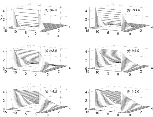
1 (C = 4.4), the profiles of concentration C_D at t = 0.5. 1.0,

2.0, 3.0, 4.5 and 6.0 are given in figure 1. In figure 2, the

profiles of concentration C_D are given at t = 24.0, 26.0,

CD+

CD(t+k)=1 CD t+k CD ( )

2( ( ) + ( + )). 21i

∗∗ + _{t k}

R k E F I r kE I r kE I r kF I r kF

I k E F k

∗ _{+ =}

_[

_]

− + +

( ( )) ( )( )( )( )

( )

1 2 1 2

1 2

2

2 1 2(E+F) ,

 

 _

−

C_D∗∗

R z

z z

∗ _{− =}

+ +

( ) 1 . ( )

1

22

2

2

C_D+

R z

z z

+_{(− =) , ( )}

+ +

1

1

23

2

2

S z R z R z

z z (− =) ( (− +) (− ))=

+ +

∗ +

1 2

1

1 ₂2

z k z

z

S z z

z

= − > ⇒ + + > ⇒

+ + < ⇒ − ≤

λ 0 1 1 1

1

1 1

2

2 2

2

| ( ) | .

S z

z

S z z

z

z

z z

(− =) ( ) , .

+ + = + + ⇒ − → → ∞

1

1

0

2

2

2

2

1 1 1 1

2

as

C_I*

T_s( )n

T_s( )n

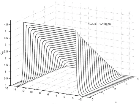
28.0, 30.0, 32.0 and 34.0. In figure 3 the profile of

con-centration C_D, are given at time t = = 128.7, the time

at which concentration, C_D, reaches the steady state for the

first experiment. In figures 1, 2 and 3, the concentration

profiles are viewed as parabolas along mesh lines x = xl, l

= 0(1) N. The figures 1 and 2 show the flow rate in

differ-ent subregions of the skin region R_s, before the

concentra-tion reaches the steady state. Figure 3 shows the shape of the concentration profile when the concentration reaches steady-state.

In figure 4 and figure 5, for the value of C = 4.4, the

con-centration profiles at t = 0.5 and 3.0 are viewed as

parab-olas along the mesh lines y = y_m, m = -Q_d(1)Q_u. Figure 4

and figure 5 show the change in shape of the parabolas in the region away from the region of contact of drug and

skin. In figure 6, corresponding to the value of C = 4.4, the

concentration profiles at t = = 128.7 are shown along

the mesh lines y = y_m, m = Q_c(1)Q_u. The figure 6 shows the

importance of two-dimensional modelling.

Corresponding to each value of n = 1(1)5, the

concentra-tion profiles at t = are given in figures 7, 8, 9, 10 and

11, respectively. The above figures show the effect of the

value of C on the steady-state concentration C_D in

differ-ent regions of R_s.

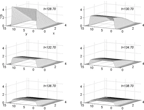
In figure 12, the concentration profiles for the value of C

= 4.4 are given at t = 128.7, 130.7, 132.7, 134.7, 136.7,

and 138.7. This graph show the rate of decreasing of the

Concentration profiles for C = 4.4, viewed as parabolas along mesh lines x = xl, l = 0(1)N; t = 0.5, 1.0, 2.0, 3.0, 4.5, 6.0

Figure 1

Concentration profiles for C = 4.4, viewed as parabolas along mesh lines x = xl, l = 0(1)N; t = 0.5, 1.0, 2.0, 3.0, 4.5, 6.0.

T_s( )1

T_s( )1

concentration in different regions of R_s after the removal of the vehicle.

The A_e versus time and J versus time profiles are monitored

for the time interval 0 ≤t ≤ + 50 in each experiment.

The values J and A_e are computed at each time step using

the trape-zoidal rule to approximate the integrals in (4)

and (5). Thus, to second-order accuracy, for j = 1, 2, 3,...

etc,

where

and

In literature see [2], the drug absorption experiments are monitored for a large time interval. Hence it is desirable to use a numerical method which gives acceptable results with larger time steps compared to spacial discretization.

Since the numerical method used in this section are L₀

sta-ble, it is expected to give accurate results when a large time

Concentration profiles for C = 4.4, viewed as parabolas along mesh lines x = xl, l = 0(1)N; t = 24.0, 26.0, 28.0, 30.0, 32.0, 34.0

Figure 2

Concentration profiles for C = 4.4, viewed as parabolas along mesh lines x = xl, l = 0(1)N; t = 24.0, 26.0, 28.0, 30.0, 32.0, 34.0.

T_s( )n

J t H

h A A

j N

j

N j

( )= −κ ( ₋ − ), ( )

4 1 4 26

A_nj C_{Dn m}j C C n N N

m Q

Q

Dn Q j

Dn Q j

d u

d u

= + + = −

=− + −

−

∑

2 1

1 1

, , , with , ;

Ae t_j J t_i J t_j i

j

( )= k ( ) ( ) . ( )

2 2 ₁ 27

1

+ 



step is used. Note that the conclusions obtained from all

the five experiments are independent of the time step k. As

an illustration, with k = 0.1 and k = 0.01, J versus time

pro-files are monitored for the first experiment (C = 4.4) and

are given in figure 15. The time required to reach the

steady-state value of the flux with k = 0.1 and k = 0.01

respectively are t = 128.7 and t = 130.37. When the

numer-ical computation is done with k = 0.01, the difference in

flux during the time interval [128.7 130.37] is 10-10_,

which is negligible. It is also noted that even if the drug is

Concentration profiles for C = 4.4, viewed as parabolas along

mesh lines at x = x_l, l = 0(1)N; t = 128.7

Figure 3

Concentration profiles for C = 4.4, viewed as parabolas along mesh lines at x = xl, l = 0(1)N; t = 128.7.

Concentration profiles for C = 4.4, viewed as parabolas along

mesh lines at y = y_m, m = -Q_d(1)Q_u; t = 0.5

Figure 4

Concentration profiles for C = 4.4, viewed as parabolas along mesh lines at y = ym, m = -Qd(1)Qu; t = 0.5.

0 1

2 3

4

−2 0 2 4 6 8 10 12 14 16 0 0.5 1 1.5 2 2.5 3 3.5 4 4.5

x C=4.4, t=128.70

y

C

D

0 1

2 3

4

−2 0 2 4 6 8 10 12 14 16

0 0.5 1 1.5 2 2.5 3 3.5 4 4.5

x C=4.4, t=0.5

y

C

D

Concentration profiles for C = 4.4, viewed as parabolas along

mesh lines at y = y_m, m = -Q_d(1)Q_u; t = 3.0

Figure 5

Concentration profiles for C = 4.4, viewed as parabolas along mesh lines at y = ym, m = -Qd(1)Qu; t = 3.0.

Concentration profiles for C = 4.4, viewed as parabolas along

mesh lines at y = ym, m = 0(1)Qc; t = 128.7

Figure 6

Concentration profiles for C = 4.4, viewed as parabolas along mesh lines at y = y_m, m = 0(1)Q_c; t = 128.7.

0 1

2 3

4

−2 0 2 4 6 8 10 12 14 16

0 0.5 1 1.5 2 2.5 3 3.5 4 4.5

x C=4.4, t=3.0

y

C

D

0 1

2 3

4

0 2 4 6 8 10 12 14

0 0.5 1 1.5 2 2.5 3 3.5 4 4.5 5

x C=4.4, t=128.70

y

C

removed at t = 130.37 instead of t = 128.7, the conclusions drawn in next section remain valid.

Conclusion

Conclusion is presented in five parts.

Part 1:- Conclusions based on concentration profiles till steady-state concentration, C_D, is reached

Concentration profiles at various time levels are examined until steady state is reached. Graphically these concentration profiles are represented as parabolas along

mesh lines x = x_l, l = 0(1) N or parabolas along mesh lines

Concentration profiles for C = 4.4, when steady-state is

reached Figure 7

Concentration profiles for C = 4.4, when steady-state is reached.

Concentration profiles for C = 19.5, when steady-state is

reached Figure 8

Concentration profiles for C = 19.5, when steady-state is reached.

0 1

2 3

4

−2 0 2 4 6 8 10 12 14 16

0 0.5 1 1.5 2 2.5 3 3.5 4 4.5 5

x n=1, C=4.4, T(1)

s=128.70

y

C

D

0 1

2 3

4

−2 0 2 4 6 8 10 12 14 16

0 5 10 15 20 25

x n=2, C=19.5, T(2)

s=104.1

y

C

D

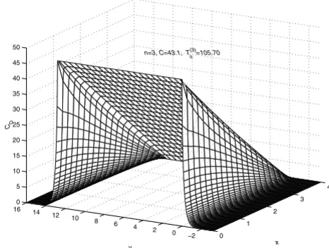
Concentration profiles for C = 43.1, when steady-state is

reached Figure 9

Concentration profiles for C = 43.1, when steady-state is reached.

Concentration profiles for C = 51.4, when steady-state is

reached Figure 10

Concentration profiles for C = 51.4, when steady-state is reached.

0 1

2 3

4

−2 0 2 4 6 8 10 12 14 16

0 5 10 15 20 25 30 35 40 45 50

x n=3, C=43.1, T(3)_s=105.70

y

C

D

0 1

2 3

4

−2 0 2 4 6 8 10 12 14 16

0 10 20 30 40 50 60

x n=4, C=51.4, T(4)

s=125.30

y

C

y = y_m, m = -Q_d(1)Q_u. Divide the region of skin, R_s, into two

mutually exclusive regions R₁ and R₂ as follows.

R₁ = R_c × L_s and R₂ = R_s - R₁.

The following conclusions are drawn based on drug kinet-ics in the regions R1, R2 and Rs.

(1) In figure 1 the concentration profiles are viewed as

parabolas along mesh lines x = x_l, l = 0(1)N. Consider the

flow rate of concentration of the drug in the region R₁.

From the subplots (a) to (c) of figure 1, it is concluded that during the initial time levels, flow rate towards the skin surface is larger than flow rate towards the skin-cap-illary boundary. Later-on time levels (from subplots (c) to (f) of figure 1), flow rate towards the skin-capillary boundary becomes larger than flow rate near to the skin surface.

(2) In figure 2 the concentration profiles are viewed as parabolas along mesh

lines x = xl, l = 0(1)N.

From figure 1 and figure 2 it is concluded that in the

region R₂, the flow rate near to the skin surface is larger

than flow rate towards the skin-capillary boundary.

(3) Consider the flow rate in the whole region R_s. From

figure 1 and figure 2 it is concluded that, during the initial

time levels, flow rate in the region R1 is larger than the

flow rate in the region R₂. But later-on time levels, flow

rate in the region R₂ becomes larger than the flow rate in

the region R₁, leading to a steady-state concentration

file as given in figure 3. In figure 3 the concentration

pro-files are viewed as parabolas along mesh lines x = x_l, l =

0(1)N.

(4) At any time level t = t_j, consider the concentration of

the drug along the mesh line x = x_l, l = 0(1)N. From figure

1, 2 and 3, it is concluded that the concentration of the drug at a mesh point (x_l, y_m, t_j) ∈R₁, m = 0(1)Q_c is larger

than the concentration of the drug at a mesh point (xl, ym,

t_j) ∈R₂, m ≠ 0(1)Q_c.

(5) In figure 4 and figure 5, the concentration profiles are

viewed as parabolas along mesh lines y = y_m, m =

-Q_d(1)Q_u. From figure 4 it is concluded that, during the

ini-tial time-levels, the shape of the parabolas in the whole

region R_s retains the same shape as the shape of the

con-centration profiles given in page 97 of [2]. If a one-dimen-sional model of drug absorption was sufficient, the following results are expected from [2].

• When steady-state concentration reaches, the shape of

the concentration profiles viewed along the mesh lines y =

y_m, m = -Q_d(1)Q_u is same as the shape of the parabolas

given in page 97 of [2].

• When steady-state concentration reaches, concentration

profiles along the mesh lines y = y_m, m = 0(1)Q_c are straight

lines.

Contrary to this result, the following results are obtained from two-dimensional modelling.

5.1 From figure 4 and figure 5 it is concluded that, as time

increases, the parabolas in the region R₂ have a convex

shape, whereas the parabolas given in page 97 of [2] have a concave shape.

5.2 The concentration profiles along the mesh lines, y =

y_m, m = 5(1) Q_c - 5 are straight lines. These straight lines are

shown in figure 6.

5.3 The concentration profiles along the mesh lines, y =

y_m, m = 0, 1, 2, 3, 4, Q_c - 4, Q_c - 3, Q_c - 2, Q_c - 1 and Q_c are not straight lines, but they have the shape as shown in fig-ure 6.

Even though the illustration of figures is done only for

one experiment (with n = 1, C = 4.4), that is only for the

first experiment, the conclusions drawn are true for all

other experiments (that is, for all values of C).

Concentration profiles for C = 64.0, when steady-state is

reached Figure 11

Concentration profiles for C = 64.0, when steady-state is reached.

0 1

2 3

4

−2 0 0 2 4 6 8 10 12 14 16

0 10 20 30 40 50 60 70 80

x n=5, C=64, T(5)

s=115.60

y

C

Part 2:-Conclusions based on concentration profiles when steady-state value of concentration is reached

The steady-state concentration profiles for all the five experiments are given in figure 7, figure 8, figure 9, figure 10 and figure 11. From these steady-state concentration profiles, the following conclusions are drawn.

(1) As the value of C increases, the concentration at any

point (x_l, y_m, t_j) increases.

(2) As the value of C increases, the difference between the

concentrations of the drug at mesh points (x_l, y_m, t_j) ∈R₁,

m = 0(1)Q_c and (x_l, y_m, t_j) ∈R₂, m ≠ 0(1)Qc increases.

(3) As the value of C increases, the difference between the

concentrations of the drug at mesh points (x₀, y_m, t_j) and

(x_N-1, y_m, t_j) increases for m = -Q_d(1)Q_c. This increase in

dif-ference is more prominent in the region R1 than in the

region R₂.

Part 3:-Conclusions based on concentration profiles after the removal of the vehicle when steady-state is reached

The vehicle is removed when the concentration reaches steady-state. The concentration profiles are examined for ten more hours, after the vehicle-removal, in an interval of two hours. In figure 12, these concentration profiles are

given for n = 1 (C = 4.4), at time levels t = = 128.7, t =

130.7, t = 132.7, t = 134.7, t = 136.7, and 138.7. From

fig-ure 12 the following conclusions are made.

Concentration profiles for C = 4.4 viewed as parabolas along mesh lines x = xl, l = 0(1)N; t = 128.7, 130.7, 132.7, 134.7, 136.7,

138.7 Figure 12

Concentration profiles for C = 4.4 viewed as parabolas along mesh lines x = xl, l = 0(1)N; t = 128.7, 130.7, 132.7, 134.7, 136.7, 138.7.

(1) After the removal of the vehicle, rate of decrease in the

region R₁ is larger than that in R₂.

(2) After the removal of the vehicle, rate of decrease near to the region of skin-surface is larger than that near to region of skin-capillary boundary. Even though the

illus-tration of figures is done only for one experiment (with n

= 1, C = 4.4), that is only for the first experiment, the

con-clusions drawn are true for all other experiments also.

Part 4:-Conclusions based on figure 13 (flux versus time) and figure 14 (Ae versus time)

The graphs of J versus time and Ae versus time for the time

interval 0 ≤ t ≤ ( + 50) are shown in figure 13. The

fol-lowing conclusions are drawn based on figure 13.

(1) As the value of C increases, the steady-state value of

flux increases.

(2) As the value of C increases half-life decreases, during

the time levels, soon after the vehicle-removal. There is no prolongation of half-life during later-on time, as stated in [2]. It is evident from figure 13 that, the plots of a drug

flux versus time is a non-linear curve, soon after the vehicle

removal. Hence, in experimental studies even when the prolongation of half-life is not seen, the nonlinearity of

drug flux versus time can be introduced as a characteristic

to confirm that dual-sorption model gives an explanation to non-linear kinetic behavior of the drug.

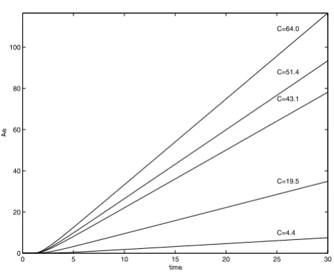
The graphs of Ae versus time for the time interval 0 ≤t ≤

+ 50 are shown in figure 14.

J versus time profiles for various values of C

Figure 13

J versus time profiles for various values of C.

Ae versus time profiles for various values of C

Figure 14

Ae versus time profiles for various values of C.

0 20 40 60 80 100 120 140 160

0 0.5 1 1.5 2 2.5 3 3.5 4 4.5

n=1, C=4.4, T(1)_s=128.70 n=2, C=19.5, T(2)_s=104.10 n=3, C=43.1, T(3)

s=105.70 n=4, C=51.4, T(4)_s=125.30 n=5, C=64.0, T(5)

s=115.60

time

J

0 5 10 15 20 25 30

0 20 40 60 80 100

time

Ae

C=4.4 C=19.5 C=43.1 C=51.4 C=64.0

J versus time profiles for C = 4.4 with k = 0.1 and k = 0.01 Figure 15

J versus time profiles for C = 4.4 with k = 0.1 and k = 0.01.

:

C 4.4 19.5 43.1 51.4 64.0

T_L1 3.44 2.29 1.99 1.93 1.84

TL2 3.67 2.52 2.16 2.11 2.04

0 20 40 60 80 100 120 140 160 180

0 0.05 0.1 0.15 0.2 0.25

time

J

K=0.1 K=0.01

T_s( )n

Publish with BioMed Central and every scientist can read your work free of charge "BioMed Central will be the most significant development for disseminating the results of biomedical researc h in our lifetime."

Sir Paul Nurse, Cancer Research UK

Your research papers will be:

available free of charge to the entire biomedical community

peer reviewed and published immediately upon acceptance

cited in PubMed and archived on PubMed Central

yours — you keep the copyright

Submit your manuscript here:

http://www.biomedcentral.com/info/publishing_adv.asp

BioMedcentral

(3) As the value of C increases, at any time level t = t_j, the

value of Ae(t) increases.

(4) As the value of C increases, time decreases. The

lag-time is computed as t-intercepts of the linear portion of

graphs of Ae versus time. For various values of C, the

lag-times are compared with the lag-lag-times given in [2]. Let TL1

denotes the lag-times quoted in [2] as a result of

one-dimensional modelling of drug-absorption and T_L2

denotes the lag-times obtained as a result of

two-dimen-sional modelling. Table 1 gives the values of T_L1 and T_L2,

corresponding to each value of C.

From Table 1 it is concluded that, for a particular value of

C, the lag-time obtained as a result of two-dimensional

modelling is greater than the lag-time obtained as a result of one-dimensional modelling. For a linear model, lag

time is independent of donor concentration C. The linear

model corresponding to (1) is obtained by substituting

= 0. Its lag time is computed as 1.56 which is greater than 1.44, the lag-time obtained from the

one-dimen-sional linear model (substitute = 0 in (8) of [2]).

It is an established fact that the drug permeation profiles of a nonlinear model is different from that of a linear model, as a non-linear model assumes that the drug molecules are either dissolved or immobile inside the skin. In this article it is shown that the drug permeation described by the two-dimensional non-linear model is different from one-dimensional non-linear model, as the two-dimensional model takes into account the drug kinetics at the site distant from the area where the oint-ment is directly applied.

Acknowledgements

The author thanks DST, Government of India, for the award of a BOY-SCAST fellowship.

References

1. Chandrasekaran SK, Michaels AS, Campbell PS, Shaw JE: Scopo-lamine permeation through human skin in vito. Am Inst Chem Eng J 1976, 22:828-832.

2. Gumel AB, Kubota K, Twizell EH: A sequential algorithm for the nonlinear dual-sorption model of percutaneous drug absorption. Mathematical Biosciences 1998, 152:87-103.

3. Kubota K, Ishizaki T: A calculation of percutaneous drug

absorption-I. Theoretical. Comput Biol Med 1986, 16:7-19. 4. Kubota K, Koyama E, Twizell EH: Dual sorption model for the

nonlinear percutaneous permeation kinetics of timolol. J Pharmaceutical Sciences 1993, 82:1205-1208.

5. Kubota K, Twizell EH, Maibach HI: Drug release from a suspen-sion with a finite dissolution rate: Theory and its application to a betamethasone 17-valerate patch. J Pharmaceutical Sciences

1994, 83:1593-1599.

6. George K, Kubota K, Twizell EH: A two-dimensional mathemat-ical model of percutaneous drug absorption. BioMedical Engi-neering OnLine 2004, 3:18.

7. Gumel AB: Parellel and sequential algorithms for

second-order parabolic equations with applications. In PhD thesis

Brunel University; 1993.

8. Twizell EH: Numerical Methods, with applications in the Biomedical Sciences Ellis Horwood, Chichester and Wiley, Newyork; 1998.

C*_I