www.geosci-model-dev.net/7/2223/2014/ doi:10.5194/gmd-7-2223-2014
© Author(s) 2014. CC Attribution 3.0 License.
FLEXINVERT: an atmospheric Bayesian inversion framework for
determining surface fluxes of trace species using an optimized grid
R. L. Thompson and A. Stohl
Norwegian Institute for Air Research, Kjeller, Norway
Correspondence to: R. L. Thompson ([email protected])
Received: 20 May 2014 – Published in Geosci. Model Dev. Discuss.: 10 June 2014 Revised: 21 August 2014 – Accepted: 31 August 2014 – Published: 30 September 2014
Abstract. We present a new modular Bayesian inversion framework, called FLEXINVERT, for estimating the surface fluxes of atmospheric trace species. FLEXINVERT can be applied to determine the spatio-temporal flux distribution of any species for which the atmospheric loss (if any) can be described as a linear process and can be used on continental to regional and even local scales with little or no modifica-tion. The relationship between changes in atmospheric mix-ing ratios and fluxes (the so-called source–receptor relation-ship) is described by a Lagrangian Particle Dispersion Model (LPDM) run in a backwards-in-time mode. In this study, we use FLEXPART but any LPDM could be used. The frame-work determines the fluxes on a nested grid of variable res-olution, which is optimized based on the source–receptor re-lationships for the given observation network. Background mixing ratios are determined by coupling FLEXPART to the output of a global Eulerian model (or alternatively, from the observations themselves) and are also optionally optimized in the inversion. Spatial and temporal error correlations in the fluxes are taken into account using a simple model of ex-ponential decay with space and time and, additionally, the aggregation error from the variable grid is accounted for. To demonstrate the use of FLEXINVERT, we present one case study in which methane fluxes are estimated in Europe in 2011 and compare the results to those of an independent in-version ensemble.
1 Introduction
Observations of atmospheric mixing ratios (or concentra-tions) of trace species (gases or aerosols) contain information about their fluxes between land/ocean and the atmosphere.
Atmospheric inversions use this information formally in a statistical optimization to find spatio-temporal distributions of trace gas (or aerosol mass) fluxes (e.g. Tans et al., 1990). This can be done provided that there is a model of atmo-spheric transport relating changes in fluxes to changes in mixing ratios (or concentrations) – that is, the so-called source–receptor relationships (SRRs). Basically, two types of models are used: Eulerian models, in which atmospheric transport and chemistry are calculated relative to a fixed coor-dinate, or Lagrangian Particle Dispersion Models (LPDMs), in which diffusion and chemistry are calculated from the per-spective of air parcels transported by ambient winds.
forward model developments and these being implemented in the adjoint. A further disadvantage is that these systems are computationally demanding, as they require forward and adjoint model runs for every iteration until convergence.
LPDMs are self-adjoint, i.e. they can track the dispersion of virtual particles representing e.g. an atmospheric gas for-ward in time from its sources/sinks to receptors (i.e. mea-surement sites) or backwards in time from receptors to its sources/sinks using the identical model formulation (Stohl et al., 2003; Seibert and Frank, 2004; Flesch et al., 1995). The forward and backward calculations are equivalent but one direction can be much more computationally efficient than the other. For instance, if there are few receptors but many sources/sinks, the backwards mode is more efficient. This is the case, for instance, when particles are tracked backwards from a relatively small number of available atmospheric ob-servation sites (i.e. receptors), as in our demonstration case. This feature makes LPDMs very efficient for the purpose of atmospheric inversion and they have been previously used in numerous studies (e.g. Gerbig et al., 2003; Lauvaux et al., 2009; Stohl et al., 2010; Thompson et al., 2011; Keller et al., 2012; Brunner et al., 2012). Lagrangian models may be used on a global scale (e.g. Stohl et al., 2010), sub-continental scale (e.g. Gerbig et al., 2003) or on a regional scale of the or-der of a few hundred square kilometres (e.g. Lauvaux et al., 2009). Owing to their favourable treatment of atmospheric turbulence in the boundary layer, LPDMs can even be used down to scales of a few hundreds of metres (Flesch et al., 1995) and have been used for inferring source strengths for local sources (e.g. farmsteads and oil spills). A further ad-vantage of LPDMs is that they can be run backward ex-actly from a measurement site, unlike Eulerian models, in which site measurements are represented by the averaged value of the corresponding grid cell. By focusing on local or regional scales, fine resolution may be used without running into problems of too large a number of unknown variables (in this case the fluxes). Fine resolution is desirable as it reduces the model representation error, also known as aggregation er-ror (Kaminski et al., 2001; Trampert and Snieder, 1996) but it must be traded-off with the total number of flux variables to be determined, which is subject to computational constraints. Using LPDMs to solve the inverse problem, however, also has disadvantages. In LPDMs, virtual particles are typically followed backward in time only for the order of days to a few weeks, thus the influence of the atmospheric chemistry and transport and surface fluxes further back in time (the so-called background mixing ratio) must be taken into account separately. Although forward 3-D simulations in LPDMs are possible, in order to reproduce background signals, such as seasonal variability, simulations of months to years would be necessary and, therefore, computationally too expensive (Stohl et al., 2009). Alternatively, the background mixing ra-tio can be accounted for using either observara-tion- or model-based approaches. Observation-model-based approaches use some filtering method (either statistical or based on meteorological
criteria) to identify observations representative of the back-ground, i.e. air not (or only minimally) influenced by fluxes during the time of the backwards calculations (e.g. Stohl et al., 2009; Manning et al., 2011). However, the background is strongly influenced by meteorology – e.g. air transported from higher latitudes or altitudes may have significantly dif-ferent mixing ratios compared to air transported from lower latitudes or altitudes even if in both cases no emissions oc-cur during the backward calculation. This makes the determi-nation of an observation-based background difficult. Model-based approaches involve coupling the back-trajectories at their point of termination to the mixing ratios determined from a global model.
One approach is to run the LPDM on a regional domain and couple this to a global model at the domain boundary. This approach was adopted by Rödenbeck et al. (2009), who use a two-step method to first solve for the fluxes on a coarse grid using an Eulerian model and to calculate the background mixing ratios at the receptors, and second to perform the inversion at regional scale on a finer grid using an LPDM. A similar approach was developed by Rigby et al. (2011) but using a one-step method. A drawback of both these ap-proaches, however, is that only the coarse-resolution Eule-rian model is used to calculate the background mixing ratios at the receptors and, thus, is more susceptible to transport er-rors. We use a different approach and couple the LPDM, run on a global scale, to an Eulerian model at the time boundary, such as done by Koyama et al. (2011). This approach uti-lizes the more accurate transport of the LPDM to calculate the background at the receptors.
In this paper, we present a new framework, called FLEX-INVERT, for optimizing fluxes by employing an LPDM that can be coupled to mixing ratio fields from a global (Eule-rian) model. This method may be used from large continental scales down to local scales and can be used for sparse as well as dense observation networks. In this method, the LPDM is used to transport air masses and, thus, the influence of fluxes, to each receptor. The fluxes inside the domain are optimized on a grid of variable resolution, where finer resolution is used in areas with a strong observation constraint, i.e. close to re-ceptors, and coarser resolution is used elsewhere. FLEXIN-VERT, as it is presented here, requires that the LPDM is run on a global domain, or at least that the domain is large enough so that trajectories do not exit the domain. In summary, the features of this method are:
– atmospheric transport (SRR) is calculated using a single model, i.e. the LPDM;
– the variable resolution grid means that fine resolution close to receptors minimizes model representation er-rors;
– background mixing ratios can be provided either by coupling to mixing ratio output from a global model or alternatively by using an observation-based method; – the background mixing ratios are optionally included in
the optimization;
– the influence of fluxes from outside the domain on the mixing ratios at the receptors is accounted for without having to solve for them explicitly, thereby reducing the dimensionality of the problem.
Variable grid resolution has been used in atmospheric in-versions previously such as in the studies of Manning et al. (2003), Stohl et al. (2010) and Wu et al. (2011). Our method for defining the variable grid is based on that of Stohl et al. (2010). However, we have also implemented a re-optimization of the fluxes at variable resolution back to the finest model resolution based on the method of Wu et al. (2011).
This paper is structured as follows: first we describe the inversion framework and the variable grid formulation and, second, we present an example using real observations of methane (CH4)dry-air mole fractions to optimize CH4 emis-sions in Europe.
2 Bayesian framework for linear inverse problems 2.1 Forward model
For cases where the atmospheric transport and chemistry are linear, the change in mixing ratio of a given atmospheric species can be related to its fluxes by a matrix operator. Fur-thermore, the absolute mixing ratio can be related to its fluxes plus the background mixing ratio, which together form the so-called state vector. This is shown in Eq. (1) whereymod(M×1) is a vector of the modelled mixing ratio atMpoints in time and space, x(N×1) is a vector of theN state variables dis-cretized in time and space, and H(M×N )is the transport op-erator:
ymod=Hx. (1)
For simplicity, we describe the case where the state vari-ables are optimized for only one time step, although the framework is able to optimize many time steps simultane-ously (for an overview of the variables and their dimensions see Tables 1 and 2). We construct the matrix H from three components of the atmospheric transport to each receptor: (1) transport of fluxes within a nested domain (i.e. within the global domain), Hnest, (2) transport of fluxes outside the nested domain, Hout, and (3) contribution of mixing ratios at
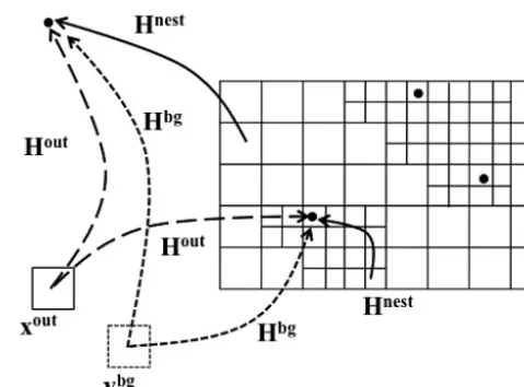
Figure 1. Schematic showing how the forward model is defined.
The black dots represent receptors, the solid boxes represent grid-ded fluxes and the dotted box represents gridgrid-ded mixing ratios from global model output. The arrows indicate transport to a receptor (which may be either inside or outside the nested domain): solid ar-rows show transport from fluxes within the nested domain, dashed arrows indicate transport from fluxes outside the nested domain, and the dotted arrows indicate transport of the mixing ratio at the point of back-trajectory termination. Each arrow can be thought of as an element (i.e. a partial derivative) in the transport matrix, Hnest,
Hout, and Hbg, respectively.
the time and location when the back-trajectories terminate, i.e. the initial mixing ratios, Hbg(see Fig. 1). Similarly,xis constructed from the fluxes inside the domain,fnest, fluxes outside the domain, fout (there are no common variables betweenfnest andfout so there is no double counting of fluxes), and initial mixing ratios taken from the output of a global model,ybg. (Note that here we refer to the contribu-tion to the observed mixing ratio from where the trajectories terminate as the initial mixing ratio and the contribution from the initial mixing ratio plus from the fluxes outside the do-main as the background mixing ratio – this is explained in Sect. 2.1.2). Equation (1) can thus be expanded to
ymod=Hnestfnest+Houtfout+Hbgybg. (2) 2.1.1 The source–receptor relationships (SRRs) The matrices Hnestand Houtare Jacobians in which each el-ement is a partial derivative of the change in mixing ratio at a given receptor with respect to the change in mass flux in a given grid cell and are built from the SRRs. In this study, we use the LPDM, FLEXPART (Stohl et al., 2005, 1998) to derive the SRRs, although any other LPDM capable of run-ning in backwards mode could also be used to construct these matrices.
Table 1. Overview of the variables used in this manuscript
Variable Dimension Description
ymod M×1 modelled atmospheric mixing ratios x N×1 state vector
H M×N complete atmospheric transport operator fnest K×1 fluxes inside the nested domain
Hnest M×K atmospheric transport operator for inside the nested domain fout P×1 fluxes outside the nested domain
Hout M×P atmospheric transport operator for outside the nested domain
ybg P×1 mixing ratios from the global model interpolated to the fine grid globally
Hbg M×P sensitivity to initial mixing ratios from the global model
0 W×K prolongation operator from the fine to the variable grid in the nested domain fnestvg W×1 fluxes inside the nested domain on the variable grid
Hnestvg M×W atmospheric transport operator for fluxes on the variable grid
Mcg M×R total background mixing ratios
0cg R×P prolongation operator from fine to coarse grid
0bg R×M prolongation operator for observation-based background mixing ratios acg R×1 background mixing ratio scalars
xb N×1 prior state vector of fluxes and background mixing ratio scalars σ W×1 prior flux error vector
B N×N prior error covariance matrix on the variable grid
Bfluxvg W×W prior error covariance matrix for the fluxes on the variable grid
Bflux K×K prior error covariance matrix for fluxes on the fine grid
R M×M observation error covariance matrix
C W×W spatial and temporal correlation matrix
CS W×W spatial correlation matrix
CT 1×1 temporal correlation matrix (trivial case when only one time step is used) A N×N posterior error covariance matrix
Aflux W×W posterior error covariance matrix for fluxes on the variable grid fnest∗ K×1 posterior fluxes optimized on the fine grid
Aflux∗ N×N posterior error covariance matrix for fluxes on the fine grid
P Q×K operator to select variables that violate the inequality constraint c Q a vector of inequality constraints
analysis data. Backwards and forwards calculations are prac-tically equivalent because the transport is time reversible (Seibert and Frank, 2004). For a tracer, which undergoes neg-ligible loss in the atmosphere on the timescale of the LPDM calculations, the SRR can be expressed for a receptor and a flux in a given spatio-temporal grid cell (i, n), as propor-tional to the average residence time ofJ back-trajectories in the grid cell under consideration:
∂y ∂xi,n
= 1 J
J X
j=1
1ti,j,n0
ρj,n
, (3)
whereρi,nis the air density in the grid cell and1ti,j,n0 is the residence time of trajectoryj in the spatio-temporal grid cell (i,n)(see Seibert and Frank, 2004). In Eq. (3), the SRR is in units of residence time×volume per unit mass, which is integrated over the height of the surface layer in FLEXPART to be comparable with the surface flux, which is given per unit area. Atmospheric loss processes, such as reaction with the hydroxyl radical, dry and wet deposition, or radioactive
decay, can be considered by including a transmission func-tion in the right-hand side of Eq. (3), which quantifies the loss. The SRRs for all receptors and fluxes inside the nested domain constitute the elements of Hnestwhile the SRRs for all receptors and fluxes outside the domain constitute the el-ements of Hout.
2.1.2 Initial mixing ratios
Table 2. Overview of the dimension notation and their values in the case study (test S1).
Dimension Description Value
M total number of observations 1602
N total number of state variables (12 time steps) 13 896
K number of fine resolution grid cells in one time step 2400
W number of variable resolution grid cells in one time step 1158
P number of grid cells in global domain in one time step 2700
R number of coarse grid cells for the background mixing ratio 144
∂y ∂yi
=ni
J. (4)
Again, loss processes can be considered by including a transmission function in the right-hand side of Eq. (4). The sensitivity to the mixing ratio in all P grid cells (over the global domain) and for allMobservations is represented by the matrix Hbg(M×P ) and the mixing ratios from the global model by the vectorybg(P×1), which has been interpolated to the resolution of the LPDM output. Thus, the initial mixing ratio at all receptors is Hbgybg.
The second alternative approximates the background mix-ing ratios from the observations themselves. In this case, the background mixing ratio is calculated in one step, i.e. there is no separate calculation of the initial mixing ratio and contribution from outside the nested domain. We have implemented a simple method involving selecting the lower quartile of the observations in a moving time window (e.g. 30 days) over the whole time series. This method was cho-sen as it is robust to the number of observations (i.e. it can be used for in situ as well as discrete measurements) al-though other more sophisticated background selection algo-rithms exist and could be used instead (e.g. Ruckstuhl et al., 2012; Giostra et al., 2011). The selected observations are the approximation for the contribution to the mixing ratio without any influence from fluxes in the nested domain – thus, the corresponding elements of the prior modelled mix-ing ratio, Hnestfnest, should be zero. However, this is not always the case, therefore, we also subtract the prior sim-ulated mixing ratio from the selected observations so that there is zero contribution from fluxes inside the domain in the background mixing ratio. To avoid overestimating the contribution from inside the domain and, hence, underesti-mating the background mixing ratio, we also select the lower quartile of the prior simulated mixing ratios in a moving time window. Lastly, we calculate a running average of the back-ground mixing ratios using a time window of 90 days, which is then linearly interpolated to the timestamp of the observa-tions. This is done for each receptor. Similar methods for the background calculation have been used previously for cases where no reliable global model estimate of the mixing ratio was available (e.g. Stohl et al., 2010).
2.2 Variable resolution grid
To reduce the number of variables in the inversion prob-lem we aggregate grid cells where there is little constraint from the atmospheric observations. In this way, we define a new vector of the fluxes to be optimized, fnest
vg , and trans-port matrix, Hnestvg , which are on a grid of variable resolution (vg=variable grid). The aggregation algorithm is based on time-averaged SRRs optionally convolved with the prior flux estimate. The variable grid is set up starting with a coarse grid, which is refined in a specified number of steps following the method of Stohl et al. (2009). For example, starting with a coarse resolution of 4◦×4◦the grid may be refined in two steps to resolutions of 2◦×2◦and 1◦×1◦. The refinement is made so that the flux sensitivity (optionally multiplied by the prior flux) in each grid cell at its final resolution (e.g. 1◦×1◦, 2◦×2◦and 4◦×4◦) is above a given threshold. It is also op-tional whether or not to make the grid refinement over water bodies and ice so that grid cells with a water/ice area of 99 % or more are not refined further, reflecting cases where the wa-ter/ice surface fluxes are either smaller, more homogeneous and/or more certain than the land surface fluxes. For deter-mining which grid cells are land/water/ice we use the In-ternational Geosphere Biosphere Programme land-cover data set (IGBP-DIS) (Belward et al., 1999).
To convert from the fine to the variable grid, we define a projection operator0(W×K) whereK is the number of grid cells in the nested domain at the original resolution andWis the number at variable resolution. Each row of0corresponds to a cell in the variable grid, and is a summation vector on the fine grid. The row vectorsλi of 0are orthogonal, thus λiλTj=0 fori6=j (since each fine grid cell can only belong to one variable grid cell). The flux vectorfnestand the matrix Hneston the variable grid can be found according to
fnestvg =0fnest and Hnestvg =Hnest0T, (5) where “T” indicates the matrix transpose. The fluxes infnest are weighted by the ratio of the area of fine grid to the vari-able grid into which it is aggregated. The forward model on the variable resolution grid can thus be written as
where εagg(M×1) is the model representation error from hav-ing reduced the resolution of the model (for a schematic for the forward model see Fig. 1). It is also known as the aggregation error and has been described by Trampert and Snieder (1996), Kaminski et al. (2001) and Thompson et al. (2011). We describe the calculation of the aggregation er-ror in Sect. 2.5.
2.3 Aggregation of the background mixing ratios The contribution of fluxes outside the domain to the change in mixing ratios at the receptor points (i.e. Houtfout)can be added to the initial mixing ratio (Hbgybg). The contribution to the modelled mixing ratio (i.e. ymod), which is not ac-counted for by the SRRs and fluxes inside the domain (i.e. the background mixing ratio), is then defined by a new ma-trix, Mcg(M×R), on a coarse grid (cg), which has rows cor-responding toMobservations and columns corresponding to
R grid cells or latitudinal bands. When the initial mixing ra-tio is calculated using the sensitivity matrix, Hbgand mixing ratio fields,ybgfrom a global Eulerian transport model, then Mcgis defined as
Mcg=
Hout◦Fout+Hbg◦Ybg0cgT, (7) where◦indicates the Hadamard matrix product, Fout(M×P )has
M rows of (fout)T, and Ybg(M×P ) has M rows of (ybg)T. The matrix 0cg(R×P ) is a projection operator from the Eu-lerian model resolution to a coarse resolution ofRgrid cells (note0cg6=0). Noteworthy, is that the matrix multiplication Hout◦Foutis made using the original resolution of the LPDM and fluxes and that the conversion to the coarse grid is per-formed only on the mixing ratios, thus avoiding an aggrega-tion error in this component. When the background is calcu-lated using the observations themselves, then Mcgis defined as
Mcg=diag(ybg)0Tbg, (8)
where0bg(R×M)is an operator to map the background mix-ing ratios to a matrix where the background for each mea-surement is allocated to one ofRlatitudinal bands. Note that the contribution from grid cells outside the domain is not explicitly included as it is assumed that this contribution is incorporated into the definition ofybg when it is calculated from the observations (see Sect. 2.1.2).
For both methods, the columns of Mcgcorrespond to the mixing ratios in each of theR coarse-grid cells (or latitudi-nal bands when using the observation-based method) such that the sum of each row gives the total background mixing ratio for each measurement (note that for the observation-based method there is only one non-zero entry in each row). The spatial distribution of the contribution to the background mixing ratio (dimensionR)is maintained as it is these con-tributions that are optimized in the inversion.
We then define a new transport operator H(M×N )by con-catenating the matrices Hnestvg and Mcg. Similarly, we define the state vectorx(N×1)by concatenatingfnestvg(W×1)(the flux variables inside the nested domain) and acg(R×1) (scalars of the mixing ratios in the columns of Mcg):
H=hHnestvg Mcg i
and x=hfnestvg acg i
. (9)
The prior value ofacg(i)(i=1 toR)is 1. After inversion, the optimized values ofacg determine the posterior back-ground mixing ratios.
2.4 Optimization of the fluxes and background mixing ratios
The uncertainty in the initial mixing ratios and in the con-tribution to the mixing ratio from fluxes outside the domain can be considerable. Therefore, we include this component in the optimization problem. The prior state vector for op-timization,xb, thus contains variables for the surface fluxes (on the variable-resolution grid) and variables for the opti-mization of the mixing ratios (on the coarse-resolution grid defined by0cg).
Based on Bayes’ theorem, the most probable solution for x is the one that minimizes the difference between the ob-served and modelled mixing ratios while also depending on the prior state variables,xb, and their uncertainties (for de-tails on Bayes’ theorem see e.g. Tarantola, 2005). Assum-ing that the uncertainties have a Gaussian probability density function (pdf) this can be described by the cost function
J (x)=1
2(x−xb)
TB−1(x−x b)
+1
2
Hx−yobsTR−1Hx−yobs, (10) where B(N×N ) is the prior flux error covariance matrix (see Sect. 2.5), R(M×M) is the observation error covariance ma-trix (see Sect. 2.6), andyobsis a vector of the observed mix-ing ratios. There exist a number of methods to find thexfor which Eq. (10) is at a minimum; we use the approach of find-ing the first derivative of Eq. (10) and solvfind-ing this forx. By rearrangement,xcan be found according to Eq. (11). Equa-tion (11) has a number of alternative formulaEqua-tions and the one we use is the most efficient when the number of obser-vations is smaller than the number of unknowns, since the size of the matrix to invert (HBHT+R) has dimensions of
M×M:
x=xb+BHT HBHT+R −1
yobs−Hxb
. (11)
The inverse of (HBHT+R) is found by Cholesky factor-ization (using the DPOTRF and DPOTRI routines from the LAPACK library). The corresponding posterior error covari-ance matrix, A(N×N ), is the inverse of the second derivative of the cost function,J:
2.5 Prior error covariance matrix
Errors in the prior flux estimates are correlated in space and time owing to correlations in the biogeochemistry model, up-scaling model, or anthropogenic emission inventory that was used to produce these estimates. Most often, there is little known about the true temporal and spatial error correlation patterns. Here we define the spatial error correlation for the fluxes as an exponential decay over distance, such that each element in the spatial correlation matrix CSis
cS(i,j )=exp
−dij kS
, (13)
wheredijis the distance between grid cellsiandjin a given time step and kS is the spatial correlation scale length on land or ocean (we assume that fluxes on land and ocean are not correlated with one another). The temporal error corre-lation matrix CTis described similarly using the time differ-ence between grid cells in different time steps. The full tem-poral and spatial correlation matrix C is given by the Kro-necker product: CT⊗CS. The error covariance matrix for the fluxes, Bfluxvg(W×W ), is the matrix product of correlation pat-tern, C, and the error covariance of the prior fluxes, σ σT, whereσ is a vector of the flux errors. We calculate the error on the flux in each grid cell (on the fine grid) as a fraction of the maximum value out of that grid cell and the eight sur-rounding ones. Finally, the Bfluxvg matrix is scaled so that the square root of its sum is consistent with a total error value assigned for the whole domain. This error estimate may be from e.g. comparisons of independent biogeochemistry mod-elled fluxes or flux inventories. The correlation matrix could be calculated for the fine grid and converted to the variable grid using the prolongation operator as0Bflux0T. However, we calculate Bfluxvg directly for the variable grid (dimensions
W×W ) as the multiplication step Bflux0T is very slow if
K is large and/or if there are many time steps. In addition, Bflux(K×K) is calculated for the fine grid for a single time step only, as it is needed in the calculation of the aggregation er-ror (see Sect. 2.6) and for the optimization of the posterior fluxes back to the fine grid (Sect. 2.8). We assume that the errors for the scalars of the background mixing ratios (i.e. acg)are uncorrelated and have a fixed prior value (e.g. 1 %). The error variance for these scalars is appended to Bflux
vg to give B(N×N ).
2.6 Aggregation error
The aggregation incurred by reducing the spatial resolution of the model can be calculated by projecting the loss of infor-mation in the state space into the observation space (Kamin-ski et al., 2001). The full aggregation error covariance matrix Eagg(M×M)is given by
Eagg=H0−B flux0T
−H
T, (14)
where0− is the projection of the loss of information in the variable grid compared to the fine grid. The matrix0−can be calculated simply from the row vectorsλi of the projection operator0, which are weighted by the square root of the row sum so as to have unit length:
0−=I− W X
i=1
λiλTi, (15)
where I is the identity matrix. AsλiλTi is a matrix of size P×P, whereP can be on the order of 10 000 to 100 000, it is not calculated directly but rather via H0−as follows:
H0−=H− W X
i=1
HλiλTi. (16)
2.7 Observation error covariance matrix
model and measurement representation errors:
σ2=σmeas2 +σtrans2 +σrepr2 . (17) Another assumption that is made is that the observed– modelled mixing ratio residuals have a Gaussian distribu-tion (Eq. 10 is based on this assumpdistribu-tion). Therefore, in cases where the distribution is highly skewed, observations corre-sponding to the tail of the distribution will have a strong in-fluence on the result of the inversion. FLEXINVERT does not include any component to deal with skewed distributions; however, the influence of observations in the tail of the dis-tribution may be reduced by increasing their uncertainty. For more details about dealing with skewed distributions we refer the reader to Stohl et al. (2009).
The observation error covariance matrix, R(M×M), is the sum of this diagonal matrix plus the aggregation error co-variance matrix, Eagg.
2.8 Optimization of the fluxes to fine resolution
The optimal solution of the fluxes, fnestvg ∗, is found for the variable grid according to Eq. (11) and the corresponding posterior error covariance matrix, A, is found according to Eq. (12). However, it is not possible to directly apply the in-verse of the projection operator to retrieve the optimal emis-sions at fine resolution since the operation from the variable to the fine resolution is ambiguous; there is insufficient in-formation to redefine the fluxes at fine resolution. To find the optimal emissions at fine resolution,fnest∗
(K×1), we use an adaptation of the method of Wu et al. (2011). This method in-volves a second Bayesian optimization step, which uses the prior information about the distribution of the fluxes within each grid cell on the variable resolution grid:
fnest∗=fnestb +Bfluxnaw0Tunit0Bflux0T+Aflux −1
fnestvg ∗−0fnestb , (18) (see Appendix A for the derivation of Eqs. 18 and 19). Since we only optimize the fluxes, i.e.fnest∗, the matrices Bfluxand Afluxrepresent only the parts of the error covariance matrices corresponding to flux errors. We have introduced a new er-ror covariance matrix, Bfluxnaw, which is the non-area-weighted (naw) version of Bflux, i.e. calculated using the flux errors not weighted by the ratio of the grid cell areas on the fine and coarse grid. Also, we have introduced 0unit, which is equivalent to0but with each row vector normalized by the row sum so that they have unit length. Our method departs from that of Wu et al. (2011) in that for the error in posterior state vector on the variable grid we use the error covariance of the posterior solution on the variable grid A, rather than a Dirac distribution. The inverse of (0Bflux0T+Aflux)is found by singular value decomposition (SVD) using the DGESDD routine from the LAPACK library. We find the posterior error
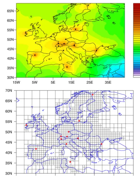
Figure 2. Total emission sensitivity for 2011 in units of
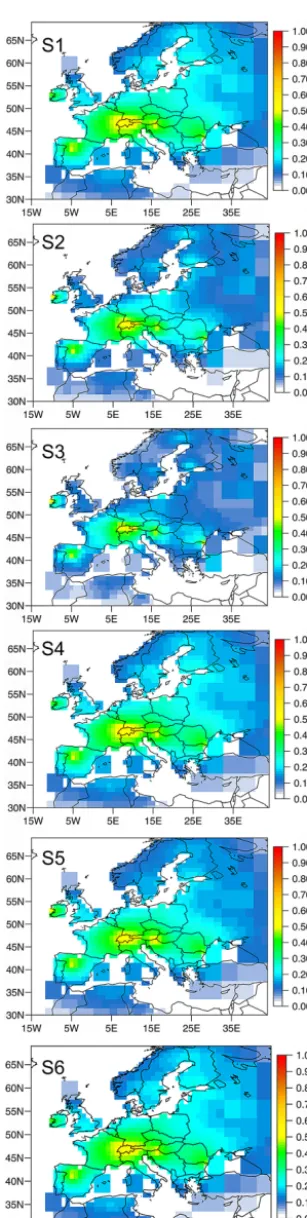
log(s m−3kg−1)calculated using FLEXPART and used to deter-mine the variable grid (note that for this no weighting is applied for the number of observations available from each site) (a) and the variable-resolution grid used in the inversion (b). The points indi-cate the positions of the observation sites.
covariance matrix Aflux(K×∗K)also for the fine-resolution fluxes according to
Aflux∗=Bflux-1naw +0unitT Aflux-10unit −1
. (19)
The inverse of the matrices Bfluxnaw, Aflux, and (Bflux-1naw + 0unitT Aflux-10unit)are also found by SVD, which can also be used for matrices that are non-positive definite. This opti-mization to the fine grid should be carefully evaluated if used. Alternatively, we also include a simple mapping back to the fine grid by distributing the flux in a coarse grid to the corre-sponding fine grid cells based on the prior relative flux dis-tribution at fine resolution.
2.9 Inequality constraints
Table 3. Atmospheric observation sites for CH4mole fraction used in the case study. The altitude is given in metres above sea level.
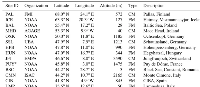
Site ID Organization Latitude Longitude Altitude (m) Type Description
PAL FMI 68.0◦N 24.1◦E 572 CM Pallas, Finland
ICE NOAA 63.3◦N 20.3◦W 127 FM Heimay, Vestmannaeyjar, Iceland BAL NOAA 55.4◦N 17.2◦E 28 FM Baltic Sea, Poland
MHD AGAGE 53.3◦N 9.9◦W 40 CM Mace Head, Ireland OXK NOAA 50.0◦N 11.8◦E 1185 FM Ochsenkopf, Germany SSL UBA 47.9◦N 7.9◦E 1213 CM Schauinsland, Germany HPB NOAA 47.8◦N 11.0◦E 990 FM Hohenpeissenberg, Germany HUN NOAA 47.0◦N 16.7◦E 344 FM Hegyhatsal, Hungary JFJ EMPA 46.6◦N 8.0◦E 3590 CM Jungfraujoch, Switzerland PUY∗ NOAA 45.8◦N 3.0◦E 1475 FM Puy de Dôme, France BSC NOAA 44.2◦N 28.7◦E 3 FM Black Sea, Constant, Romania CMN ISAC 44.2◦N 10.7◦E 2165 CM Monte Cimone, Italy
CIB NOAA 41.8◦N 4.9◦W 845 FM CIBA, Spain LMP NOAA 35.5◦N 12.6◦E 50 FM Lampedusa, Italy
∗Only used for independent validation.
in the cost function Eq. (10) would mean that the first deriva-tive would be undefined. Therefore, we adopt a “truncated Gaussian” approach following Thacker (2007), in which in-equality constraints are applied by treating these as error-free observations. The inequality constraints are applied to the posterior fluxes derived previously (i.e. with no inequal-ity constraint). This is described by the following equation, which is analogous to Eq. (11):
fnest∗∗=fnest∗
+AfluxPTPAfluxPT −1
c−Pfnest∗, (20) where P(Q×K)is a matrix operator to select theQvariables that violate the inequality constraint andcis a vector of the inequality constraints of lengthQ. The inequality constraint does not only affect the grid cells with negative values but there is also some adjustment to other cells according to the correlations described by the posterior error covariance ma-trix, Aflux. The posterior error covariance matrix, however, is unchanged as the observation error covariance matrix in this case is zero. To apply the inequality constraint requires run-ning a second code, which uses the output of FLEXINVERT. A brief description of the software, its inputs and outputs, is provided in Appendix B.
3 Case study: estimation of CH4fluxes in Europe
We provide a case study using FLEXINVERT for the estima-tion of methane (CH4)fluxes in Europe. Methane was cho-sen, as it is an important greenhouse gas with an atmospheric lifetime of approximately 10 years (Denman et al., 2007) and since its loss in the troposphere is principally by reaction with the OH radical, which can be approximated as a lin-ear process. The fluxes of CH4are mostly positive (i.e. from
the surface to the atmosphere) although small negative fluxes of CH4by oxidation in soils are also possible (Ridgwell et al., 1999). Europe was chosen as it is reasonably well cov-ered by observations, both discrete air sampling and in situ measurements. The important sources of CH4in Europe are mostly anthropogenic – namely agriculture, landfills, and oil and gas exploitation (including fugitive emissions as well as those from incomplete combustion). Natural sources of CH4 are less important in Europe and principally wetlands and mostly in the higher latitudes. In this case study, we estimate the total fluxes of CH4in the nested domain from 30 to 70◦N and 15◦W to 45◦E at monthly resolution for the year 2011. 3.1 Inversion set-up
3.1.1 FLEXPART runs
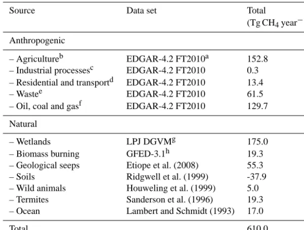
Table 4. Methane flux estimates used in the prior in the case study.
Source Data set Total
(Tg CH4year−1) Anthropogenic
– Agricultureb EDGAR-4.2 FT2010a 152.8 – Industrial processesc EDGAR-4.2 FT2010 0.3 – Residential and transportd EDGAR-4.2 FT2010 13.4 – Wastee EDGAR-4.2 FT2010 61.5 – Oil, coal and gasf EDGAR-4.2 FT2010 129.7
Natural
– Wetlands LPJ DGVMg 175.0
– Biomass burning GFED-3.1h 19.3 – Geological seeps Etiope et al. (2008) 55.3 – Soils Ridgwell et al. (1999) -37.9 – Wild animals Houweling et al. (1999) 5.0 – Termites Sanderson et al. (1996) 19.3 – Ocean Lambert and Schmidt (1993) 17.0
Total 610.0
aEmission Database for Global Atmospheric Research (http://edgar.jrc.ec.europa.eu),bIPCC categories:
4A, 4B, 4C,cIPCC category: 2,dIPCC categories: 1A3, 1A4,eIPCC categories: 6A, 6B, 6C,fIPCC categories: 1A1, 1A2, 1B1, 1B2, 7A,gLund–Potsdam–Jena Dynamic Global Vegetation Model (LPJ DGVM),hGlobal Fire Emissions Database (http://www.falw.vu/~gwerf/GFED.html).
3.1.2 Observations
We used measurements of CH4from approximately weekly samples in the National Oceanic and Atmospheric Adminis-tration Global Monitoring Division (NOAA GMD) Carbon Cycle and Greenhouse Gases (CCGG) network. These mea-surements are made using Gas Chromatographs fitted with Flame Ionization Detectors (GC-FID). In addition, we used data from a number of in situ measurement sites. These in-cluded in situ GC-FID instruments operated by the Umwelt-bundesamt (UBA), the Institute for Atmospheric Sciences and Climate (ISAC) and the Advanced Global Gases Ex-periment (AGAGE) as well as in situ Cavity Ring Down Spectrometers (CRDS) operated by EMPA and the Finnish Meteorological Institute (FMI). All measurements were re-ported as dry-air mole fractions in parts-per-billion (abbre-viated as ppb) on the NOAA2004 calibration scale, except AGAGE data, which were reported on the Tohoku Univer-sity scale but were converted to the NOAA2004 scale using a conversion factor of 1.0003 (see Table 3).
In situ measurements were assimilated as averages of the afternoon observations (12:00 to 18:00 LT) at low altitude sites and as averages of night-time observations at mountain sites (00:00 to 06:00 LT) and the corresponding FLEXPART SRRs were selected and averaged in the same way. Discrete measurements were assimilated as available and matched with the closest available 3-hourly SRR to the sampling time. The measurement error was defined as 5 ppb based on the re-peatability of the measurements and, in the case of the in situ
data, the representation error was defined as the standard de-viation of the afternoon observations.
3.1.3 Prior fluxes and initial mixing ratios
The prior flux was composed from estimates of anthro-pogenic and natural emissions from a number of different models and inventories (see Table 4 for details) and the to-tal global source amounted to 610 Tg CH4year−1. Methane fluxes were resolved monthly in the wetland, ocean, termite, wild animal, soil and biomass burning estimates, while the anthropogenic and geological flux estimates were only re-solved annually. For the anthropogenic and biomass burning sources, the 2010 estimates were used, as no estimates were available for 2011. For the remaining natural sources, cli-matological estimates were used. All fluxes were used at a spatial resolution of 1.0◦×1.0◦.
Prior flux error covariance matrix, Bflux, was calculated as described in Sect. 2.5 using a spatial correlation length of 500 km, kS=500, and a temporal correlation length of 90 days,kT=90. For the calculation of the flux errors we used a fraction of 0.5 of the maximum flux out of the cell of interest and the eight surrounding ones.
CH4mixing ratios from the atmospheric chemistry transport model, TM5, in order to calculate the initial mixing ratios. The TM5 model was run at 6.0◦×4.0◦ horizontal resolu-tion with 25 eta pressure levels using pre-optimized fields of CH4fluxes (Bergamaschi et al., 2010). Atmospheric loss of CH4 by reaction with OH radicals is calculated in TM5 using monthly fields of OH concentration (Bergamaschi et al., 2005) resulting in mean atmospheric lifetime of CH4of 10.1 years, which is close to the IPCC recommended value of 9.7 (±20 %) years (Denman et al., 2007). The initial mixing ratios were added to the change in mixing ratios from fluxes outside the domain, together forming the background mix-ing ratio matrix, Mcg(M×R). The background was optimized at a resolution of 30◦×15◦(longitude by latitude) over the global domain (i.e.R=144). The uncertainty in the scalars of the background mixing ratio was set to 0.2 % equivalent to approximately 4 ppb.
3.2 Sensitivity tests
We performed six inversions to test the sensitivity of the posterior fluxes and error reduction to the spatial correlation scale length (S1 to S3), to the optimization of the background (S4), to the filtering and averaging of the observations (S5), as well as to the background estimation method (S6). The tests are summarized in Table 5.
3.3 Results
The inversions were run on a Linux Ubuntu machine with 62 GB memory. The maximum and mean memory usage was 18 and 6.4 GB, respectively, and each inversion took approx-imately 1.8 days to complete.
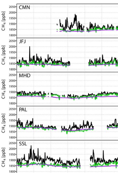
Figure 3 shows the observed CH4mixing ratios at in situ measurement sites compared with those simulated with the TM5 model and FLEXPART using the prior and posterior fluxes from test S1. At high-altitude sites, namely CMN, JFJ and SSL, the global model tends to underestimate the synop-tic variability largely due to the coarse resolution. This can be quantified by the normalized standard deviation (NSD) (i.e. the SD of the model normalized by the SD of the observa-tions), which for TM5 was 0.46, 0.81 and 0.71, compared with 0.81, 0.75 and 1.07 for FLEXPART, for the three sites respectively. On the other hand, TM5 overestimated the vari-ability at MHD, a coastal site, with a NSD of 2.53 compared with 0.97 in FLEXPART. Again, this is likely to be due to the coarse resolution in TM5, which cannot accurately re-solve the location of MHD and overestimates the influences of land fluxes at this site.
To examine the differences between the two methods of estimating the background mixing ratios, we compare the background determined in test S1 (model-based method) and test S6 (observation-based method). The results are shown in Fig. 4 at the in situ measurement sites. The two meth-ods compare reasonably well with one another with the
Figure 3. CH4mole fractions (ppb) as observed (black) and simu-lated from the prior (blue) and posterior models (red). Also shown is the background CH4mole fraction (green) and CH4calculated by the TM5 Eulerian model (light blue).
mean difference between the two backgrounds being be-tween−7 and 4 ppb for the different sites. At MHD, however, observation-based background is considerably lower than the model-based one (a difference of−11 ppb). This departure is caused by an overestimation of the prior contribution to the mixing ratio from fluxes inside the nested domain, and since this is subtracted from the observations that have been iden-tified as being representative of the background, this leads to an overall too low background estimate at this site (see Sect. 2.1.2 for details).
Table 5. Overview of the sensitivity tests.
Test ID Spatial correlation Observations Backgrounda
S1 500 km afternoon/night onlyb model-based, not optimized S2 300 km afternoon/night only model-based, not optimized S3 200 km afternoon/night only model-based, not optimized S4 500 km afternoon/night only model-based, optimized S5 500 km allc model-based, not optimized S6 500 km afternoon/night only observation-based, not optimized
aThe method of calculation and whether or not the background mixing ratios were optimized in the inversion.b Low-altitude sites averaged afternoon data, high-altitude sites averaged night data.cAveraged all data over 24 h.
Figure 4. Comparison of the background CH4mole fraction, cal-culated using the observation-based (purple) and the model-based methods (green), with the observed mixing ratio (black).
squares divided by the number of observations). Ideally,χ2
would be equal to 1 indicating that the posterior solution is within the limits of the prescribed uncertainties. In actual fact, the χ2 values are larger than 1.χ2 increased with in-creasing spatial correlation scale length with values of 2.24, 2.56 and 2.97 withkSof 200, 300 and 500 km, respectively, which is as expected since a longer correlation scale length
Table 6. Statistics of the simulated versus observed CH4 mixing ratios from test S1.
Site ID Prior Posterior
NSD R RMSE NSD R RMSE
PAL 0.99 0.69 16.2 1.04 0.82 11.9
ICE 1.01 0.26 9.4 0.90 0.24 9.2
BAL 1.14 0.66 16.6 0.96 0.72 13.7
MHD 1.18 0.57 9.2 0.97 0.63 7.8
OXK∗ – – 42.3 – – 7.34
SSL 1.21 0.52 28.2 1.07 0.71 19.3 HPB 0.61 0.49 44.3 0.67 0.73 33.7 HUN 0.54 0.69 47.5 0.96 0.88 27.1 JFJ 1.04 0.30 21.4 0.75 0.33 20.3 BSC 1.10 0.24 51.1 0.91 0.39 35.2 CMN 1.00 0.56 26.4 0.81 0.68 21.6 CIB 0.89 0.50 20.9 0.91 0.68 15.6 LMP 2.02 0.34 35.0 1.68 0.45 24.0
∗Insufficient observations for calculatingRand NSD.
corresponds to fewer degrees of freedom. Using all observa-tions, as in test S5, resulted in aχ2of 2.05, the lowest value, as this also resulted in larger SDs over the averaging inter-val (1 day) and, hence, larger uncertainties in the observation space.
Figure 5. A posteriori fluxes of CH4(left) and the flux increments (i.e. a posteriori – a priori fluxes) (right) for each of the sensitivity tests (in units of g CH4m−2day−1).
ratios have been increased (by approximately 0.2 %) to min-imize the observation–model error and, hence, smaller incre-ments were needed in the emissions. Furthermore, using all observations (test S5), compared to only afternoon ones at low-altitude sites and only night-time ones at high-altitude sites, made almost no difference to the posterior fluxes. Test S6, which used the observation-based approach for the back-ground estimation, differed the most from the other tests. No-tably, higher emissions, compared to the other inversions, were found in France, Germany, the Czech Republic and the UK and, correspondingly, the flux increments were more
positive in these regions as well. This difference is a direct result of the lower background mixing ratios estimated at a number of sites with the observation-based method and highlights the challenge of obtaining robust background esti-mates.
Figure 6 shows the error reduction for the six sensitiv-ity tests. The largest error reductions are found usingkS= 500 km, i.e. in tests S1, S4, S5 and S6, for which the error reduction is almost identical. The error reductions in tests S2 and S3 are smaller and more limited to central Europe as compared to S1. Again, this is because increasing the cor-relation scale length results in fewer degrees of freedom for the inversion and effectively spreads the atmospheric infor-mation over a larger area.
Lastly, we compare the simulated mixing ratios using the a priori and a posteriori fluxes (from test S1) with observa-tions at an independent site, i.e. one that was not included in the inversion, Puy de Dôme, France (PUY). Figure 7 shows the observed, prior, posterior and background mixing ratios at the timestamp of the observations at PUY. Both the prior and posterior mixing ratios overestimate the observed vari-ability with NSD of 2.24 and 2.04, respectively. This is most probably owing to both the topography (the station is located on a volcanic cone, which represents a very abrupt change in topography) as well as the fact that there are significant emissions in the prior around the station. A likely explana-tion is that FLEXPART overestimates the BL height at PUY and thus overestimates the influence of local emissions on this site. Despite the model transport errors at this site, using the posterior fluxes improves the RMSE (23.1) and correla-tion coefficient (0.18) compared to the prior (26.4 and 0.16, respectively).
3.4 Discussion
The results for the sensitivity tests S1 and S6, using the model and observation-based background mixing ratios, re-spectively, highlight the challenge of robustly identifying the background and the influence that this has on the optimized fluxes (see Fig. 5). There are different problems associated with each method which warrant further discussion here.
Figure 6. Error reduction for the CH4fluxes for each of the sensi-tivity tests.
Figure 7. Comparison of the prior (blue), posterior (red) and
back-ground (green) simulated CH4mixing ratios (ppb) with observa-tions (black) at the independent site, PUY. Results are shown for test S1.
one hemisphere. Furthermore, in the global model, the back-ground is constrained mainly by measurements from out-side the region of interest. The degree of circularity is min-imized even further if new observations are included in the Lagrangian inversion, which may also encompass assimilat-ing observations from the same sites but at higher temporal resolution in the Lagrangian model if observations from no additional sites are available. In any case, the model-based background should be from a pre-optimized model or op-timized in the Lagrangian inversion, as biases in the back-ground will be propagated into biases in the optimized fluxes. Second, using a filtering of the observations to derive the background will also lead to circularity, i.e. if the same ob-servations are also used to optimize the background in the inversion, and this case should be avoided. When the obser-vations are used to derive the background, biases only arise in the detection of the background signal. The background mixing ratio may fluctuate depending on the altitude and lat-itude of the air masses’ origin. In addition, if the site is in an area of strong local fluxes, a background signal may not be detectable. Analysing the modelled back-trajectories in such cases may help determine whether candidate observations for the background calculation are likely to have been influenced by fluxes in the domain or not. Furthermore, the observation-based method for determining the background is not appro-priate for species such as CO2, which have a strong diurnal cycle and thus no definable background.
Table 7. Comparison of CH4emissions (Tg CH4year−1)from this study with the range of values from an inversion ensemble for 2006 and 2007 (Bergamaschi et al., 2014). The prior and posterior emissions are shown from test S1 and include the 1σ SD prior and posterior uncertainties. NW Europe includes the UK, Ireland, BENELUX, France and Germany, and E Europe includes Hungary, Poland, the Czech Republic and Slovakia, according to the definitions in Bergamaschi et al. (2014).
Prior Posterior Bergamaschi et al. (2014)
UK+Ireland 2.66±0.84 2.41±0.33 2.32–4.57 BENELUX∗ 1.18±0.80 1.09±0.26 1.44–2.29 France 4.33±1.37 3.14±0.42 2.02–4.94 Germany 2.22±1.16 2.48±0.33 2.35–3.51 NW Europe 10.39±4.17 9.12±1.34 8.13–14.44 Hungary 0.37±0.62 0.50±0.17 0.34–0.73 Poland 2.81±1.05 2.62±0.38 1.84–2.87 Czech Republic+Slovakia 1.18±0.94 1.27±0.27 1.12–1.63 E Europe 4.36±2.61 4.39±0.82 3.59–4.90 NW+E Europe 14.75±4.17 13.51±2.16 11.71–19.34
∗BENELUX=Belgium, The Netherlands and Luxembourg.
range from the ensemble, despite differences in the time pe-riod and the atmospheric observations used. There is only one exception, i.e. BENELUX, where our estimate is 24 % lower than the lowest limit of the ensemble range. This may be due, at least in part, to real changes in emissions. How-ever, it may also be due to differing distributions of the pos-terior emissions close to the boundaries of BENELUX with France and Germany, which considering the small area of BENELUX, may become important in the calculation of the total emission. Another contributing factor may also be that in the inversions in the Bergmaschi et al. (2014) study, the station, Cabauw (52.0◦N, 4.9◦E), in the Netherlands, was in-cluded (whereas it was not inin-cluded in our inversion), which likely also has a strong influence on the posterior fluxes in BENELUX.
4 Summary and conclusions
We have presented a new Bayesian inversion framework, FLEXINVERT, for the estimation of surface to atmosphere fluxes of atmospheric species. The framework is based on source–receptor relationships, which describe the relation-ship between changes in mixing ratio at a receptor “point” and changes in fluxes, calculated by the Lagrangian Particle Dispersion Model, FLEXPART. Fluxes may be optimized at any given temporal resolution and on a nested grid of variable spatial resolution. The variable grid is determined using the information of the integrated SRRs and has finer resolution where there is a strong observational constraint and coarser resolution where there is a weak constraint. In this frame-work, the background mixing ratio, i.e. the contribution to the mixing ratio at the receptors not accounted for by transport and fluxes inside the nested domain, is calculated by coupling FLEXPART to the output of a global Eulerian model (or al-ternatively, in the case that no such model output is available,
it is calculated from the observations themselves). The back-ground mixing ratios are also included in the optimization problem.
Appendix A: Optimization of the posterior fluxes to the fine-grid resolution
To optimize the posterior fluxes fnestvg ∗ on the variable-resolution grid to the fine-variable-resolution grid by applying Bayes’ theorem (note that to simplify the notation we have used f=fnestvg ∗,fb=fnest, and f∗=fnest∗ i.e. the optimized fluxes on the fine grid),
ρ f∗f
=ρ (f|f
∗) ρ (f∗)
ρ (f) , (A1)
whereρ(f∗|f) is the posterior pdf thatf∗lies in the inter-val (f∗,f∗+df∗)whenf (the “observation”) has a given value. Assuming a Gaussian pdf and taking the natural loga-rithm we can expressρ(f|f∗)as
−2 lnρ f|f∗= f−0f∗TAflux-1 f−0f∗, (A2) (where Afluxis the posterior error covariance matrix and0is the projection operator) and we can expressρ(f∗)as
−2 lnρ f∗= f∗−fbTBflux-1 f∗−fb, (A3) (where Bfluxis the prior error covariance matrix, on the fine grid) and by substituting Eqs. (2) and (3) into Eq. (1) we derive the expression forρ(f∗|f):
−2 lnρ f∗f
= f∗−fb T
Bflux-1 f∗−fb
+ f−0f∗TAflux-1 f−0f∗. (A4) The cost function can be thus be defined as
J f∗=1
2 f ∗−f
bTBflux-1 f∗−fb +1
2 f−0f ∗T
Aflux-1 f−0f∗ (A5) and the first derivative as
J0 f∗=Bflux-1 f∗−fb
−0TAflux-1 f−0f∗. (A6)
Thus we can derive the expression forx∗at the minimum: f∗=fb
+Bfluxnaw0unitT 0Bflux0T+Aflux −1
(f−0fb) . (A7)
Appendix B: Description of the software B1 General description
The code corresponding to the inversion framework de-scribed in this paper is called FLEXINVERT and is available from the website: http://flexinvert.nilu.no under a GNU Gen-eral Public License. FLEXINVERT is coded in Fortran90
and has been tested with the gfortran compiler and the Linux Ubuntu operating system and a makefile for gfortran is in-cluded. To run FLEXINVERT, the LAPACK and NetCDF libraries for Fortran must be installed. The current version of FLEXINVERT can be run directly with output from FLEX-PART 9.2.
B2 Input data
FLEXINVERT uses two definition files, the first speci-fies the paths, filenames, and other file-related information (files.def), and the second specifies the settings for each in-version run, such as the domain, dates, and uncertainties (control.def).
– FLEXPART files
FLEXINVERT looks for FLEXPART output files for each receptor in directories with the following naming convention: /STATION/YYYYMM/ where STATION
is the name of the receptor and must be the same as that given in the station list file and in the prefix of the observation files. The FLEXPART files required are:
header, grid_time (and grid_initial when computing the background using global model out-put). It is important to note that if the full 3D SRR fields are saved in thegrid_timefiles, the reading of these files becomes considerably slower. Therefore, it is recommended to save only the surface layer of the SRR fields in the grid_time files. However, if the
grid_initialfiles are used, these need all layers. (An option for thisgrid_timeandgrid_initial
was added into FLEXPART 9.2). Also, note that FLEX-INVERT expects the stochastic errors to be written to the grid_timefiles. If these are not written then a minor modification is required inreadgrid.f90. – Station list file
This file specifies the receptors (where there are obser-vations) to include in the inversion. The default file has the following format: receptor name, latitude, longitude, altitude, observation type (either CM for continuous or FM for flask measurement) and a character string of up to 55 characters describing the receptor. However, only the receptor name and type are actually used in the in-version:
ID LAT LON ALT TYP STATIONNAME
STATION XX.XX XXX.XX XXXX XX Station Name, Country
– Observations
The files contain six columns: year, month, day, hour, minute, mixing ratio – and optionally the measurement error estimate.
– Prior fluxes
The sub-routine reademissions.f90 reads the prior fluxes (or equivalently prior emissions) from a NetCDF file containing a 3-D floating variable for the fluxes with dimensions time, latitude and longitude, and the corresponding dimension variables. The name of the floating point variable is specified in files.defby the variableemisname.
– Landcover file
FLEXINVERT uses high-resolution landcover data to specify areas of water when determining the variable resolution grid. By default, FLEXINVERT uses the IGBP data, which is included in the tar archive. – Land–sea mask file
A land–sea mask file is used in FLEXINVERT to de-termine which grid cells are on land/ocean when calcu-lating the covariance matrix. The default land–sea mask is at 0.125◦×0.125◦resolution and is converted to the needed resolution automatically.
– 3-D concentration fields
For the calculation of the initial mixing ratios from a global model, its 3-D concentration fields are needed. FLEXINVERT includes routines for reading the output of the models LMDZ4 and TM5 in NetCDF format, which can be used as templates for reading data from other models.
B3 Output data
At the end of an inversion run, FLEXINVERT writes the out-put into the following files:
– obsread.txt
ASCII file containing the observed, prior, posterior and background mixing ratios at the same timestamp as the observations. Note that if the background is not op-timized, then the observed, prior and posterior mix-ing ratios are the difference from the background and the values in the column BGND_POST are zero. The
obsread.txtfile has the following format:
ID DATE OBS PRIOR POST BGND_PRIOR BGND_POST ERROR
STATION YYYYMMDDHH F11.3 F11.3 F11.3 F9.3 F9.3 F9.3
– modout.nc
NetCDF file containing floating point variables for the prior and posterior mixing ratios (ypriandypos, re-spectively) as well as the prior and posterior background mixing ratios (bgpriandbgpos, respectively). These mixing ratios are computed using the fluxes at the finest resolution and at the timestamp of the FLEXPART tra-jectories. The variables have dimension of time and re-ceptor.
– analysis.nc
NetCDF file containing floating point variables for the prior and posterior fluxes (emis_prior and
emis_post, respectively) as well as the prior and pos-terior flux errors (error_prioranderror_post, respectively). The variables are in dimensions of longi-tude, latitude and time and have units of kg m−2s−1. – covb.nc
NetCDF file containing a floating point variable of the prior error covariance matrix (covb) and units (kg m−3s−1)2. Note that the errors are scaled by the nu-merical scaling factor defined inmod_var.f90. – cova.nc
As for covb.nc but containing the posterior error covari-ance matrix (cova).
– covr.nc
NetCDF file containing a floating point variable of the observation error covariance matrix (covr) with units of mixing ratio squared (e.g. ppb2).
– nbox_xy.nc
NetCDF file containing a floating point variable of the mapping of the fine to the variable resolution grid with dimensions of the number of longitudinal by latitudinal grid cells.
For testing purposes, the following files are also written but in most cases will not be required:
– gain.nc
NetCDF file containing the Gain matrix, BHT(HBHT+
R)−1(y−Hxb). – covbfin.nc
NetCDF file of the prior error covariance matrix on the fine grid (covbfin) with units (kg m−3s−1)2. Note that the errors are scaled by the numerical scaling factor. – covbfinaw.nc
– covagg.nc
NetCDF file of the aggregation errors in units of mixing ratio squared (e.g. ppb2).
– grid_operator.nc
NetCDF file of the projection operator,0, from the fine to the variable grid.
– grid_coarse.nc
NetCDF file of the projection operator, 0cg, from the fine to the coarse grid.
– emisflex.nc
NetCDF file of the prior emissions converted to the FLEXPART (i.e. fine) grid in units of kg m−3s−1. – knest_finobs.nc
NetCDF file of the transport operator, Hnest, for the fine grid and averaged to the observation averaging interval. – knest_obs.nc
NetCDF file of the transport operator, Hnest, for the vari-able grid and averaged to the observation averaging in-terval.
– knest_trim.nc
NetCDF file of the transport operator, Hnest, for the vari-able grid with rows matching observations.
– kout_obs.nc
NetCDF file of the initial mixing ratio contributions, Houtyout, for the coarse grid and averaged to the obser-vation averaging interval.
– immr.nc
NetCDF file of the 3-D initial mixing ratios from the global model (for option bgmethod=2 only) interpo-lated to the FLEXPART resolution (first time step only). – area_box.txt
ASCII file containing a vector of the variable grid cell areas (m2).
– prior.txt
ASCII file containing the prior state vector,xb. – posterior.txt
ASCII file containing the posterior state vector,x. – bgscalars.txt
ASCII file containing the prior and posterior scalars of the background mixing ratios and their errors with the format:
PRIOR POST PRIOR_ERROR POST_ERROR
F6.4 F6.4 F6.4 F6.4 F6.4
Appendix C: Applying inequality constraints
Acknowledgements. We thank all those who provided CH4
measurements for use in the case study, namely, E. Dlugokencky (NOAA), M. Steinbacher (EMPA), J. Arduini (ISAC), K. Uhse (UBA), J. Hatakka (FMI) and S. O’Doherty (University of Bristol). We also thank P. Bergamaschi for the use of the TM5 model output, as well as for providing the results from the inversion ensemble of CH4fluxes in Europe. In addition, we thank I. Pisso for his help improving this paper. This work was financed by the Norwegian Research Council projects SOGG-EA and GHG-Nor.
Edited by: A. Archibald
References
Belward, A. S., Estes, J. E., and Kline, K. D.: The IGBP-DIS global 1-km land-cover data set DISCover: A project overview, Pho-togram. Eng. Remote Sens., 65, 1013–1020, 1999.
Bergamaschi, P., Krol, M., Dentener, F., Vermeulen, A., Meinhardt, F., Graul, R., Ramonet, M., Peters, W., and Dlugokencky, E. J.: Inverse modelling of national and European CH4emissions us-ing the atmospheric zoom model TM5, Atmos. Chem. Phys., 5, 2431–2460, doi:10.5194/acp-5-2431-2005, 2005.
Bergamaschi, P., Krol, M., Meirink, J. F., Dentener, F., Segers, A., van Aardenne, J., Monni, S., Vermeulen, A. T., Schmidt, M., Ramonet, M., Yver, C., Meinhardt, F., Nisbet, E. G., Fisher, R. E., O’Doherty, S., and Dlugokencky, E. J.: Inverse modeling of European CH4emissions 2001-2006, J. Geophys. Res., 115, D22309, doi:10.1029/2010jd014180, 2010.
Bergamaschi, P., Corazza, M., Karstens, U., Athanassiadou, M., Thompson, R. L., Pison, I., Manning, A. J., Bousquet, P., Segers, A., Vermeulen, A. T., Janssens-Maenhout, G., Schmidt, M., Ra-monet, M., Meinhardt, F., Aalto, T., Haszpra, L., Moncrieff, J., Popa, M. E., Lowry, D., Steinbacher, M., Jordan, A., O’Doherty, S., Piacentino, S., and Dlugokencky, E.: Top-down estimates of European CH4and N2O emissions based on four different in-verse models, Atmos. Chem. Phys. Discuss., 14, 15683–15734, doi:10.5194/acpd-14-15683-2014, 2014.
Brunner, D., Henne, S., Keller, C. A., Reimann, S., Vollmer, M. K., O’Doherty, S., and Maione, M.: An extended Kalman-filter for regional scale inverse emission estimation, Atmos. Chem. Phys., 12, 3455–3478, doi:10.5194/acp-12-3455-2012, 2012.
Chevallier, F., Fisher, M., Peylin, P., Serrar, S., Bousquet, P., Bréon, F. M., Chédin, A., and Ciais, P.: Inferring CO2 sources and sinks from satellite observations: Method and application to TOVS data, J. Geophys. Res., 110, D24309, doi:10.1029/2005jd006390, 2005.
Denman, K. L., Brasseur, G. P., Chidthaisong, A., Ciais, P., Cox, P. M., Dickinson, R. E., Hauglustaine, D., Heinze, C., Holland, E., Jacob, D., Lohmann, U., Ramachandran, S., da Silva Dias, P. L., Wofsy, S. C., and Zhang, X.: Couplings Between Changes in the Climate System and Biogeochemistry, in Climate Change 2007: The Physical Science Basis. Contribution of Working Group I to the Fourth Assessment Report of the Intergovernmental Panel on Climate Change, edited by: Solomon, S. D., Qin, D., Manning, M., Chen, Z., Marquis, M., Averyt, K. B., Tignor, M., and Miller, H. L., 499–587, Cambridge University Press, Cambridge, 2007. Enting, I. G.: Inverse Problems in Atmospheric Constituent
Trans-port, Cambridge University Press, Cambridge, New York, 2002.
Etiope, G., Lassey, K. R., Klusman, R. W., and Boschi, E.: Reappraisal of the fossil methane budget and related emis-sion from geologic sources, Geophys. Res. Lett., 35, L09307, doi:10.1029/2008gl033623, 2008.
Flesch, T. K., Wilson, J. D., and Yee, E.: Backward-time Lagrangian stochastic dispersion models and their application to estimate gaseous emissions, J. App. Meteor., 34, 1320–1332, 1995. Fung, I., John, J., Lerner, J., Matthews, E., Prather, M., Steele,
L. P., and Fraser, P. J.: Three-dimensional model synthesis of the global methane cycle, J. Geophys. Res., 96, 13033–13065, doi:10.1029/91JD01247, 1991.
Gerbig, C., Lin, J. C., Wofsy, S. C., Daube, B. C., Andrews, A. E., Stephens, B. B., Bakwin, P. S., and Grainger, C. A.: To-ward constraining regional-scale fluxes of CO2with atmospheric observations over a continent: 2. Analysis of COBRA data us-ing a receptor-oriented framework, J. Geophys. Res., 108, 4757, doi:10.1029/2003jd003770, 2003.
Giostra, U., Furlani, F., Arduini, J., Cava, D., Manning, J., O’Doherty, J., Reimann, S., and Maione, M.: The determi-nation of a “regional” atmospheric background mixing ra-tio for anthropogenic greenhouse gases: A comparison of two independent methods, Atmos. Environ., 45, 7396–7405, doi:10.1016/j.atmosenv.2011.06.076, 2011.
Houweling, S., Kaminski, T., Dentener, F., Lelieveld, J., and Heimann, M.: Inverse modeling of methane sources and sinks using the adjoint of a global transport model, J. Geophys. Res., 104, 26137–26160, doi:10.1029/1999jd900428, 1999.
Kaminski, T., Heimann, M. and Giering, R.: A coarse grid three-dimensional global inverse model of the atmospheric transport: 2. Inversion of the transport of CO2in the 1980s, J. Geophys. Res., 104, 18555–18581, doi:10.1029/1999JD900146, 1999. Kaminski, T., Rayner, P. J., Heimann, M., and Enting, I. G.: On
ag-gregation errors in atmospheric transport inversions, J. Geophys. Res, 106, 4703–4715, doi:10.1029/2000JD900581, 2001. Keller, C. A., Hill, M., Vollmer, M. K., Henne, S., Brunner,
D., Reimann, S., O’Doherty, S., Arduini, J., Maione, M., Fer-enczi, Z., Haszpra, L., Manning, A. J., and Peter, T.: European emissions of halogenated greenhouse gases inferred from at-mospheric measurements, Environ. Sci. Technol., 46, 217–225, doi:10.1021/es202453j, 2012.
Koyama, Y., Maksyutov, S., Mukai, H., Thoning, K., and Tans, P.: Simulation of variability in atmospheric carbon dioxide using a global coupled Eulerian – Lagrangian transport model, Geosci. Model Dev., 4, 317–324, doi:10.5194/gmd-4-317-2011, 2011. Lambert, G. and Schmidt, S.: Reevaluation of the oceanic flux of
methane: Uncertainties and long term variations, Chemosphere, 26, 579–589, doi:10.1016/0045-6535(93)90443-9, 1993. Lauvaux, T., Gioli, B., Sarrat, C., Rayner, P. J., Ciais, P., Chevallier,
F., Noilhan, J., Miglietta, F., Brunet, Y., Ceschia, E., Dolman, H., Elbers, J. A., Gerbig, C., Hutjes, R., Jarosz, N., Legain, D., and Uliasz, M.: Bridging the gap between atmospheric concen-trations and local ecosystem measurements, Geophys. Res. Lett., 36, L19809, doi:10.1029/2009gl039574, 2009.
Manning, A. J., Ryall, D. B., and Derwent, R. G.: Estimating Euro-pean emissions of ozone-depleting and greenhouse gases using observations and a modeling back-attribution technique, J. Geo-phys. Res., 108, 4405, doi:10.1029/2002JD002312, 2003. Manning, A. J., O’Doherty, S., Jones, A. R., Simmonds, P. G., and