Impact of a time-dependent background error covariance matrix on air quality analysis

(1)

www.geosci-model-dev.net/5/1075/2012/ doi:10.5194/gmd-5-1075-2012

Geoscientific

Model Development

Impact of a time-dependent background error covariance matrix on

air quality analysis

E. Jaumouill´e1, S. Massart1, A. Piacentini1, D. Cariolle1, and V.-H. Peuch2 1_{CERFACS/CNRS-URA 1875, 31057 Toulouse, France}

2_{CNRM-Game/CNRS-URA 1357, 31057 Toulouse, France} Correspondence to: S. Massart ([email protected])

Received: 24 February 2012 – Published in Geosci. Model Dev. Discuss.: 23 April 2012 Revised: 3 August 2012 – Accepted: 6 August 2012 – Published: 6 September 2012

Abstract. In this article we study the influence of different characteristics of our assimilation system on surface ozone analyses over Europe. Emphasis is placed on the evaluation of the background error covariance matrix (BECM). Data as-similation systems require a BECM in order to obtain an op-timal representation of the physical state. A posteriori diag-nostics are an efficient way to check the consistency of the used BECM. In this study we derived a diagnostic to esti-mate the BECM. On the other hand, an increasingly used approach to obtain such a covariance matrix is to estimate it from an ensemble of perturbed assimilation experiments. We applied this method, combined with variational assimilation, while analysing the surface ozone distribution over Europe. We first show that the resulting covariance matrix is strongly time (hourly and seasonally) and space dependent. We then built several configurations of the background error covari-ance matrix with none, one or two of its components derived from the ensemble estimation. We used each of these con-figurations to produce surface ozone analyses. All the anal-yses are compared between themselves and compared to as-similated data or data from independent validation stations. The configurations are very well correlated with the valida-tion stavalida-tions, but with varying regional and seasonal charac-teristics. The largest correlation is obtained with the exper-iments using time- and space-dependent correlation of the background errors. Results show that our assimilation pro-cess is efficient in bringing the model assimilations closer to the observations than the direct simulation, but we can-not conclude which BECM configuration is the best. The im-pact of the background error covariances configuration on four-days forecasts is also studied. Although mostly positive, the impact depends on the season and lasts longer during the winter season.

1 Introduction

Data assimilation techniques are frequently used in many fields of application especially in Geosciences, such as weather forecasting and oceanography (Swinbank et al., 2003). They are used to provide an estimate of the physical state of a system consistent with the input information. This information comes from an a priori estimate of the physi-cal state (also physi-called the background) and from observations linked to the current state of the system. The assimilation output is the best estimate of the physical state given the input information. It is known as the analysis. The process that creates an analysis also involves the observational and background error covariance matrices. These matrices deter-mine the respective weights in the analysis given to each of these two pieces of information. The background matrix de-termines the spatial distribution of the correction introduced in the analysis and the balance between the control variables of the system. An optimal state can only be obtained by the assimilation process if these matrices are correctly specified (Reichle, 2008). But direct determination of the background error covariance matrix (BECM) requires information that is not directly available. It is thus important to find the appro-priate way to estimate the BECM, as it is known to strongly influence the assimilation results.

(2)

1076 E. Jaumouill´e et al.: Impact of a time-dependent background error covariance matrix on air quality analysis

Constantinescu et al. (2007) have also investigated the EnKF for the simulation of air pollution in the Northeastern United States. Alternatively, in atmospheric chemistry as in other geophysical applications, one can use a statistical interpo-lation to specify an anisotropic and heterogeneous BECM (Blond et al., 2003) or can combine an ensemble approach with a variational data assimilation approach (Massart et al., 2012; Desroziers et al., 2008; Buehner, 2005). We have used this approach for global ozone analyses, and we examine it here to provide a time-dependent BECM for a regional chem-ical application.

The goal of this paper is to investigate the impact of an ensemble-derived time-dependent BECM in regional atmo-spheric chemical data assimilation. This study contributes to the European MACC project (monitoring atmospheric com-position and climate) whose one of its goals is to provide in-formation services on European air quality. Different chem-istry and transport models (CTMs) contribute to this project to produce daily air quality forecasts for Europe and reanal-yses of European air quality. In this study we use Mocage (MOdèle de Chimie Atmosphérique à Grande Echelle), the nested-domains CTM developed at Météo-France (Peuch, 1999). Mocage is combined with an adapted version of the Centre Européen de Recherche et Formation Avancée en Cal-cul Scientifique (Cerfacs) Valentina variational data assimila-tion system (Massart et al., 2005) to produce daily analyses of surface ozone over Europe. The Mocage-Valentina varia-tional data assimilation system is combined with an ensem-ble method. We first estimate the time-dependent BECMs and in particular their variance and their correlation elements. We build several configurations of the BECM, some of them derived from the ensemble estimate. Analyses resulting from the different experiments using the different BECM models are then studied and compared. The impact of the chosen model on four day forecasts is also investigated.

The structure of this paper is as follows. In Sect. 2, the Mocage-Valentina chemical assimilation system is pre-sented, and results on an air quality case study are developed in Sects. 3 and 4. In Sect. 5, several selected experiments each using a specific background error covariance matrix are described and the impact of these experiments on the analy-sis and forecasts is studied. Conclusions and a discussion are presented in Sect. 6.

2 The background error covariance matrix in the assimilation process

In this section, the assimilation process is briefly presented. The main properties of the BECM are also given and the cho-sen methods to estimate the BECM are described.

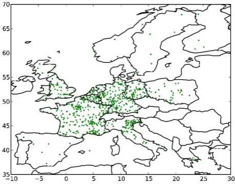
Fig. 1. Example of the location of MACC ozone ground-based stations for the 1 July 2010 .

2.1 Assimilation process

The purpose of any data assimilation method is to compute the best estimate of the unknown true state of the system studied. The estimate is usually based on the optimal combi-nation of observations and of other sources of information all gathered in a priori information. When the a priori informa-tion comes from a model, it is expressed on the model grid as the background vector xb associated with the B BECM. All the information from observations is gathered in the yo vec-tor, associated with the R observation error covariance matrix (OECM). In order to compare any state x to the observations, the possibly non-linearH observation operator is generally introduced.

The variational approach for resolving the assimilation problem consists in minimizing the variational cost function

J (x)=1

2(x−x

b₎T_B−1₍_x₋_xb₎

+1

2(y

o₋_H_x₎T_R−1₍_yo₋_H_x_{) ,} ₍₁₎

that both quantifies the difference between the current state x and the background, and the difference between the obser-vations and the equivalent in the obserobser-vations space of the model state x (Talagrand, 1997). Each difference is normal-ized by its own error specified respectively in the BECM and the OECM.

(3)

(a)

(b)

Fig. 2. Diagnosed standard deviation from a posteriori diagnostics (ppb), averaged in the period between 1 and 10 July 2010 (a) and the period between the 1 and 10 December 2010 (b).

In the case of a linear observation operator,H can be as-sociated with its matrix form H and the analysis can be ex-pressed as

xa=xb+BHTR+HBHT

−1

yo−Hxb. (2) Equation (2) shows that the analysis is equal to the back-ground plus a correction proportional to the innovation vec-tor do_b=yo−Hxb. The correction is then normalized by R+HBHT−1. The correction is reintroduced to the model space through HT and finally multiplied by B. Here, the BECM matrix, through its covariances, spreads over the model space the information coming from the observations space and extrapolated by HT _{to the model space. It includes} a spatial dispersion around the measurement location and a spread between the control model variables. This behaviour reveals it is important to have an appropriate BECM.

The OECM contains errors in the observations process, such as instrumental errors and representativeness errors. A diagonal or block diagonal OECM is used in most data as-similation applications, which assumes that the observations are loosely correlated.

(a)

(b)

Fig. 3. Diagnosed length-scales (in km) of the horizontal correla-tion of the forecast error, averaged in the period between 1 and 10 July 2010: west–east (a) and north–south (b) length-scales.

2.2 The background error covariance matrix formulation

The BECM is a key component in the data assimilation pro-cess. It contains two significant ingredients of our problem: how the observed information is spatially filtered and prop-agated, and how the control variables are correlated. The BECM is written as

B=_E(εbεbT) (3)

that merges all the information on the background error εb=xb−xt(assuming Gaussian statistics), where xtis the

true state. Equation (3) assumes that the mathematical ex-pectation_Eofεb is equal to zero. This means an unbiased

background error.

(4)

0 30 60 90 120 150 180 208 Ensembles - Ete

lpx

lp

y

Mean 12.0332 Max 208 Min 1

50 100 150 200 250 50

100 150 200 250

(a)

0 10 20 30 40 50 60 70 80 90 100 110 120 130 140 Ensembles - Hiver

lpx

lp

y

Mean 9.62618 Max 140 Min 1

50 100 150 200 250 50

100 150 200 250

(b)

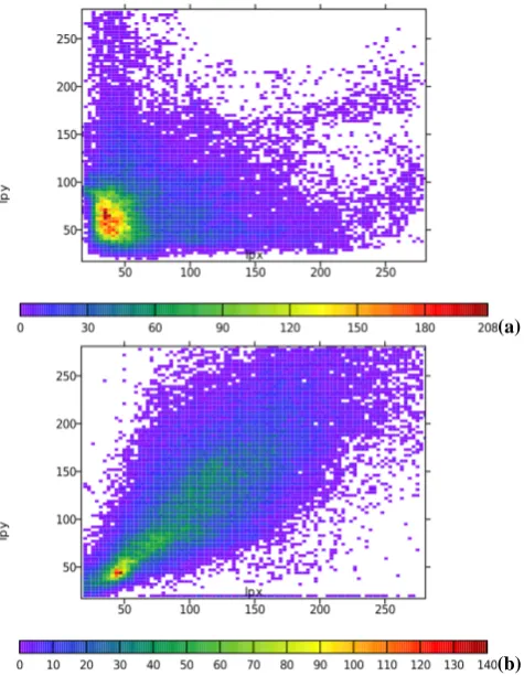
Fig. 4. Scatter diagram of length-scales (in km) of the north–south and east–west correlations of the forecast error, averaged in the pe-riod between 1 and 10 July 2010 (a) and 1 and 10 December 2010 (b); lpx represents the west–east length-scales and lpy represents the north–south length-scales.

ensemble-based method combined with variational assimi-lation as described in the following section is one of those methods.

Due to its typical size in geoscience applications (B is an

N×N matrix whereN is the dimension of the model state vector, which can reach values greater than 108), the BECM is usually written as

B=6C6T (4)

where6corresponds to the diagonal matrix of standard devi-ations of the assimilated chemical species in each grid point of the model (equal to the square root of the variances) and C corresponds to the positive definite symmetric matrix of correlations.

In order to characterize the shape of the correlation func-tions, the length-scales diagnosis is often introduced (Da-ley, 1991; Pannekoucke et al., 2008; Belo Pereira and Berre, 2006). The length-scale is considered as a relevant indica-tor of the spatial dispersion around the observation location. The larger the length-scale, the more information given by the observation is dispersed. Most of the proposed formula-tions introduced to represent the length-scales suppose that

0 5 10 15 20

Hour 20

30 40 50 60 70 80

lp

lpx (summer) lpy (summer) lpx (winter) lpy (winter)

(a)

0 5 10 15 20

Hour 20

30 40 50 60 70 80

lp

(b)

Fig. 5. Time series of estimated length-scales (in km) of the corre-lation of the forecast error, hourly-averaged in the period between 1 and 10 July 2010 and in the period between 1 and 10 Decem-ber 2010 in the grid cells of Paris (a) and Grenoble (b); lpx repre-sents the west–east length-scales and lpy reprerepre-sents the north–south length-scales.

the correlation at the origin is a Gaussian function (Constan-tinescu et al., 2007; Pannekoucke and Massart, 2008; Weaver and Ricci, 2003). Thus the correlationρbetween two points separated by a local distance ofδis

ρ(δ)=exp − δ 2

2L2 !

(5)

whereLis the length-scale.

(5)

Fig. 6. Estimated standard deviations (in ppb), averaged in the period between 1 and 10 July 2010.

0 5 10 15 20

Hour 0

2 4 6 8 10

Std

(p

pb)

Summer Winter

(a)

0 5 10 15 20

Hour 0

2 4 6 8 10

Std

(p

pb)

Summer Winter

(b)

Fig. 7. Time series of estimated standard deviations (in ppb), hourly-averaged in the period between 1 and 10 July 2010 and in the period between 1 and 10 December 2010 in the grid cells of Paris (a) and Grenoble (b).

(a)

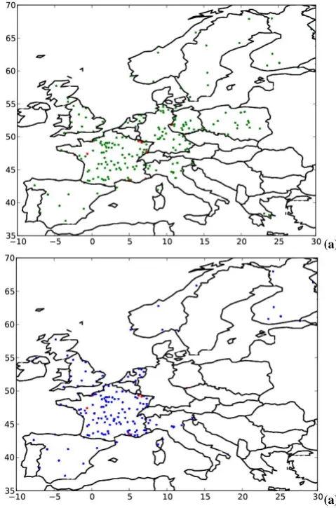
Fig. 8. Example of the location of MACC ozone rural ground-based stations, for the 1 July 2010 (a) and for the 1 December 2010 (b); the red points represent the validation stations.

2.3 BECM derived from an ensemble approach

One technique to estimate the BECM is to use an ensem-ble of variational assimilation experiments (Belo Pereira and Berre, 2006). This method consists in integrating the varia-tional data assimilation system several times on the same pe-riod with perturbed parameters (e.g. initial conditions, forc-ing, etc.). Therefore, an ensemble ofnanalysesxa_i _i₌₁_,nis obtained, wherenis the number of members of the ensemble. With a time-dependent model, forecasts are made from these analyses. These forecasts will form the background state for the next assimilation cycle. Then at each analysis time, an ensemble of backgrounds

xb_i

i=1,nis given. For each back-ground state, its difference with the mean of the ensemble of backgrounds xb₌1

n

X

i=1

xb_i gives an evaluation of the back-ground error.

(6)

backgrounds by

B'1 n

n

X

i=1

xb_i −xb _xb i −xb

T

. (6)

The standard deviations and correlations matrices can be de-duced from Eq. (6). The diagonal of the standard deviations matrix is estimated as

diag(6)= v u u t

1

n

X

i=1

xb_i −xb2_. ₍₇₎

The correlation between a grid-point k with another grid-pointlcan be written as

ρkl= 1

n6k6l

×

n

X

i=1

xb_i(k)−xb_(k) _xb

i(l)−xb(l)

(8)

where6k(resp.6l) is the background error standard devia-tions at the grid-pointk(resp.l). Assuming thatkandlare two neighbour grid-points separated by a local distance equal toδkl, the correlation obtained from Eq. (8) can be used to calculate the Gaussian length-scale using Eq. (5). Thus, the Gaussian length-scale is expressed as

Lkl=

|δkl|

√

−2 ln(ρkl(δkl))

. (9)

Belo Pereira and Berre (2006) have also proposed a rela-tively low computational cost formula for length-scale which can be used with a non Gaussian correlation:

L= s

[σ{εb(z)}]2

[σ{∂zεb(z)}]2− [∂zσ{εb(z)}]2

(10)

whereσ{εb(z)}is the standard deviation ofεb(z)and∂z=

∂/∂z, the derivative along the latitude or the longitude. Note that the formula (10) requires the computation of the forecast-error standard deviations, its gradient and the stan-dard deviation of the gradient of forecast error to calculate the length-scale.

A good estimate of the quantities in Eqs. (7) and (8) re-quires a large number of members to form the ensemble. But increasing the number of members increases the numeri-cal cost. For high resolution state-of-the-art assimilation sys-tems, the computational cost of a large number of members is too expensive. Constantinescu et al. (2007) have shown that the appropriate number of members varies, depending on the application, from about ten to some hundreds. Thus, to artifi-cially increase the number of elements on which the statistics are computed, we can compute them on several assimilation cyclescj. As an example, in the case ofmcycles, the diago-nal of the standard deviations matrix can be rewritten as

diag(6)= v u u t

1

n×m

m

X

j=1 n

X

i=1

xb_i(cj)−xb(cj)

2

. (11)

(a)

(b)

(c)

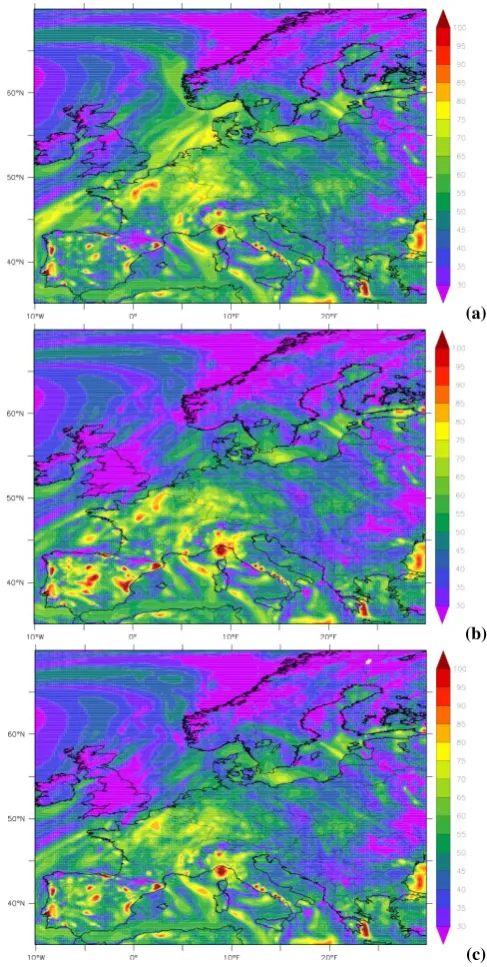
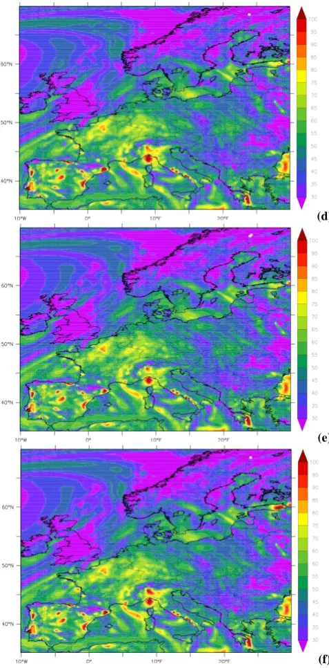
Fig. 9. Surface ozone concentration (in ppb) on the 7 July 2010 at 14:00:00 UTC for the (a) DIRECTsimulation, (b) PERCENT simu-lation, (c) OPERsimulation, see Table 1 for details on the experi-ments.

(7)

(d)

(e)

(f)

Fig. 9. Surface ozone concentration (in ppb) on the 7 July 2010 at 14:00:00 UTC for the (d) STDsimulation, (e) LXYsimulation, (f) STDLXYsimulation (continued).

2.4 BECM determination from a posteriori diagnostics Desroziers et al. (2007) introduced simple consistency di-agnostics to check covariances of observation error, back-ground error and estimation error in the observations space. These diagnostics are easily obtained since they use quanti-ties available after the analysis, such as observed values and their background and analysis counterparts in the observa-tions space. The consistency diagnostic on background errors

can be formulated as

HBHT =_E[da_b(do_b)T], (12)

with da_b the analysis-minus-background differences, do_b the innovation vector (i.e. the difference between observations and their background counterparts) and H the matrix corre-sponding to the linearized version of the observation opera-tor. Note that this diagnostic does not produce information directly on the BECM but on its projection in the observa-tions space.

Equation (12) must be satisfied if the BECM and OECM are optimum. So, generally, its left-hand side and its right-hand side are calculated separately and compared. Each side of this equation is a matrix and a common method to compare them is to compare their traces. If the traces differ, a correc-tion can be applied to the BECM to ensure identical traces and the analysis is repeated. The process can be iterated until a convergence is obtained.

Because of the expectation in the right-hand side of Eq. (12), the calculation must be done on an ensemble of data assimilation experiments in order to be significant and stable. But this turns out to be as computationally expensive as an ensemble approach.

A posteriori diagnostics are usually used to check the con-sistency of the BECM and the OECM. But since in our ap-plication the H observation operator is almost constant from one cycle to another, we replaced the computation of the ex-pectation by an average over several assimilation cycles. We also assume that the standard deviation of the background error is of the same order as the diagonal of HBHT(which is the BECM projected in the observations space). Thus, the background standard deviation in the observations space can be written as

diag(6H)'diag(HBHT) ,

' q

E[dab(d o b)T],

' v u u t

1

m

X

j=1

da_b(cj)[do_b(cj)]T (13)

wheremis the number of cycles and6His made up of the

6values from observation grid-point locations.

Similarly, the observation error covariance matrix can be di-agnosed and formulated as

diag(R)= q

E[doa(dob)T],

' v u u t

1

m

X

j=1 do

a(cj)[dob(cj)]T (14)

(8)

model grid, it would be difficult to derive the background er-ror correlation between two neighbouring model grid points from the background error correlation between two observa-tion locaobserva-tions. Thus, using the HBHTmatrix to estimate the background error correlation remains a difficult task and is out of the scope of the paper.

The above example of the use of a posteriori diagnostics to estimate the standard deviations of background and observa-tion errors is an efficient alternative to an ensemble approach. This is especially true because its computational cost is neg-ligible compared to the one of the ensemble method with the posteriori diagnostics computed over several assimilation cy-cles.

3 Numerical experiments

The numerical experiments described in this article have been done in the context of the European MACC project (MACC, 2010). Among the main MACC objectives is to provide information services covering European air qual-ity. Involved in the MACC project, Cerfacs has adapted the Mocage-Valentina data assimilation system to produce daily analysis of air quality over Europe. Several chemical species are studied within MACC but we focused on surface ozone (O3) in this study. Ozone is actively involved in atmospheric chemistry, and results from the transformation of chemical precursors by chemical and photochemical reactions. In the troposphere, ozone is one of the most relevant atmospheric pollutant indicator (Delmas et al., 2005; Finlayson-Pitts and Pitts, 2000).

3.1 The chemistry transport model

Our simulations of tropospheric and lower stratospheric chemical composition over Europe are performed with the Mocage multi-scale chemistry and transport model devel-oped at M´et´eo-France (Peuch, 1999). Mocage covers a large range of applications dealing with the study of interactions between chemistry and climate or the modelling of the tro-pospheric chemistry at a regional scale. Mocage uses me-teorological fields (e.g. wind, humidity and temperature) to compute the transport of chemical elements, the chemical and photo-dissociation rates, or the exchanges between at-mosphere and the surface. It describes the evolution of the modelled chemistry species and their horizontal and ver-tical transport in the troposphere and in the stratosphere (Josse, 2004). Among the different chemical schemes avail-able within Mocage, we chose the RACMOBUS. RAC-MOBUS is a combination of the RACM chemical scheme dedicated to the troposphere (Stockwell et al., 1997) and the REPROBUS scheme dedicated to the stratosphere (Lefevre et al., 1994). It describes the evolution of 118 modelled chemistry species. The air quality version of Mocage uses several nested domains. The largest domain is global with a

18 Jaumouill´e et al.: Impact of a time-dependent background error covariance matrix on air quality analysis

(a) Summer period

(b) Winter period

Fig. 10. Taylor diagram for several experiments studied, statistics averaged in the period between 1st and 10thJuly 2010 (top) and 1stand 10thDecember 2010 (bottom) for validation stations.

0 12 24 36 48 60 72 84

hour 0.1 0.2 0.3 0.4 0.5 0.6 0.7 0.8 correlation

Correlation Prevision 4 jours - summer

Direct Percent Oper Std Lxy StdLxy

(a) Summer period

0 12 24 36 48 60 72 84

hour 0.3 0.4 0.5 0.6 0.7 0.8 0.9 correlation

Correlation Prevision 4 jours - winter

(b) Winter period

Fig. 11. Time series of the correlation between forecasts of exper-iments studied and assimilated observations, statistics on six four-days forecasts in the period between 1st and 10thJuly 2010 (top) and 1stand 10thDecember 2010 (bottom).

(a)

18 Jaumouill´e et al.: Impact of a time-dependent background error covariance matrix on air quality analysis

(a) Summer period

(b) Winter period

Fig. 10. Taylor diagram for several experiments studied, statistics averaged in the period between 1stand 10thJuly 2010 (top) and 1stand 10thDecember 2010 (bottom) for validation stations.

0 12 24 36 48 60 72 84

hour 0.1 0.2 0.3 0.4 0.5 0.6 0.7 0.8 correlation

(a) Summer period

0 12 24 36 48 60 72 84

hour 0.3 0.4 0.5 0.6 0.7 0.8 0.9 correlation

(b) Winter period

Fig. 11. Time series of the correlation between forecasts of exper-iments studied and assimilated observations, statistics on six four-days forecasts in the period between 1st_{and 10}th_{July 2010 (top)}

and 1stand 10thDecember 2010 (bottom).

(b)

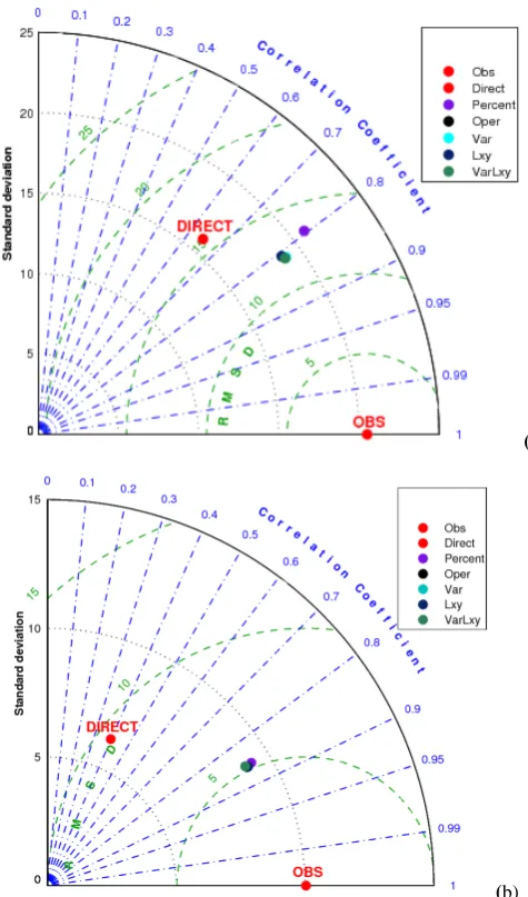
Fig. 10. Taylor diagram for several experiments studied, statistics averaged in the period between 1 and 10 July 2010 (a) and 1 and 10 December 2010 (b) for validation stations.

horizontal resolution of 2◦×2◦. It provides the boundary con-ditions for the regional domain. In our study the regional do-main covers a part of Western Europe from longitudes 16◦E to 36◦W and latitudes 32◦S to 72◦N with a horizontal res-olution of 0.2◦×0.2◦. For the two domains, the vertical res-olution has 47 levels from the ground-level to approximately 35 km.

3.2 The data assimilation system

(9)

0 12 24 36 48 60 72 84 hour

0.1 0.2 0.3 0.4 0.5 0.6 0.7 0.8

correlation

(a)

0 12 24 36 48 60 72 84 hour

0.3 0.4 0.5 0.6 0.7 0.8 0.9

correlation

(b)

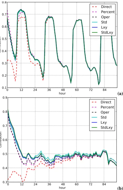
Fig. 11. Time series of the correlation between forecasts of exper-iments studied and assimilated observations, statistics on six four-days forecasts in the period between 1 and 10 July 2010 (a) and 1 and 10 December 2010 (b).

El Amraoui et al., 2010). But even if some of the previous studies performed with Mocage-Valentina were dedicated to regional aspects of the atmospheric chemical composition, they were always done with Valentina coupled with Mocage in a configuration using only its global domain. To have a regional analysis at a better resolution than the one we could extract from an analysis performed at the global scale, a specific version of Valentina has been implemented. First Valentina was coupled with the regional domain of Mocage instead of its global domain. This allowed for the perfor-mance of analysis only in the regional domain of Mocage. Used surface measurements are performed each full hour. To avoid any problem we previously encounter with the 3D-Var FGAT method when the dynamics are rapid (Massart et al., 2010), we decided to use a simple 3D-Var method that pro-duces an analysis each full hour when the data are available. Thus for each day, we have 24 successive analyses.

3.3 Ground-based stations

The ozone ground-based stations used in this study are the ones used within MACC (Airbase, 2011). They are located in Western Europe, mainly in France, Germany, Italy, Eng-land and Belgium (Fig. 1). We have chosen to study two pe-riods, one in summer and the other in winter for the year 2010. The number of reporting stations depends on the pe-riod studied. More ozone data are reported during the sum-mer period, especially in Italy, France, Sweden, Poland and Greece. The number of hourly observations varies in sum-mer (resp. in winter) between 415 (resp. 382) and 739 (resp. 687) over Europe. If several stations give measurements in the same grid cell of the model mesh during the same hour, the median value of the ozone concentrations given by these stations is assimilated. This value is allocated to the average position of all the stations used. Not all the stations provide observations every hour.

4 Estimate of the ensemble-based BECM for the surface ozone

We have used the ensemble method combined with the previously described variational assimilation to estimate an ensemble-based BECM. In the following section, the char-acteristics of the performed experiments are detailed and the results are discussed.

4.1 Characteristics of the case study

(10)

deviation is obtained for each observation location from the a posteriori diagnostic and this value is assigned to the grid cell containing the observation. An average of the standard devia-tion is also computed and assigned to all the grid cells that do not contain any observation. Then a running average of five grid cells is applied to each grid point of the whole domain. The standard deviation obtained is on average larger during the summer period than during the winter period (Fig. 2), with a mean value of 4.65 ppb in summer and 3.38 ppb in winter. The correlations used in the BECM are difficult to obtain with a posteriori diagnostics. We thus used homoge-neous and isotropic correlations by setting their length-scales to 45 km in the latitude and longitude directions. With this ozone value, variations are reflected over approximately two contiguous grid cells in each direction.

The 240 realizations obtained with the configuration de-scribed above allow the calculation of the length-scales and the standard deviation matrix using Eqs. (9) and (7), respec-tively.

4.2 The ensemble-based correlation matrix estimate From the previously described ensemble, we first diagnose the C correlation matrix of the background errors. As we for-mulate it from length-scales, we have tested the two formula-tions to calculate the scales, i.e. the Gaussian length-scales formula (Eq. 9) and the Belo Pereira and Berre for-mula (Eq. 10). As first results from the two forfor-mulations pro-vided similar values for the length-scales, we chose to use only the Gaussian formula of Eq. (9).

Atmospheric flows have generally different characteristic scales in the two horizontal directions and in the vertical. Since the correlation structures of the background error are linked to the atmospheric flow, it is essential to study the cor-relations in all directions. Nevertheless, we only focused on the horizontal direction. Diagnosing the horizontal length-scales requires the knowledge of the correlationρ(δ). It is calculated in the two horizontal directions from Eq. (8). The east–west correlation is computed using the correlation be-tween a point and its eastern neighbour. The north–south cor-relation is computed with the corcor-relation between a point and its North neighbour.

The ensemble-diagnosed length-scales show that the hori-zontal correlations are non-isotropic during summer, mainly stretched in the north–south direction (Figs. 3, 4a). The av-erage value of length-scales is 60 km in the north–south di-rection and 48 km in the east–west didi-rection. During winter, the horizontal length-scales are more isotropic (Fig. 4b). The average value of length-scales is 56 km in the north–south di-rection and 52 km in the east–west didi-rection. The values of the length-scales depend on many parameters such as wind, orography, type of grid cell (i.e. rural, urban, suburban). For example, results show that the largest length-scales are lo-cated in areas where a strong wind appears (i.e. in the Rhone valley or over Eastern Europe, figure not shown).

The isotropy is lost during summer. Larger north–south length-scales are in fact linked to the photochemical effect. At mid-latitude all the grid points along a given meridian have a zenith angle in the same range at a given time that im-plies similar photochemical effects for all these grid points, especially in summer when the photochemistry is a major component of the ozone evolution. These grid points are then correlated by the model and if we assume similar correlation in the model and its errors, then we can explain that fore-cast errors are more correlated along the meridional direction during summer. Consequently, the correlation of the forecast error is mainly isotropic, during the summer photochemical effects tending to produce anisotropy by stretching the corre-lation in the north–south direction.

The length-scale values are relatively high over Ireland, Eastern Europe, some oceanic regions and in the vicinity of domain boundaries (Fig. 3). This is related to the way the en-semble is built. First, in the vicinity of domain boundaries, when the wind is such that concentrations are influenced by boundary conditions, we lost some variability. This is for example the case for the region located West of the United Kingdom. In the upper left corner of the domain, the high values could be explained by a second phenomenon. In re-gions without observations (like oceans or Eastern Europe) the ensemble has a lower variability because of the lack of constraint by the perturbed observations. The only source of variability comes there from the perturbed emissions. And in the region of low emissions like the North West part of the North Sea, due to the low amount of emissions, perturbed emissions do not bring variability. This is less the case in some other oceanic regions where the ships produce NOx emissions that play a role in the ozone chemistry. In all the regions where the variability is low, the different simulations from all the members are thus very similar, which give a high correlation between them and results in large length-scales. To avoid too huge length-scale values, we have chosen to limit them to 200 km. Note that we also have high values for the length-scales in the Western part of the Strait of Gibraltar. There the ensemble of simulations are probably similar due to the dynamics, the strong wind advecting ozone from the Mediterranean Sea (figure not shown).

(11)

by the ozone photochemistry. In the Rhone valley during winter, the high north–south length-scales compared to the observed average values (Fig. 5b) may be due to the rapid ozone transport associated to the Mistral (a high North–South wind very common in the Rhone valley).

4.3 The ensemble-based standard deviation matrix estimate

We have also used the ensemble of backgrounds created from the different members of the ensemble approach to calcu-late the standard deviation part of the BECM with Eq. (11). The ensemble-diagnosed standard deviations are inhomoge-neous over Europe (Fig. 6). As already explained in the pre-vious section, where there is no constraint by the perturbed observations and near the boundaries of the domain (like Eastern Europe) or over a region with low emissions (like North Sea), we have low variability in the ensemble that re-sults in low standard deviation. Note that over the Mediter-ranean Sea, in spite of the absence of observations, we pro-duce some variability thanks to the perturbation of the emis-sions (from ships). Other geophysical features appear such as over the Alps, the Rhone valley and the largest cities in Spain and Italy during summer. The same structures ap-pear over Europe during winter with a smaller average of the standard deviations, 4.85 ppb (against 5.05 ppb for summer). Larger standard deviations during the summer season could be due to high ozone concentration and variability. The anti-cyclonic condition over Europe during this period (figure not shown) leads to this chemical situation. A diurnal variation is observed during summer with an increase during the day. During winter, the variations of the standard deviations are smooth and the diurnal cycle is not visible (Fig. 7).

We can remark that the structure of the standard deviations obtained with the ensemble approach over Europe presents much higher spatial variations than the ones used to build the ensemble members (i.e. obtained with the a posteriori diag-nostics shown in Fig. 2). The values estimated with our en-semble approach are larger than the diagnosed standard devi-ations values. We have likely chosen too large a standard de-viation to perturb the emissions used to create the ensemble members. Thus, the standard deviations from the ensemble approach are too large.

5 Impact of the BECM on surface ozone

The ensemble-based diagnosed BECM indicates that this error is space- and time-dependent with sometimes large diurnal variations. So a time-dependent BECM should be adopted in our system to ensure a good surface ozone anal-ysis. To measure the impact of such a time-dependent ma-trix and the impact of each of its components on the analysis of surface ozone over Europe, we performed the following study. Five experiments were performed based on BECMs

modelled using for its components a simple formulation, a posteriori diagnostics, or ensemble-based estimations. Statis-tics on the five analyses and five forecasts from the five ex-periments are computed against a selection of validation sta-tions. They are also used to estimate the most relevant con-figuration of the BECM for our case study.

5.1 The BECM experiments

Five experiments that differ only by the choice of the BECM configuration have been conducted. These experiments have been chosen to identify the influence of each BECM parame-ters (i.e. the length-scales and the standard deviations). These experiments are the following:

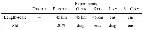
– PERCENT: the standard deviations of the BECM used for this experiment are taken as a percentage of the background, i.e. 20 %. This makes the BECM time-dependent as the background changes. The horizontal length-scales are homogeneous in latitude and longi-tude. This value is constant and set to 45 km for each grid point and has no diurnal variation.

– OPER: the standard deviations used to build the BECM are derived from the a posteriori diagnostics computed in the month before the period studied (Desroziers di-agnostics detailed in Sect. 2). The BECM is time-independent. As in the PERCENT experiment, the hor-izontal length-scales are taken as homogeneous and equal to 45 km. This experiment is the operational (OPER) configuration routinely used within the Euro-pean MACC project.

– STD: the standard deviations used in the BECM for this experiment are those which were estimated from the en-semble method described in the previous section. As in the OPERand the PERCENT experiments, the horizon-tal length-scales are equal to 45 km in latitude and in longitude.

– LXY: in this experiment, the horizontal length-scales used to model the BECM are set to the values obtained from the ensemble-based estimation. The correlation matrix is time- and space-dependent. The standard de-viations used in the BECM are the same as the OPER experiment.

– STDLXY: in this experiment, the BECM is modelled us-ing both the length-scales and the standard deviations which were estimated from the ensemble of realizations described in the previous section. This experiment cor-responds to a fully time-dependent BECM.

To evaluate the impact of these five experiments, we also used the Mocage run without assimilation. This simulation is our reference and is called the DIRECTexperiment.

(12)

Table 1. Summary of the experiments used to identify the influence of the BECM parameters. “diag.” means that the parameter was calculated from a posteriori diagnostics; “ens.” means that the parameter was calculated from an ensemble of realizations.

Experiments

DIRECT PERCENT OPER STD LXY STDLXY

Length-scale – 45 km 45 km 45 km ens. ens.

Std – 20 % diag. ens. diag. ens.

Table 2. Coordinates of the validation stations; 1–5 both for summer and winter periods, 6–10 only for summer period, 11 only for winter period; FR for France and GE for Germany.

1 2 3 4 5

FR FR FR FR GE

(47.42,-0.61) (49.16,6.65) (49.33,6.27) (49.35,0.11) (50.43,12.61)

6 7 8 9 10

FR FR FR FR GE

(43.45,4.93) (43.65,7.20) (47.27,-2.34) (47.74,7.30) (51.8,10.62)

11 FR (43.51,4.98)

5.2 Assimilated stations

From the MACC ozone ground-based stations presented in Sect. 3, a selection of station was done. A classification by type of stations (i.e. urban, suburban and rural) has been de-veloped at Centre National de Recherches Météorologiques (CNRM) by Joly and Peuch (2012). This classification in ten classes is based on the measurement data itself, using all the data available in the European AirBase data set and the French data set named BDQA (Base De données de Qualité de l’Air, i.e. Air Quality Data Base). Each class allows to group past time series of measured pollutants that are homo-geneous from the point of view of their statistical properties. Thanks to this classification we retain exclusively rural sta-tions in the assimilation process. Rural stasta-tions give a rele-vant representation of large-scale conditions because they are less influenced by local phenomena (e.g. emissions).

The ozone rural ground-based stations are mainly located in Western Europe. An example of rural station locations is shown in Fig. 8. The number of hourly rural observations varies in summer (resp. in winter) between 206 (resp. 152) and 255 (resp. 247) over Europe.

5.3 Validation stations

From the rural selection of assimilated stations, some sta-tions were excluded from the assimilation process to serve as independent validation stations. We selected a validation station if its grid mesh contains more than three stations. The number of these validation stations depends on the season studied: 10 during summer and 6 during winter (red points in

Fig. 8). The coordinates of these stations are given in Table 2. Each day, the observations from the validation stations vary from 138 to 167 during summer, and from 72 to 95 during winter.

5.4 Results for the assimilated stations

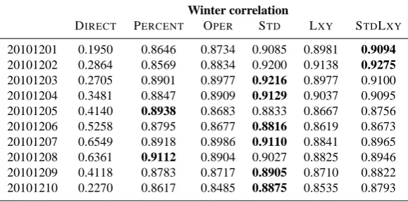
The daily correlation between the analysis of each experi-ment and the assimilated observations are given in Tables 3 and 4 for the two periods studied. The correlation of the five assimilation experiments is relatively high (around 0.9) and is always larger than the correlation obtained with the direct Mocage run (i.e. the DIRECTexperiment). The values of the correlation from the DIRECTexperiment show large seasonal variations. During the winter period, the daily correlation is sometimes very low, as an example around 0.2 for the pe-riod 1 to 10 December 2010. This is likely due to the diffi-culty of the Mocage model to account for low ozone concen-trations. However, during the summer period, high peaks of ozone concentration are well modelled and the correlation is higher (around 0.7).

(13)

Table 3. Daily correlation between analysis of the experiments studied and assimilated observations, statistics during the period between 1 and 10 July 2010; the largest daily correlation is in bold.

Summer correlation

20100701 0.7121 0.9120 0.8915 0.8989 0.8951 0.9056 20100702 0.7242 0.9003 0.8929 0.8939 0.8936 0.8966 20100703 0.6183 0.8923 0.8898 0.8940 0.8924 0.8945 20100704 0.5939 0.8924 0.8779 0.8864 0.8900 0.9051 20100705 0.6376 0.9382 0.9205 0.9236 0.9254 0.9248 20100706 0.5791 0.9306 0.9075 0.9115 0.9111 0.9168 20100707 0.6905 0.9493 0.9311 0.9366 0.9372 0.9387 20100708 0.6641 0.8924 0.8860 0.8879 0.8902 0.8945 20100709 0.6972 0.9044 0.9056 0.9112 0.9056 0.9099 20100710 0.7184 0.9269 0.9016 0.9059 0.9030 0.9089

Table 4. Same as Table 3 with statistics on the period between 1 and 10 December 2010.

Winter correlation

20101201 0.1950 0.8646 0.8734 0.9085 0.8981 0.9094 20101202 0.2864 0.8569 0.8834 0.9200 0.9138 0.9275 20101203 0.2705 0.8901 0.8977 0.9216 0.8977 0.9100 20101204 0.3481 0.8847 0.8909 0.9129 0.9037 0.9095 20101205 0.4140 0.8938 0.8683 0.8833 0.8667 0.8756 20101206 0.5258 0.8795 0.8677 0.8816 0.8619 0.8673 20101207 0.6549 0.8918 0.8986 0.9110 0.8841 0.8965 20101208 0.6361 0.9112 0.8904 0.9027 0.8825 0.8946 20101209 0.4118 0.8783 0.8717 0.8905 0.8710 0.8822 20101210 0.2270 0.8617 0.8485 0.8875 0.8535 0.8793

The two LXYand STDLXYexperiments also produce high correlation values compared to assimilated data. As the length-scales of the BECM are larger for these experiments than the length-scales of the others, we deduced that increas-ing the correlation length-scales of the background error al-lows to better represent the assimilated data.

Note that we only discuss in this paper the correlation be-tween different sets of observations. We do not discuss other statistical diagnostics. But we nevertheless systematically checked the root-mean-square statistic (RMS), as we found a similar behaviour for the correlation and the RMS, the results on the RMS will not be discussed in this paper.

Even if statistical results compared to assimilated data are close for each experiment, we observed significant differ-ences on individual analysis. For example, surface ozone fields over Europe on the 7 July 2010 at 14:00:00 UTC are represented in Fig. 9 for the six experiments studied. Common features are observed: the highest ozone concen-trations arise where the assimilated stations are located and high peaks of ozone are visible over the most polluted places (e.g. over big cities). The DIRECTexperiment mostly under-estimates the ozone concentrations on these polluted places. Comparing the DIRECTexperiment with the various analyses

shows that the Mocage model tends to produce more ozone at the surface than the analyses, even over places where the analyses are not constrained by the observations (e.g. in Eng-land and Eastern Europe, figures not shown). In the exper-iments with a horizontal length-scales equal to 45 km (i.e. the PERCENT, OPER and STD experiments), large differ-ences are observed in the ozone fields in the vicinity of large cities, such as over Paris, Milano, Madrid or Valencia. The ozone fields agree better when the standard deviations ma-trix is diagnosed with a posteriori diagnostics (i.e. the OPER experiment) or is estimated from the ensemble of realiza-tions (i.e. the STD experiment). The distribution of ozone over the Alps and urban cities is also quite similar when the ensemble-based correlation matrix is used (i.e. the LXYand STDLXYexperiments). The surface ozone in the polluted ar-eas varies between the five experiments and depends on both correlation and standard deviation matrices.

5.5 Results for the validation stations

(14)

independent validation stations. This type of diagnostic sum-marises well the statistics of the analysed fields from the six experiments in comparison with the reference field obtained from the validation stations. The position of each point quan-tifies how closely the analysis pattern matches observations. The correlation of an analysis and the observation patterns is indicated on the radius of the diagram. The standard devia-tion of an analysis is propordevia-tional to the radial distance from the origin. The centred root-mean-square difference between an analysis and the observation pattern is proportional to the distance to the point on the x-axis identified as “OBS”.

All the experiments issued from the assimilation process have a better RMS and a standard deviation closer with re-spect to the observations than the DIRECTexperiment. The 10-days correlations between analyses and the validation sta-tions are lower than the correlasta-tions between analyses and the assimilated stations. This means that the analysis is not able to constrain the values in the grid-cells which are too far from the assimilated stations. The five experiments issued from as-similation have a large correlation, ranging from 0.8 to 0.85 (Fig. 10) during the two periods studied. The statistics of the five experiments are very similar during the winter period (Fig. 10b), but show more spread in summer (Fig. 10a). The largest correlation is obtained when the length-scales vary in the BECM. During summer the largest correlation is given by the VARLXYexperiment and during winter by the LXY ex-periment. A systematic bias (i.e. the difference between the mean of the analysis and the mean of the observations) ap-pears in the Mocage model, larger during the winter period than during the summer period (−3.37 ppb in winter against

−1.62 in summer). The bias is reduced thanks to the five experiments issued from the assimilation process during the winter period but the bias is larger with these experiments during the summer period (figures not shown).

Those diagnostics clearly show that our assimilation pro-cess is efficient to bring the model closer to the observations than the direct simulation, but we cannot conclude at this stage which BECM configuration is the best.

5.6 The impact of the BECM experiments on forecasts To assess the differences between the models used for the BECM, we also studied the impact of our experiments on the ozone forecasts. To this end, six forecasts of four days (i.e. using Mocage without an assimilation technique) are created for each assimilated experiment. The first forecast begins on the first day of the period studied; the second forecast begins the day 2 of the period studied; etc. For each forecast, the initial conditions come from the analysis. Thus, six forecasts of 96 h are obtained for each assimilated experiment.

In parallel, six four-day forecasts of the DIRECT exper-iment are obtained from the Mocage simulation without assimilation. The first forecast is made up of the days 1 to 4 of the Mocage simulation; the second forecast is made up of the days 2 to 5 of the Mocage simulation; etc.

The hourly correlations between the six 96 h forecasts and the assimilated observations are calculated. Thus, the value of the correlation at 1 h represents the mean of the correla-tions of the first hour of the six forecasts.

Improvements in ozone forecasts subsequent to the assim-ilation procedure were found as in the studies of Elbern and Schmidt (2001) and Blond and Vautard (2004). In our study, results indicate that the impact of the assimilation process persists longer during the winter period than the summer period: one day in summer and about three days in winter (Fig. 11). After that, forecasts from the five experiments from the assimilations are very similar to the DIRECTsimulation. These results are consistent with the study of Blond and Vau-tard (2004) which shows that ozone analysis initialization improves the simulation for 24–48 h later and beyond that time the analysis becomes identical to the simulation with-out assimilation. During the first 12 h, the influence of our assimilation is rapidly reduced for the winter period. In sum-mer, large daily variations of the correlation coefficient are observed, but the analyses from the five experiments are all better than the direct simulation for the first day. During sum-mer nights, Mocage does not model well the ozone evolution and gives low correlations (less than 0.2). During the winter period studied, the Mocage simulation starts with a correla-tion equal to 0.3 that grows the days after. As the correlacorrela-tion with the observations of the 1 December 2010 is very low (see Table 4), the mean of the six analyses is significantly re-duced as the beginning of the 96 h forecast correlation, and the correlation profile of the Mocage simulation is not close to the profile of the other experiments.

6 Conclusions and future work

In this paper we have studied the impact on surface ozone analysis of a time-dependent background error covariances matrix. In our approach the BECM is constructed from a combination of a correlation and a standard deviations ma-trices, the correlations being characterized by length-scales. To evaluate our BECM model, we diagnose the standard-deviations and the length-scales using an ensemble approach and a posteriori diagnostics.

The diagnostics from the ensemble approach have shown that over Europe the length-scales and the standard devia-tions of the forecast error vary significantly spatially and temporally (both hourly and seasonally). These variations are larger during the summer period than during the winter pe-riod because the ozone concentration and its variations are photochemically driven. The values of the standard devia-tions estimated with the ensemble approach are larger than the diagnosed standard deviations with a posteriori diagnos-tics. The standard deviation used to perturb the emissions to create the ensemble members is likely too large.

(15)

and standard deviations matrices come from the ensemble-based diagnostics or from a posteriori diagnostics. The re-sults from these experiments are compared to a simulation without assimilation, and to a simpler experiment in which the standard deviation is equal to a percentage of the back-ground field and the length-scales are fixed. All the analyses from these experiments are very correlated to the observa-tions, the data assimilated or the independent validation tions. Comparisons of the analyses with the validation sta-tions show that the use of a BECM with time-dependent length-scales gives the largest correlation. All the analyses have a better correlation with the observations than the di-rect Mocage simulation, but the differences between them are small and we cannot conclude which BECM formula-tion is the most appropriate to the ozone simulaformula-tion over Eu-rope. The correlation depends on the period studied and may change from one day to another. Finally, the impact of the BECM formulation on four-days forecasts has been studied. Our assimilation process has a different time influence on the ozone forecasts depending on the period: one day during the summer season, three days during the winter season. For longer forecasts, the simulations from the analyses appear to have no added value compared to the direct Mocage simula-tion.

However our results have been obtained for rather limited periods. It remains to be seen how the present statistics would evolve for multi-year analyses. The impact of the BECM formulation has been also difficult to evaluate because the Mocage model shows a systematic bias in situations with low ozone concentration. So the impact of the analysis process is mostly to remove this bias, but this appears to be insuf-ficient to improve the forecast beyond one day. It would be therefore interesting to evaluate the influence of the BECM formulation following the same methodology, but with other chemistry transport models with different error characteris-tics.

Acknowledgements. The authors would like to thank William Lahoz for the constructive comments on this paper.

Edited by: K. Gierens

The publication of this article is financed by CNRS-INSU.

References

Airbase: The European air quality database (version 5), http://www.eea.europa.eu/data-and-maps/data/ airbase-the-european-air-quality-database-3, last access: 22 February 2012, 2011.

Barret, B., Ricaud, P., Mari, C., Atti´e, J.-L., Bousserez, N., Josse, B., Le Flochmo¨en, E., Livesey, N. J., Massart, S., Peuch, V.-H., Piacentini, A., Sauvage, B., Thouret, V., and Cammas, J.-P.: Transport pathways of CO in the African upper troposphere during the monsoon season: a study based upon the assimilation of spaceborne observations, Atmos. Chem. Phys., 8, 3231–3246, doi:10.5194/acp-8-3231-2008, 2008.

Belo Pereira, M. and Berre, L.: The use of an Ensemble approach to study the Background Error Covariances in a Global NWP model, Mon. Wea. Rev., 134, 2466–2489, 2006.

Blond, N. and Vautard, R.: Three-dimensional ozone analyses and their use for short-term ozone forecasts, J. Geophys. Res, 109, D17303, doi:10.1029/2004JD004515, 2004.

Blond, N., Bel, L., and Vautard, R.: Three-dimensional ozone data analysis with an air quality model over the Paris area, J. Geophys. Res, 108, 1993–1996, 2003.

Buehner, M.: Ensemble-derived stationary and flow-dependent background-error covariances: Evaluation in a quasi-operational NWP setting, Q. J. Roy. Meteorol. Soc., 131, 1013–1043, 2005. Buis, S., Piacentini, A., and D´eclat, D.: PALM: a computational

framework for assembling high-performance computing appli-cations, Concurrency and computation: practice and experience, 18, 231–245, 2006.

Claeyman, M., Atti´e, J.-L., El Amraoui, L., Cariolle, D., Peuch, V.-H., Teyss`edre, V.-H., Josse, B., Ricaud, P., Massart, S., Piacentini, A., Cammas, J.-P., Livesey, N. J., Pumphrey, H. C., and Edwards, D. P.: A linear CO chemistry parameterization in a chemistry-transport model: evaluation and application to data assimilation, Atmos. Chem. Phys., 10, 6097–6115, doi:10.5194/acp-10-6097-2010, 2010.

Coman, A., Foret, G., Beekmann, M., Eremenko, M., Dufour, G., Gaubert, B., Ung, A., Schmechtig, C., Flaud, J.-M., and Berga-metti, G.: Assimilation of IASI partial tropospheric columns with an Ensemble Kalman Filter over Europe, Atmos. Chem. Phys., 12, 2513–2532, doi:10.5194/acp-12-2513-2012, 2012.

Constantinescu, E., Sandu, A., Chai, T., and Carmichael, G.: Ensemble-based chemical data assimilation. I: General approach, Q. J. Roy. Meteorol. Soc, 133, 1229–1243, 2007.

Daley, R.: Atmospheric data analysis, Cambridge atmospheric and space sciences series, Cambridge University Press, 457, 1991. Delmas, R., M´egie, G., and Peuch, V.: Physique et chimie de

l’atmosph`ere, Belin, 608, 2005.

Desroziers, G., Berre, L., Chapnik, B., and Poli, P.: Diagnosis of ob-servation, background and analysis-error statistics in observation space, Q. J. Roy. Meteorol. Soc., 131, 3385–3396, 2007. Desroziers, G., Berre, L., Pannekoucke, O., Stefanescu, S.,

Brousseau, P., Auger, L., Chapnik, B., and Raynaud, L.: Flow-dependent error covariances from variational assimilation en-sembles on global and regional domains, Hirlam Technical Re-portY, 68, 2–22, 2008.

(16)

and MOPITT CO assimilated fields, Atmos. Chem. Phys., 10, 2175–2194, doi:10.5194/acp-10-2175-2010, 2010.

Elbern, H. and Schmidt, H.: Ozone episode analysis by four-dimensional variational chemistry data assimilation, J. Geophys. Res., 106, 3569–3590, 2001.

Elbern, H., Schwinger, J., and Botchorishvili, R.: Chemical state estimation for the middle atmosphere by four-dimensional varia-tional data assimilation: System configuration, J. Geophys. Res, 115, D06302, doi:10.1029/2009JD011953 , 2010.

Finlayson-Pitts, B. and Pitts, J.: Chemistry of the upper and lower atmosphere: Theory, experiments, and applications, Academic Pr, 2000.

Joly, M. and Peuch, V.-H.: Objective classification of air quality monitoring sites over Europe, Atmos. Environ., 47, 111–123, 2012.

Josse, B.: Représentation des processus de transport et de lessivage pour la modélisation de la composition chimique de l’atmosphère à l’échelle planétaire, Ph.D. thesis, Université Paul Sabatier, Toulouse (UPS), 2004.

Lefevre, F., Brasseur, G., Folkins, I., Smith, A., and Simon, P.: Chemistry of the 1991–1992 stratospheric winter: Three-dimensional model simulations, J. Geophys. Res., 99, 8183– 8195, 1994.

MACC: Monitoring Atmospheric Composition and Climate, http: //www.gmes-atmosphere.eu/, (last access: 2 August 2012), 2010. Massart, S., Cariolle, D., and Peuch, V.-H.: Vers une meilleure représentation de la distribution et de la variabilité de l’ozone at-mosphérique par l’assimilation des données satellitaires, CRAS, 337, 1305–1310, 2005.

Massart, S., Clerbaux, C., Cariolle, D., Piacentini, A., Turquety, S., and Hadji-Lazaro, J.: First steps towards the assimilation of IASI ozone data into the MOCAGE-PALM system, Atmos. Chem. Phys., 9, 5073–5091, doi:10.5194/acp-9-5073-2009, 2009.

Massart, S., Pajot, B., Piacentini, A., and Pannekoucke, O.: On the merits of using a 3D-FGAT assimilation scheme with an outer loop for atmospheric situations governed by transport, Mon. Wea. Rev., 4509–4522, doi:10.1175/2010MWR3237.12010. Massart, S., Piacentini, A., and Pannekoucke, O.: Importance of

using ensemble estimated background error covariances for the quality of atmospheric ozone analyses, Q. J. Roy. Meteor. Soc., 138, 889–905, doi:10.1002/qj.971, 2012.

Pannekoucke, O. and Massart, S.: Estimation of the local diffusion tensor and normalization for heterogeneous correlation mod-elling using a diffusion equation, Q. J. Roy. Meteor. Soc., 134, 1425–1438, 2008.

Pannekoucke, O., Berre, L., and Desroziers, G.: Background-error correlation length-scale estimates and their sampling statistics, Q. J. Roy. Meteorol. Soc., 134, 497–508, 2008.

Peuch, V.-H., Amodei, M., Barthet, T., Cathala, M.-L., Josse, B., Michou, M., and Simon, P.: MOCAGE : Modèle de Chimie-Transport à Grande Echelle, in: Acte de l’Atelier de Modélisation de l’Atmosphère, 33–36, 1999.

Reichle, R.: Data assimilation methods in the Earth sciences, Adv. Water Resour., 31, 1411–1418, 2008.

Stockwell, W., Kirchner, F., Kuhn, M., and Seefeld, S.: A new mechanism for regional atmospheric chemistry modeling, J. Geophys. Res., 102, 25847–25879, 10.1029/97JD00849, 1997. Swinbank, R., Shutiev, V., and Lahoz, W.: Data assimilation for the

earth system, 26, Springer Netherlands, 2003.

Talagrand, O.: Assimilation of observations, an introduction, J. Me-teorol. Soc. Jpn, 75, 81–99, 1997.