www.geosci-model-dev.net/9/3779/2016/ doi:10.5194/gmd-9-3779-2016
© Author(s) 2016. CC Attribution 3.0 License.
Development and evaluation of a high-resolution reanalysis of the
East Australian Current region using the Regional Ocean Modelling
System (ROMS 3.4) and Incremental Strong-Constraint
4-Dimensional Variational (IS4D-Var) data assimilation
Colette Kerry1, Brian Powell2, Moninya Roughan1, and Peter Oke3
1University of New South Wales, Sydney, NSW, 2052, Australia 2University of Hawai’i at Manoa, Honolulu, Hawaii, USA 3CSIRO Marine and Atmospheric Research, Hobart, Australia
Correspondence to:Colette Kerry ([email protected])
Received: 22 February 2016 – Published in Geosci. Model Dev. Discuss.: 3 March 2016 Revised: 15 September 2016 – Accepted: 25 September 2016 – Published: 26 October 2016
Abstract. As with other Western Boundary Currents glob-ally, the East Australian Current (EAC) is highly variable making it a challenge to model and predict. For the EAC re-gion, we combine a high-resolution state-of-the-art numeri-cal ocean model with a variety of traditional and newly avail-able observations using an advanced variational data assimi-lation scheme. The numerical model is configured using the Regional Ocean Modelling System (ROMS 3.4) and takes boundary forcing from the BlueLink ReANalysis (BRAN3). For the data assimilation, we use an Incremental Strong-Constraint 4-Dimensional Variational (IS4D-Var) scheme, which uses the model dynamics to perturb the initial con-ditions, atmospheric forcing, and boundary concon-ditions, such that the modelled ocean state better fits and is in balance with the observations. This paper describes the data assimilative model configuration that achieves a significant reduction of the difference between the modelled solution and the obser-vations to give a dynamically consistent “best estimate” of the ocean state over a 2-year period. The reanalysis is shown to represent both assimilated and non-assimilated observa-tions well. It achieves mean spatially averaged root mean squared (rms) residuals with the observations of 7.6 cm for sea surface height (SSH) and 0.4◦C for sea surface tempera-ture (SST) over the assimilation period. The time-mean rms residual for subsurface temperature measured by Argo floats is a maximum of 0.9◦C between water depths of 100 and 300 m and smaller throughout the rest of the water column. Velocities at several offshore and continental shelf moorings
1 Introduction
The East Australian Current (EAC) is the Western Boundary Current (WBC) of the South Pacific subtropical gyre, flow-ing poleward along the east coast of Australia. The EAC has the weakest mean flow of the WBCs associated with the sub-tropical gyres (Mata et al., 2000) but its flow is characterised by high eddy variability (Mata et al., 2006) comparable with stronger WBCs such as the Gulf Stream, the Kuroshio and the Agulhas Current (e.g. Gordon et al., 1983; Feron, 1995). The EAC forms in the South Coral Sea (15–24◦S) and in-tensifies as it flows along the coast of south-east Queensland and northern New South Wales (NSW) (22–35◦S) – refer to Fig. 1 for geographical location. The current strengthens as the continental shelf narrows to 15 km at its narrowest point (31◦S) and typically separates from the coast between 31 and 33◦S (Cetina Heredia et al., 2014). Turning eastward to form
the Tasman Front, the current sheds large warm- and cold-core eddies in the Tasman Sea every 90–110 days (Oke and Middleton, 2000; Cetina Heredia et al., 2014). The high eddy variability makes the EAC a challenging system to observe and predict.
In general, the kinetic energy of the ocean is dominated by submesoscale and mesoscale eddies that fluctuate on timescales of days to months and on spatial scales of tens to hundreds of kilometres and exceeds the mean flow by 1 order of magnitude or more (Stammer, 1997; Ferrari and Wunsch, 2009). Eddies are typically generated by barotropic or baroclinic instabilities, which are difficult to forecast; therefore, effective state-estimation and prediction of the mesoscale circulation requires data assimilation techniques that combine ocean observations with a dynamical model. Much of the effort towards data assimilative modelling of the EAC region has been part of the development of Aus-tralia’s Bluelink Ocean Data Assimilation System (BODAS) (Oke et al., 2005, 2008, 2013) which uses an Ensemble Op-timal Interpolation (EnOI)-based scheme. The BODAS has been a useful and relatively efficient method to provide ocean state estimates of the Australian region. EnOI uses long-run statistics to generate the covariance of model points and as-similates observations at a single time to generate adjusted initial conditions for each assimilation window. O’Kane et al. (2011) present an ensemble prediction study of the EAC re-gion and identify rere-gions of instability associated with the Tasman Front and EAC extension.
In this work we use Incremental Strong-constraint 4-Dimensional Variational data assimilation (IS4D-Var), which generates increments to adjust the model initial conditions, boundary and surface forcings such that the difference be-tween the model solution of the time-evolving flow and all available observations is minimised over an assimilation in-terval. The 4D-Var scheme uses the linearised model equa-tions and their adjoint to compute the increment adjustments, such that the model is adjusted in a dynamically consis-tent way to minimise the difference between the
observa-tions and the modelled time-evolving ocean state. Using the linearised equations allows dynamical connections between state variables to propagate information from observed vari-ables to unobserved, dynamically linked varivari-ables. Because the linearised version of the governing equations is used, rather than the full nonlinear version, the assimilation inter-val length is limited such that the linear assumption remains reasonably valid and the nonlinearities do not grow too large. The state estimate is a solution of the model equations, and the minimisation process can be used to understand the sensi-tivity of the modelled ocean circulation to initial conditions, boundary and surface forcing, and model parameters (e.g. Moore et al., 2009; Powell et al., 2012). Zavala-Garay et al. (2012) used 4D-Var with ROMS to assimilate sea surface height (SSH), sea surface temperature (SST), and Expend-able Bathythermograph (XBT) observations into a coarse-resolution (18–30 km) model of the EAC region. They use an empirical relationship between surface and subsurface prop-erties to help propagate the dominant surface observations to the subsurface and improve their subsurface estimates.
Combining a state-of-the-art numerical ocean model with a variety of traditional and newly available observations, we generate a high-resolution ocean state estimate of the EAC region over a 2-year period (January 2012-December 2013). This paper describes the development and evaluation of the data assimilative model configuration. We begin by config-uring a numerical model of the EAC region that is capable of representing the mean ocean circulation and its eddy vari-ability. The model is configured to resolve the continental shelf, which is 15 km wide at its narrowest point and may be important in accelerating the EAC and driving the current’s separation (Oke and Middleton, 2000). In order to correctly represent the spatial and temporal evolution of the eddy field, we need to constrain the model with observations. We con-figure a 4D-Var data assimilation system that reduces the dif-ference between the model solution and observations, given prior assumptions of the uncertainties in the observations and the model background state. In addition to the traditional data streams (satellite-derived SSH and SST, Argo profiling floats and XBT lines), we exploit newly available observations that were collected as part of Australia’s Integrated Marine Ob-serving System (IMOS; www.imos.org.au). These include velocity and hydrographic observations from a deep-water mooring array and several moorings on the continental shelf, high-frequency radar observations, and ocean gliders.
Brisbane
Coffs Harbour
Sydney
150 155 160
Depth (m)
0 500 1000 1500 5000
110 150 160 170
New South Wales
Victoria Queensland
Coral Sea
East Australian Current
Tasman Front
Figure 1.Model domain and bathymetry with the 100, 200, (bold) and 2000 m contours. Australian states are labelled and main towns are labelled and shown by the red diamonds. A sketch of the EAC is overlain showing the typical separation latitude and the Tasman Front.
assessing and improving the observing system design. The product is also being used as boundary forcing for a variety of downscaling studies in coastal south-eastern Australia. This data assimilative model represents a significant improvement on previous modelling work in the EAC for these purposes: e.g. Roughan et al. (2003), which was based on climatology; Macdonald et al. (2013, 2016), which focused on process studies of warm core and cold core eddies; and Zavala-Garay et al. (2012), which used 4D-Var with a much coarser reso-lution.
The reanalysis development and evaluation is presented as follows. In Sect. 2, we describe the numerical model config-uration, including validation of a 10-year free-running simu-lation to provide confidence that the model is correctly repre-senting the region’s circulation dynamics. In Sect. 3, we de-scribe the development of the reanalysis, including the data assimilation scheme used, the assimilation configuration and the observations. The reanalysis performance is evaluated in Sect. 4 using a variety of metrics to illustrate the system’s skill. A summary and conclusions are presented in Sect. 5.
2 Numerical model 2.1 Model configuration
We use the Regional Ocean Modeling System (ROMS, version 3.4) to simulate the atmospherically forced eddy-ing ocean circulation off the south-eastern coast of Aus-tralia. ROMS is a free-surface, hydrostatic, primitive equa-tion ocean model solved on a curvilinear grid with a terrain-following vertical coordinate system (Shchepetkin and McWilliams, 2005). For computational efficiency, ROMS uses a split-explicit time-stepping scheme allowing for the barotropic solution to be computed at a much smaller time step than is used for the (slow-mode) baroclinic equations, using a temporal averaging filter to ensure preservation of tracers and momentum and minimise aliasing of unresolved barotropic signals into the baroclinic motions (Shchepetkin and McWilliams, 2005). The ROMS computational kernel is further described in Shchepetkin and McWilliams (1998, 2003).
diffu-sion occurs in the high-resolution region than in the lower-resolution region. The Mellor and Yamada (1982) level-2.5, second-moment turbulence closure scheme (MY2.5) is used in parameterising vertical turbulent mixing of momentum and tracers.
The model domain (shown in Fig. 1) extends from Fraser Island in the north (25.25◦S) to below the NSW–Victoria border in the south (41.55◦S) and nearly 1000 km offshore. The northern boundary is chosen at a latitude where the EAC remains fairly coherent and is upstream of the region of el-evated eddy variability (refer to Fig. 2a). The grid is rotated 20◦clockwise such that it is orientated predominantly along-shore in the y dimension and cross-shore in the x dimen-sion. The model has a variable horizontal resolution in the cross-shore direction, with 2.5 km (1/44◦) over the continen-tal shelf and slope that gradually increases to 6 km (1/18◦) in the open ocean. The horizontal resolution is 5 km (1/22◦)
in the along-shore direction. The model is configured with 30 verticals-layers distributed with a higher resolution in the upper 500 m to resolve the wind-driven mesoscale circula-tion and near the bottom for improved resolucircula-tion of the bot-tom boundary layer. The vertical stretching scheme of Souza et al. (2014) is used, which ensures a constant-depth surface layer to better represent satellite-derived SST, better resolve the ocean surface currents, and reduce the representation er-ror of radio-measured surface currents. The bathymetry for the model was obtained from the 50 m multibeam data set for Australia from Geoscience Australia (Whiteway, 2009).
In models using terrain-following coordinate systems, steep topographic gradients generate numerical errors asso-ciated with the computation of the pressure gradient term resulting in artificial along-slope flows (Haney, 1991; Mel-lor et al., 1994). These errors depend on the topographic steepness and the intensity of the stratification (Haidvogel et al., 2000). The variable cross-shore resolution improves the bathymetric resolution over the continental shelf and minimises pressure gradient errors over the steep topogra-phy of the continental slope, while reducing computational expense by allowing coarser resolution in the deep ocean. ROMS is effective at minimising these horizontal pressure gradient (HPG) errors (Shchepetkin and McWilliams, 2003); conversely, a certain degree of topographic smoothing is usu-ally still desirable. For this study, a smoothing method has been applied in which a high priority is placed on main-taining the width of the continental shelf and preserving the seamounts that potentially play a role in steering of the EAC, while minimising HPG errors to an acceptable level. Accu-rate representation of the continental shelf was considered paramount as the shelf is thought to have an important influ-ence on the EAC (e.g. Oke and Middleton, 2000).
The model uses initial conditions and boundary forcing from the BlueLink ReANalysis version 3p5 (BRAN3; Oke et al., 2013). BRAN is a multi-year integration of the Ocean Forecasting Australian Model (OFAM) and the Bluelink Ocean Data Assimilation System (BODAS; Oke et al., 2008).
The boundary forcing is applied daily. The Chapman condi-tion (Chapman, 1985) is applied to the free surface and the Flather condition (Flather, 1976) is applied to the barotropic velocity so that barotropic energy is effectively transmitted out of the domain. For the free-running model, the baroclinic southern boundary conditions are clamped to the BRAN3 boundary conditions to ensure accurate representation of the outflow to the south of the domain. Radiation conditions are applied to the east and west boundaries. For the assimilation, the baroclinic boundary conditions at all three ocean bound-aries are clamped to the BRAN3 boundary conditions. Baro-clinic energy that does not match the BRAN3 condition is absorbed at the boundaries using a flow-relaxation scheme involving a sponge layer over which viscosity and diffusiv-ity are increased linearly by a factor of 10 from the values applied within the model domain for the northern and east-ern boundaries, and a factor of 20 for the southeast-ern boundary. The size of the sponge layer is 12 grid cells (approximately 60 km). Because the BRAN3 system is run with different at-mospheric forcing than we use, a correction was applied to the surface heat flux forcing such that the SST from BRAN3 is in balance with the atmospheric surface forcing for each month. This correction is applied so that the surface heat flux applied through the atmospheric forcing is in balance with BRAN3, which is providing the open-boundary forcing.
We begin by configuring a 10-year free-running simula-tion (hereafter referred to as the “10 yr free run”) to ensure that the model is capable of representing the mean ocean cir-culation and its variability. The 10 yr free run is also used to provide estimates of background variability to compute back-ground error covariances for the assimilation scheme, and the 10-year-mean SSH field is used for addition of sea level anomaly (SLA) observations for assimilation into the model. For the 10 yr free run, we use atmospheric forcing from the National Center for Environmental Prediction (NCEP) re-analysis atmospheric model (Kistler et al., 2001). The atmo-spheric forcing fields are specified every 6 h and used to com-pute the surface wind stress and surface net heat and fresh-water fluxes using the bulk flux parameterisation of Fairall et al. (1996). A higher-resolution atmospheric product was available for the 2-year reanalysis period. Atmospheric forc-ing for the 2-year model used to develop the reanalysis is provided by the 12 km resolution Bureau of Meteorology (BOM) Australian Community Climate and Earth-System Simulation (ACCESS) analysis (Puri et al., 2013) and the forcing fields are specified every 6 h.
2.2 Consistency of free-running model
150 155 160 150 155 160
0 0.05 0.1 0.15
rms SSH anomaly (m)
AVISO (a) ROMS (b)
Figure 2.Root mean squared (rms) SSH anomaly over 10-year period from AVISO(a), and ROMS 10 yr free run(b). Cross sections plotted in Fig. 3 and used for transport calculations in Table 1 are plotted on panel(b).
ability of the model to represent the ocean dynamics in the region. The model reproduces well the spatial patterns of the time mean and variability of the mesoscale SSH; however, it is not expected to be in phase with the observations (e.g. the time and location of mesoscale eddies do not match). Figure 2 shows that the mesoscale SSH variability is well represented in the model compared to satellite-derived SSH data from Archiving, Validation and Interpretation of Satel-lite Oceanographic Data (AVISO) over the 10-year period. This region of elevated SSH variability is consistent with the regions of enhanced eddy amplitude and rotational speed shown in Everett et al. (2012).
Mean cross-shore sections of alongshore velocity and tem-perature for the 10-year modelled period reveal a south-ward flowing EAC and the associated upslope thermocline tilt (Fig. 3, top and middle panels). The sections shown cross the coast near Brisbane, where the EAC is found to be most coherent (27.5◦S), at Coffs Harbour, just upstream of the typical EAC separation zone (30.3◦S) and at Sydney,
down-stream of the EAC separation zone (33.9◦S) (Fig. 2b). The
mean temperature sections compare very well with the corre-sponding mean temperature sections from BRAN3 over the 10-year period, as expected as the ROMS model receives its boundary forcing from BRAN3. The mean temperature tions also match the corresponding mean temperature sec-tions from the Commonwealth Scientific and Industrial Re-search Organisation (CSIRO) Atlas of Regional Seas clima-tology well (CARS; Ridgway et al., 2002), shown in the bot-tom panel of Fig. 3. There are some small differences, which are not surprising given that the CARS data cover a longer averaging period and is mapped at a much coarser horizontal resolution (0.5◦). In particular, difference plots (not shown) reveal some differences over the continental shelf and slope, which is not well resolved by CARS. The comparison pro-vides confidence that our ROMS model is representing the mean thermal structure of the ocean well.
Table 1.Total full-water-column alongshore transport (Sv) through 27.5◦S (EAC deep water array), 30.3◦S (Coffs Harbour), and 33.9◦ (Sydney) cross-shore sections as shown in Fig. 3, computed daily for the 10-year free-running model period. The transport is com-puted for distances offshore of 266, 296, and 276 km, to span the location of the main jet.
Transport (Sv)
EAC Array (27.5◦S) mean −14.3
SD 28.4
min −97.9
max 59.5
Coffs Harbour (30.3◦S) mean −21.9
SD 31.7
min −120.2
max 66.5
Sydney (33.9◦S) mean −6.9
SD 39.2
min −163.0
max 117.8
Depth (m) EAC array 0 5 10 15 5 10 15 155 156 Coffs Harbour 5 10 15 5 10 15 Sydney A lo n g sh o re v el o ci ty ( m s ) 0 1 5 10 15 P o te n ti al t em p er at u re ( C ) 0 5 10 15 5 10 15 -500 -2000 -1500 -1000 Depth (m) 0 -500 -2000 -1500 -1000 Depth (m) 0 -500 -2000 -1500 -1000 155.5
153.5o154o 154.5o o o o 153.5o 154o 154.5o155o155.5o 151.5o 152o 152.5o153 153.5o o
o 0.5 - 0.5 -1 25 20 P o te n ti al t em p er at u re ( C ) 0 5 10 15 o 25 20 20 20 20 20 20 20 -0.1 -0.5 -0.4 -0.3 -0.2 -0.1 -0.5-0.4 -0.3 -0.2 -0.1 -0.2 -0.2 -1
Figure 3.Mean alongshore velocity from the ROMS 10 yr free run at the cross-shore sections that cross the coast at the EAC transport array (27.5◦S), Coffs Harbour (30.3◦S), and Sydney (33.9◦S), top row. Mean temperature from the ROMS 10 yr free run, middle row, and mean temperature from CARS climatology, bottom row, for the same cross-shore sections.
Harbour section) between September 1991 and March 1994. They find a mean total transport of 22.1 Sv southward with an root mean squared (rms) variability of 30 Sv. This com-pares well with the transport through the Coffs Harbour sec-tion from the 10 yr free run, which has a mean of 21.9 Sv poleward and a standard deviation of 31.7 Sv.
The model configuration is capable of producing the mean dynamical features of the EAC and representing the SSH variability. Thus, using 4D-Var data assimilation, we aim to constrain the model with 2 years of observational data to ex-amine the evolution of the EAC during this period.
3 Reanalysis development 3.1 Configuration
The reanalysis is configured for the 2-year period of 2012– 2013 because of the availability of significant observational resources during this time; in particular, a mooring array de-ployed to capture the transport of the EAC (as detailed in the next section). The reanalysis model uses initial conditions and boundary forcing from BRAN3 and atmospheric forc-ing provided by the 12 km resolution BOM ACCESS anal-ysis, which was not available over the 10 yr free-run test-ing period described above. The simulation is spun-up over a 1-month period before we begin assimilation on 1 Jan-uary 2012. A surface heat flux correction was applied such
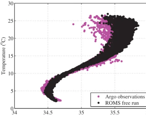
that the new atmospheric surface forcing is in balance with SST from BRAN3 for each month. To ensure that the higher-resolution atmospheric forcing did not significantly alter the previous model comparison, we integrated the model for two years without assimilation (hereafter referred to as the “2 yr free run”) and compared the model-derived SST with those from the advanced very-high-resolution radiome-ter (AVHRR) satellite data. The 2 yr free-run model spatially averaged SST and the spatially-averaged SST observations exhibit a small net bias over the 2012–2013 period (0.28◦). The temperature–salinity (T–S) diagram of data from Argo floats over the 2-year reanalysis period matches well with the correspondingT–S diagram for the 2 yr free-run output in-terpolated onto the Argo float locations and times (Fig. 4). This provides further confidence that the ROMS model con-figuration is capable of simulating the vertical structure of temperature and salinity in the region.
3.2 Data assimilation scheme
34 34.5 35 35.5 36 0
5 10 15 20 25 30
Salinity
Temperature (
o C)
Argo observations ROMS free run
Figure 4.Temperature–salinity diagram for the Argo observations and corresponding values from the 2 yr free run for 2012–2013.
should have the most complete description of the ocean state available. To accomplish this, we use IS4D-Var. IS4D-Var uses variational calculus to solve for increments in model initial conditions, boundary conditions, and forcing such that the difference between the modelled solution and all avail-able observations is minimised – in a least-squares sense – over the assimilation window. This is achieved by minimis-ing an objective cost function, J, that measures normalised deviations of the modelled ocean state from the observations as well as from the modelled background state (the model prior).
The forward integration of the nonlinear model equations, given a prior estimate of the initial conditions, surface, and boundary forcings, provides an estimate of the background state. The evolution of the state vector, x, for times t=
t1, . . ., ti−1, ti, . . ., tncan be written as
x(ti)=M(ti, ti−1)(x(ti−1),f(ti),b(ti)), (1)
whereMrepresents the nonlinear model equations operating onx(ti−1)and subject to forcingf(ti)and boundary
condi-tionsb(ti). The initial time for each data assimilation cycle is
denoted byt0and the model time step isti−ti−1. The goal of
the assimilation system is to generate a vector of increments that are added to the model initial conditions, boundary con-ditions, and forcing such that the quadratic cost function,
J, is minimised. The increments describe departures of the initial conditions, surface forcing, and open-boundary condi-tions from those applied to the model prior, such that x(t0)=xb(t0)+δx(t0), (2)
f(ti)=fb(ti)+δf(ti), (3)
b(ti)=bb(ti)+δb(ti), (4)
where xb(t
0) represents the background circulation initial
conditions andfb(ti)andbb(ti)are the background
circula-tion surface forcing and boundary condicircula-tions att=ti
respec-tively. Because the incrementsδx,δf andδbare assumed to be small relative to the background fields, they can be ap-proximately described by the linearised model equations, re-ferred to as the tangent-linear model. Utilising Bayesian in-ference and assuming Gaussian uncertainties in the observa-tions and model prior, we can formulate a cost function that is a function of the increment adjustments. Following Courtier (1997), we define the increment vector
δz=(δx(t0)T, δfT(t1), . . ., δfT(tn),
δbT(t1), . . ., δbT(tn))T, (5)
representing the increments to the initial conditions (timet0),
and the surface forcing and boundary conditions for model timest1totn. The cost function can then be written as J (δz)=1
2
n
X
i=0
(HiM(ti, t0)δz−di)TRi−1(HiM(ti, t0)δz−di)
+1 2(δz)
TP−1(δz)=J
o+Jb, (6)
whereM(ti, t0)represents the tangent-linear version of the
nonlinear model equationsM, integrated fromt0toti. The
difference between the modelled background state and the observations is represented by the innovation vector, given at each timeti bydi=yi−Hi(xb(ti)); whereyare the
ob-servations andHi is the linear operator that interpolates the
background circulation to observation points in space and time.Ris the observation error covariance matrix andPis the background error covariance matrix. The observation term of the cost function,Jo, represents the difference between the
model and the observations, and is obtained by the squared difference between the observations and the model given the integration of the increment adjustment through the tangent-linear model, weighted by the inverse of the observation error covariance.Jbis given by the squared increment, weighted
by the inverse of the background error covariance matrix, which describes the uncertainty in the initial conditions, sur-face, and boundary forcing.
The first step of the assimilation procedure is the forward integration of the nonlinear model equations to estimate the background state (referred to as the firstouterloop of the as-similation methodology), from which the initial cost function is computed. We seek to minimise the cost function by equat-ing the gradient to zero. The gradient of the cost function is given by
∇δzJ =
n
X
i=0
M(ti, t0)THTi R
−1
i (HiM(ti, t0)δz−di)
+P−1(δz), (7)
whereM(ti, t0)T is the adjoint of the tangent-linear model
is integrated using the increment δz (for the first iteration,
δz=0) and HiM(ti, t0)δz−di is computed. The adjoint
model is then used to compute the first term of Eq. (7) and∇δxJ is computed. A Lanczos-based conjugate gradient method is used to determine how far to step in the direction of the gradient to reduceJ and a new increment,δz, is gen-erated. Subsequent integrations of the tangent-linear and ad-joint models (referred to as theinnerloops) are continued to generate subsequent increments to minimiseJ. In practice, the inner loops can be continued untilJis reduced by a cer-tain ratio or, as in this study, a set number of inner loops can be completed that are found to give an acceptable reduction inJ. We do not find the true minimum ofJ, but rather an acceptable reduction. After the last inner loop, the final in-crement is applied to generate new initial conditions, bound-ary and surface forcing. The new integration of the nonlinear model, given the increment adjustments, completes the outer loop. The final outer loop provides the “best estimate” of the ocean state (the analysis), which is constrained to satisfy the nonlinear model equations (strong-constraint) and better rep-resent the observations over the assimilation window. The analysis provides an improved estimate of the initial state for the subsequent assimilation window.
An advantage of this assimilation method is that it makes use of the dynamical connections between the model fields, such that observed variables propagate information to unob-served, dynamically linked variables. Because the linearised model equations are used for the cost function minimisation, the length of the assimilation window is limited by the time over which the tangent-linear assumption remains reason-able. For a thorough description of the IS4D-Var formulation, the reader is referred to Moore et al. (2011c). The ROMS 4D-Var implementation is well described by (Moore et al., 2011c, a, b), and it has been used successfully in ROMS ap-plications (e.g. Di Lorenzo et al., 2007; Powell et al., 2008; Powell and Moore, 2008; Broquet et al., 2009; Matthews et al., 2012; Zavala-Garay et al., 2012; Janekovi´c et al., 2013; Souza et al., 2014).
3.3 Assimilation configuration
The goal of the assimilation is to combine an uncertain model with uncertain observations to generate a circulation estimate that has reduced uncertainty and better represents the obser-vations. To do this we solve for the nonlinear ocean solution that is dynamically consistent with the observations and is free within the uncertainties in the system. As such, specifi-cation of the prior model and observation uncertainties is im-portant. These uncertainties are prescribed in the background and observation error covariance matrices and are important scaling factors in the cost function, J (refer to Eq. 6). The specification of the background and observation error covari-ances is described in Sect. 3.4 and 3.5 below, and their con-sistencies checked in Sect. 4.1.
The minimisation ofJ is performed over a specified time window in a sequence of linear least-squares minimisations in the inner loops, and the nonlinear model trajectory is up-dated in the outer loops. Through experimentation, we found that one outer loop, with 14 inner loops, gives an accept-able reduction inJfor a reasonable computational cost. Cost function convergence is shown in Sect. 4.2. We aim for the longest time window available without nonlinearities grow-ing too large. Linearity experiments (not shown) indicated that for this model configuration, the linear assumption re-mains acceptable for typical perturbations over 5 days, so we chose that as our window size. We overlap the 5-day ilation windows by 1 day, such that each subsequent assim-ilation cycle is initialised 4 days after the start of the previ-ous 5-day cycle. The overlap allows us to produce a blended product, which is constructed as a post-processing step us-ing a weighted average of the overlappus-ing times from adja-cent assimilation windows to build a continuous signal. The blended product can then be used for dynamical analysis and further nesting.
The ROMS 4D-Var allows for controlling both the initial conditions and the time-varying atmospheric and boundary forcing. We adjust the atmospheric forcing every 12 h and the open-boundary conditions every 24 h. The heat flux is the dominant adjustment in the atmospheric forcing over most of the domain, with the wind adjustment dominating in the vicinity of the HF radar.
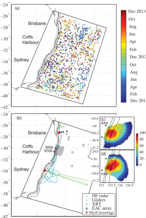
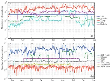
3.4 Observations and observation prior uncertainties The reanalysis time period (2012–2013) was chosen be-cause it contains the greatest number of available observa-tions, including a full-depth mooring array that resolves the EAC transport, which was deployed from 1 April 2012 to 26 August 2013. Other available subsurface observations and satellite-derived surface observations are also sourced for this time period. Figure 5a shows the location of Argo pro-filing float observations, coloured by time of occurrence, and Fig. 5b shows the location of all other observations, with the exception of the satellite-derived SSH, SST and sea surface salinity (SSS). The number of processed observations assimi-lated for each 5-day assimilation window is shown in Fig. 6a, with a break-down of the provenance of the temperature ob-servations in Fig. 6b. The obob-servations and their respective processing for assimilation into the reanalysis are detailed in the subsections below.
spa-Figure 5.Argo observations coloured by time of occurrence(a), and all other observations, with the exception of satellite-derived SSH and SST (b); 100, 200, and 2000 m contours are shown. Coastal towns are labelled in line with their location on the coast. HF radar sites Red Rock (RRK) and North Nambucca (NNB) are shown with black asterisks in (b)and insets showing the percent coverage of radial data for the two stations are shown in(c)and(d).
tial and temporal resolution of the model and the processes resolved. Observations that capture processes unresolved by the model must be either filtered or an uncertainty applied that accounts for the unresolved process. If multiple observa-tions from the same instrument exist in the same horizontal and vertical grid cell taken within the same model time-step (5 min), the observations are averaged and this value is as-similated within that grid cell at the appropriate time. The variance of those observations provides a lower-bound to the representation error as the model can express only a single value. Oftentimes, this error is greatest where the model reso-lution (and therefore its physics) cannot represent finer-scale dynamics captured in the observations. A thorough discus-sion of representation error can be found in Oke and Sakov (2008).
We describe the observations used in the section below, and detail the observation uncertainties specified for each. The consistency of these uncertainty estimates is checked in Sect. 4.1.
3.4.1 Satellite-derived sea surface height
AVISO, France, produce global, daily, gridded (1/4◦×1/4◦) mean SLA data produced by merging all available along-track satellite altimetry data, computed with respect to a 7-year mean. The AVISO data provide a daily statistical field giving a synoptic view of the SSH. The AVISO SLA data are added to the dynamic SSH mean from the 10 yr free run de-scribed above to generate sea level data for assimilation that are consistent with the ROMS model bathymetry and con-figuration. We prescribe an observation uncertainty of 6 cm. The error in the AVISO delayed-time global SLA product due to noise for the region is estimated at 2 cm (CNES, 2015). We include a further 4 cm of uncertainty because, in this case, the model resolves far more structure at smaller spatial scales than is capable in the observations. The AVISO fields pro-vide a statistical fit to along-track SSH data and the obser-vation uncertainty allows for imbalances between this sta-tistical field and a dynamically balanced SSH field required by the model. We exclude SSH observations that were taken over water depths less than 1000 m. This is because the ob-servations are noisy on the continental shelf and the AVISO gridded product is not able to resolve the processes that occur here.
The gridded AVISO product is used to constrain SSH, rather than the along-track altimetry, to ensure that the con-straint is projected into the baroclinic ocean state solution. The use of along-track SSH data successfully with 4D-Var relies on the prescription of balanced terms in the back-ground error covariance matrix to describe the covariance between SSH and the subsurface ocean (refer to Sect. 3.5). This is a topic of further research.
3.4.2 Satellite-derived Sea Surface Temperature We use SST from the US Naval Oceanographic Office Global Area Coverage Advanced Very High Resolution Radiometer level-2 product (NAVOCEANO GAC AVHRR L2P SST). The product does not provide observations through clouds but contains useful observations close to the coast. Data are available 2–3 times per day. A product error is specified in the NAVOOCEANO SST product (Andreu-Burillo et al., 2010), with an error for each data point of 0.38–0.4◦C. As the
res-olution of the data is similar to the resres-olution of the model, the observation uncertainty for the assimilation is chosen to be equal to this product error.
3.4.3 Satellite-derived sea surface salinity
Jan Apr Jul Oct Jan Apr Jul Oct Jan
101
102
103
104
105
Number of observations
SSH and Temp. Salt Radials
(a)
Jan Apr Jul Oct Jan Apr Jul Oct Jan
101
102
103
104
105
Number of obsservations
SST NAVO Gliders Argo XBT
SEQ moorings NSW moorings EAC array
(b)
-u v
Figure 6.Number of observations (after processing) used in each 5-day assimilation window; for each observation type(a), and temperature observations for each data source(b).
Aquarius satellite (www.aquarius.umaine.edu/). We make use of the level 3 gridded salinity product, which provides daily fields at a 1◦ resolution. The observation uncertainty is set to 0.4. There is a product error of around 0.2 for the Aquarius SSS data and 0.4 is chosen to account for addi-tional uncertainty due to processes not resolved by the obser-vations or the model. The value is considerably higher than the uncertainties specified for other in situ salinity observa-tions. Similarly to SSH, any data taken over water depths less than 1000 m depth were eliminated.
3.4.4 Argo floats
Argo is an international program consisting of nearly 4000 free-drifting profiling floats that measure the temperature and salinity of the upper 2000 m of the global ocean (www.argo. ucsd.edu). The Argo float locations in our model domain for 2011–2012, and the times at which they occur at those loca-tions, are shown in Fig. 5a. The Argo data points are averaged to the model grid and a 5 min time step.
Uncertainty profiles are defined to specify the nominal minimal uncertainties for subsurface temperature and salin-ity. To devise the profile shapes, temperature and salinity variance is computed for each month of the year from the 10 yr free run. The monthly variances are spatially averaged over the model domain and averaged in time to give a single variance profile for both temperature and salinity. The pro-files are then scaled to provide variance propro-files appropriate
for the nominal minimum observation error variance, based on preliminary assimilations and checks against the diagnos-tics described in Sect. 4.1 (computed throughout the water column). The uncertainty profiles are shown in Fig. 7 (stan-dard deviation is plotted instead of variance so the units are more intuitive for the reader). The profiles provide greater uncertainties in the depth ranges of the greatest variability, where representation errors are likely to be the largest. The observation error variance is specified as the maximum of this nominal minimum error variance and the variance of the observations from the same model cell.
3.4.5 Expendable Bathythermographs
0 0.1 0.2 0.3 0.4 0.5 0.6 0.7
ï ï ï ï ï ï ï ï ï ï
0
Temperature standard deviation (oC)
Depth (m)
0 0.05 0.1 0.15 Salinity standard deviation
Figure 7.Nominal minimum observation uncertainty profiles ap-plied to subsurface temperature and salinity observations offshore of the continental shelf.
(Fig. 7) is used and the observation error variance is specified as the maximum of the nominal minimum error variance and the variance of the observations from the same model cell. 3.4.6 High-frequency radar
The Coffs Harbour high-frequency (HF) ocean radar is part of the IMOS and is managed by the Australian Coastal Ocean Radar Network (ACORN; http://imos.org.au/acorn. html). The radar is a WERA phased-array system with 16-element receive arrays located at Red Rock (RRK; 29.98◦S,
153.23◦E) to the north of Coffs Harbour and North
Nam-bucca (NNB; 30.62◦S, 153.011◦E) to the south. The radars operate at a frequency of 13.920 MHz, with a bandwidth of 100 KHz and a maximum range of 100 km.
The HF radar broadcasts and receives along defined an-gles in a phased-array set-up and the surface current speed (towards and away from the radar site) is measured. The overlapping coverage from the two radar sites allows for the surface current (uandv) vectors to be computed. Using the same assimilation procedure as detailed in Souza et al. (2014), we assimilate radial currents, rather than the com-puted current velocities. The velocities have correlated er-rors and using the radials allows us to make use of data when only one station is available and over areas that do not over-lap with the other station’s measurements. We can also make use of radial data in regions where the beam intersection an-gle between measurements from the two stations results in a high error in the velocity calculation, whereas the radials errors are adequately low.
Radial data are available from 1 March 2012 to the end of the reanalysis period. The areas of HF radar coverage are shown in Fig. 5b, with inset panels showing the percentage of data coverage for assimilated radials for the RRK and NNB
sites in Fig. 5c and d respectively. Radials for each of the two stations are processed separately. At the outer range of the HF radar instrument coverage, radial values become noisy. We extract only radial values with a Bragg signal-to-noise ra-tio>10 dB. Manual inspection of the radial values for each of the two sites was then conducted and a “good data” re-gion was chosen for each site every day, excluding the outer regions of coverage where noisy data are observed. Only ra-dial data within these “good data” regions is used, and ab-solute radial speed values greater than 2 ms−1are excluded. This manual inspection was performed daily as the radii of reliable radial data vary significantly, and this method allows us to retain the maximum amount of data for assimilation. The radial speeds and angles are spatially averaged onto the model grid and a 24 h boxcar-averaging filter is used to re-move tides and inertial oscillations that are not resolved by the model.
Radial speed standard error is given in the data files pro-vided by ACORN, calculated from the mean width of the two Bragg peaks weighted by their maximum power (Wy-att, 2014). These standard errors are converted to variances and averaged as above. An error variance is then applied to each observation, given by the maximum of the averaged variances and the variance of the averaged radial speeds. The nominal minimum observation error for the surface ra-dials is set to 0.15 ms−1. The observation error covariance for each radial speed observation is set to the maximum of the nominal minimum observation error covariance and the error variance computed during the averaging. Any observa-tions where the square-root of the radial speed error variance exceeds the radial speed magnitude are removed. Radial data within one grid cell of the coast are also removed as unreal-istically high values are observed here.
3.4.7 NSW shelf moorings
Data collected from three moorings located along the NSW continental shelf are used in this assimilation study. The moorings collect temperature and velocity data at high sam-pling frequencies and are located off the coast of Coffs Harbour, 30◦S (CH100) and Sydney, 33.9◦S (SYD100 and SYD140). In each case the number in the mooring name rep-resents the approximate water depth of the mooring loca-tion. Table 2 contains details of the mooring locations and the properties observed. Temperature and velocity observa-tions are every 8 m through the water column. The data col-lection and quality control is described in detail in Roughan and Morris (2011).
Table 2.Mooring information for the EAC deep water array moorings (EAC1-5), South East Queensland shelf moorings (SEQ200, SEQ400) and the NSW shelf moorings (CH100, SYD100, SYD140).
Sensor depth range (m)
Name Lat Long Water Distance Temporal Temperature Salinity Velocity
(◦S) (◦E) depth (m) offshore (km) coverage
CH100 30.27 153.40 98 25 1 Jan 2012–30 Dec 2013 5–100 – 9–89
SYD100 33.94 151.38 104 10 1 Jan 2012–30 Dec 2013 11–107 – 1–99
SYD140 33.99 151.45 138 19 1 Jan 2012–30 Dec 2013 21–143 – 24–129
EAC1 27.31 153.97 1525 53 21 Apr 2012–23 Aug 2013 60–1060 60–1060 43–1054
EAC2 27.31 153.99 1940 55 22 Apr 2012–24 Aug 2013 163–1045 163–1045 9–1495
EAC3 27.25 154.29 4220 85 23 Apr 2012–24 Aug 2013 156–3991 156–3991 9–3968
EAC4 27.21 154.65 4745 121 25 Apr 2012–25 Aug 2013 154–4009 154–4009 38–3974
EAC5 27.10 155.30 4797 185 26 Apr 2012–26 Aug 2013 192–1109 192–1109 107–4016
SEQ400 27.33 153.88 405 44 1 Apr 2012–6 Jun 2013 48–375 48–375 23–405
SEQ200 27.34 153.77 209 33 1 Apr 2012–6 Jun 2013 40–189 40–189 23–196
diurnal surface heating for near-surface temperature observa-tions. The rms residual between the mooring temperature ob-servations low-pass filtered at 30 h (removing variability due to baroclinic tides and inertial oscillations) and the observa-tions filtered at the inertial frequency is very small compared to the nominal minimum uncertainties applied, confirming that these unresolved processes are accounted for in the ob-servation uncertainty specification. Velocity obob-servations are low-pass filtered at 30 h to remove variability due to tides and inertial oscillations and applied 6 hourly. It is important to remove the tidal signal from velocity observations as the barotropic tidal velocities are of a similar order of magnitude to the sub-tidal velocities.
For all observations on the continental shelf, different nominal minimum observation error variance profiles are adopted (to those used offshore for Argo and XBT) to ac-count for increased variability due to finer-scale processes that occur on the shelf that are not resolved in the model. Variance profiles for the shelf observations were computed by comparing all of the shelf observations (NSW moorings, SEQ moorings, and gliders) to the 2 yr free run for the 2012– 2013 assimilation period to generate a nominal uncertainty profile on the shelf. Profiles were generated for all observed in situ variables:uandvvelocity components, temperature, and salinity.u(v)uncertainty peaks at 0.12 (0.3) ms−1in the upper 50 m reducing to 0.08 (0.1) ms−1at 200 m depth. The shelf temperature uncertainty profile peaks at 1.2◦C between 20–100 m depth, reducing to 0.8◦C at 200 m. We doubled the computed salinity errors to give a range of 0.1–0.16 for the upper 200 m on the shelf.
The observation error variance is specified as the maxi-mum of the nominal minimaxi-mum error variance and the vari-ance from averaging observations within the same model grid cell. For velocities, the high density of the ADCP depth bins means several velocity measurements are often available for
a single vertical grid layer, which can result in variances that exceed the specified nominal minimum uncertainty.
3.4.8 EAC transport array and SEQ shelf moorings The EAC transport array was deployed as part of IMOS to understand the variability of the EAC, and it is comprised of five deep water moorings (EAC 1–5), which measure tem-perature, salinity, and velocities. The array was positioned where the EAC is predicted to be most coherent and was de-signed to measure the mean and time-varying EAC transport (Sloyan et al., 2016). The array is continued onto the shelf slope and shelf with two moorings (SEQ400 and SEQ200) in approximate water depths of 400 and 200 m respectively. Each mooring has a suite of instruments measuring temper-ature, salinity, and velocities at high sampling frequencies throughout the water column. Table 2 contains details of the moorings.
3.4.9 Ocean gliders
Autonomous ocean gliders (both SeaGliders and Slocum) were deployed as part of the IMOS by the Australian Na-tional Facility for Ocean Gliders (http://imos.org.au/anfog. html). The buoyancy controlled gliders move horizontally through the water while collecting vertical profiles of temper-ature and salinity. The majority of the glider missions in the model domain over the 2011–2012 time period occur on the NSW continental shelf, between 29.5 and 32.3◦S, with two missions between 25 March and 22 July 2013 extending off-shore, further south, and to depths of 900 m (Fig. 5b). Quality control flags are applied to the glider data through the IMOS processing (Australian National Facility for Ocean Gliders, 2012) and only the data deemed to be “top quality data in which no malfunctions have been identified and all real fea-tures have been verified during the quality control process” are used. The glider data points are averaged onto the model grid and a 5 min time step. Glider temperature data in the up-per 20 m and salinity data in the upup-per 50 m were removed. The uncertainty profiles computed for the shelf observations were used and the error variances for the gliders are the maxi-mum between the variance computed from the averaging and the shelf error variance profile.
3.5 Model prior uncertainties
The background error covariance matrix,P, should represent the expected uncertainties in the model initial conditions, sur-face, and boundary forcings.Pis anMbyMmatrix, where
M is the length of the increment vectorδz(Eq. 5). Because of its size Pcannot be estimated completely or stored and we estimate Pby factorisation, as described in Weaver and Courtier (2001), such that
P=Kb63L1v/2LhL1v/236KTb, (8)
whereKbare the covariance operators of the balanced
dy-namics,6and3are the diagonal matrices of the background error standard deviations and normalisation factors respec-tively, and Lv andLh are the univariate correlations in the
vertical and horizontal directions. In this work, we only pre-scribe univariate covariance in Kb. The dynamics are
cou-pled through the use of the tangent-linear and adjoint models in the assimilation, but not in the statistics of P. The corre-lation matrices,LvandLh, and the normalisation factors,3,
are computed as solutions to diffusion equations following Weaver and Courtier (2001). The characteristic length scales chosen forLvandLhare assumed to be homogeneous and
isotropic.
In the horizontal, the characteristic length scales chosen for the background error covariances are 100 km for SSH, temperature, and salinity, and 70 km for velocities. These val-ues were chosen based on analysis of cross-correlation of SSH and complex correlation of surface velocities between points in the eddy rich Tasman Sea region from the 2 yr free
run. The length scale of 100 km for SSH is consistent with the decorrelation scales estimated from along-track satellite data for the area by Wilkin et al. (2002) and used by Zavala-Garay et al. (2012). It is noted that shorter cross-shore length scales are likely along the coast of south-eastern Australia, as the continental shelf is narrow (15–30 km) and the EAC displays a narrow jet-like structure, while SSH decorrelation length scales were found to be about 100–200 km in the alongshore direction by Oke and Sakov (2012).
For the vertical, semivariogram analysis of glider data on the NSW shelf by Schaeffer et al. (2016) found vertical decorrelation length scales of about 50 m for both tempera-ture and salinity on the NSW shelf. Analysis of correlations between temperature data measured by the moorings used in this study found vertical decorrelation length scales of 15– 30 m for the shelf moorings (NSW moorings, SEQ 200), 70 m for SEQ 400, and 100–200 m for the EAC deepwa-ter array moorings (EAC 1–5). Salinity measurements were taken at SEQ200, SEQ400, and the EAC deep water array moorings and decorrelation length scales were similar to the length scales for temperature at these moorings. In the verti-cal, we apply characteristic length scales of 50 m for salinity and 10 m for temperature. The shorter length scale for tem-perature was adopted due to the short length scale of variabil-ity for temperature near the sea surface, as SST observations dominate. The salinity length scale is set to 50 m (longer than the temperature length scale) in order to limit vertical struc-ture in the salinity analysis increments.
Analysis of correlations between velocities measured by the moorings found vertical decorrelation length scales of 20–50 m for the shelf moorings (NSW moorings, SEQ 200), 70 m for SEQ 400, and 100–200 m for the EAC deep water array moorings (EAC 1–5). Because the deep water moor-ings span the core of the EAC, we reduced the de-correlation length scale value to 50 m in the vertical for velocity to en-sure consistency when assimilating velocities outside of the EAC and/or on the shelf.
The background error covariance matrix plays an impor-tant role in determining the spatial structure of the analysis increment and, in this oceanic region, the horizontal and ver-tical scales of variability differ between the mesoscale eddy field in the Tasman Sea and the smaller-scale shelf processes. Further research on the impact of applying anisotropic corre-lation length scales on system performance is warranted.
0 0.4 0.8 1.2 1.6 2
Jan Apr Jul Oct Jan Apr Jul Oct
Cost function
(a)
5-day assimilation cycles x 105
J initial Final NLM J Final TLM J (b)
0 1 2 3 4 5 6 7 8 9 10 11 12 13 14 0.2
0.4 0.6 0.8 1
Inner loops
TLM J / Initial J
J TLM reduction Final J NLM reduction
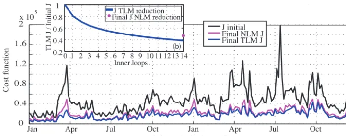
Figure 8.Initial nonlinear cost function and the reduction achieved in the final (14th) tangent-linear modelinner loopand the final nonlinear cost function, plotted for each assimilation interval(a). Mean cost function reduction for each of the 14 inner loops for all 5-day assimilation intervals(b).
occur over 5 days. The same background error covariance matrix is used for each assimilation cycle.
4 Reanalysis evaluation
In this section, we evaluate the performance of the assimi-lation procedure in terms of the consistency of the prior un-certainty assumptions, comparison with the assimilated ob-servations, and comparison to unassimilated observations. Overall, the assimilation performs well in minimising the cost function over each assimilation interval and the corre-sponding reanalysis provides a good match to observations. 4.1 Consistency of observation and model uncertainties The analysis generated by the IS4D-Var system is dependent on the prior assumptions of the background and observa-tion uncertainties, and the validity of these assumpobserva-tions is important in determining the optimality of the analysis. A measure of the consistency of the assimilation system given the prior uncertainty assumptions can be made using a set of diagnostics based on the innovation statistics, presented in Desroziers et al. (2005). These diagnostics are based on the observation minus background, observation minus anal-ysis, and analysis minus background differences and provide a check of the consistency of the prior choices of the back-ground and observation error covariances. The level of agree-ment between the a priori specified error variances (PandR), and those diagnosed a posteriori following the methods intro-duced by Desroziers et al. (2005) provides a measure of the appropriateness of the estimates ofPandR. We find that the prior specified error variances and those diagnosed after the assimilation match well.
For SSH, square-root of the spatially averaged diagnosed observation error variance ranges from 4.1 to 8.4 cm with a mean value of 5.8 cm, which matches the square root of the prior observation error variance of 6 cm very well. The
SSH prior and diagnosed model error variances are also con-sistent. For subsurface temperature, the prior and diagnosed model error variances match very well. The prior observation error variances are greater than the diagnosed observation er-ror variances for subsurface temperature; the time mean of the square root of the spatially averaged prior error variances is 0.88◦C compared to 0.48◦C for the diagnosed errors. This prior uncertainty was necessary to account for the representa-tion errors associated with the subsurface temperature obser-vations. Similarly for subsurface salinity and velocities, the prior observation error variances exceed the diagnosed obser-vation error variances. For the radial current speeds, the time mean of the square root of the spatially averaged diagnosed observation error variances is 0.11 ms−1, which matches the prior observation uncertainty of 0.15 ms−1well.
Another simple diagnostic to check the validity ofPandR is to check the value of the cost function,J, at its minimum. As shown by Bennett (2002), the theoretical minimum of the cost function, for a linear system, isNobs/2, whereNobsis the
number of observations. This minimum should be reached on each assimilation cycle if the prior background and obser-vation error covariance estimates are correctly specified and the system is quasi-linear (Weaver et al., 2003). It is conve-nient to define the “optimality” value,γ=2J /Nobs, which
should reach a value of 1±√2/Nobs(Powell et al., 2008).
AsNobsis large, a value of 1 indicates correct specification
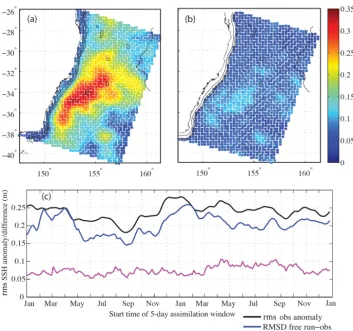
Figure 9.The rms SSH observation anomaly(a)and rms SSH difference between the analysis and observations(b)for the 2-year assimilation window. Time series of spatially averaged rms SSH observation anomaly, rms SSH difference between the free run and observations, and rms SSH difference between the analysis and observations, for each assimilation window(c).
4.2 Cost function reduction and convergence properties
Linear minimisation of the cost function,J, is performed in the inner loops. We use a single outer loop, at the end of which the final cost function is computed after the integration of the nonlinear model. Figure 8a shows the initial nonlin-ear cost function (black), the reduction achieved in the final (14th) inner loop (blue), and the final nonlinear cost function (magenta), plotted for each assimilation interval over the 2-year period. The match between the final tangent-linear and the nonlinear cost functions provides confidence in the valid-ity of the tangent-linear assumption over the 5-day assimila-tion window. The mean tangent-linear model cost funcassimila-tion reduction (1−JTLM/Jinitial, where JTLM is the cost
func-tion for the final inner loop) over all assimilafunc-tion windows is 62 %, and the mean of the subsequent nonlinear model cost function reduction (1−JNLM/Jinitial) is 52 %. Temperature
dominates the cost function, followed by the velocities (in-cluding the radials) and SSH, with salinity playing the least dominant role. Figure 8b shows the mean cost function re-duction for each of the 14 inner loops for all 5-day
assim-ilation windows. The cost function reduction relative to the initial cost function increases with each inner loop, and the curve begins to flatten out towards the final inner loop show-ing that 14 loops is a good choice. The mean reduction in the nonlinear cost function is shown by a magenta dot in the plot and shows that minor nonlinearities persist in our assimila-tion windows.
4.3 Reanalysis comparison to assimilated observations 4.3.1 SSH
Figure 10.The rms SST observation anomaly, including seasonal cycle,(a)and rms SST difference between the analysis and observations (b)for the 2-year assimilation window. Time series of spatially averaged rms SST observation anomaly, rms SSH difference between the free run and observations, and rms SSH difference between the analysis and observations, for each assimilation window(c).
The observation anomaly for an observed variable v at a particular location is given by
rmsObsAnom= s
6tn
t1(v(t )−v) 2
n , (9)
wheret=t1, t2, . . .tn are the observation times andv is the
time mean of the observed variable at that location. The rms difference between the free-run values (in observation space) and the observations and the analysis and observations are given by
RMSDFreerun−Obs= s
6tn
t1(vf(t )−vo(t )) 2
n , (10)
and
RMSDAnalysis−Obs= s
6tn
t1(va(t )−vo(t )) 2
n (11)
respectively, wherevois the observed value,vfis the
corre-sponding value from the free run, andvais the corresponding
value from the analysis.
Figure 9a shows the rms SSH anomaly from the observations over the 2-year assimilation period. The RMSDAnalysis−Obs is shown in Fig. 9b and shows that the
SSH fields are well represented in the analyses. In Fig. 9c, the domain-averaged rmsObsAnom, RMSDFreerun−Obs, and
RMSDAnalysis−Obs are plotted for each 5-day assimilation
window over the 2-year period, showing significant im-provement in the fit to observations in the analyses. The RMSDFreerun−Obs is of similar magnitude to the SSH
ob-servation anomaly indicating that, as expected, the free run has no skill in predicting the timing and location of the mesoscale eddies. The time mean of the spatially averaged RMSDAnalysis−Obs over all assimilation windows is 7.6 cm.
This is close to the observation uncertainty for SSH of 6 cm and small compared to the typical SSH variability (the time mean of the spatially averaged SSH observation anomalies is 23.4 cm).
4.3.2 SST
RMSD temperature ( C)o
Depth (m)
Argo XBT Gliders
0 1 2 3 4 5
0 1 2 3 4 5 0 1 2 3 4 5
ï ï ï ï ï ï ï ï ï ï
0
RMSD analysis - obs RMSD freerun - obs
RMSD freerun - bias adjusted obs
Figure 11.The rms difference between the free run and observations, the free run and the bias-adjusted observations, and the analysis and observations for Argo(a), XBT(b), and glider(c)observations in nominal depth bins for the 2-year assimilation window. Argo and XBT depth bins are 25 m from the surface to 200 and 50 m below 200 m, glider bins are 10 m throughout the water column.
ever, significant improvement is achieved in the analyses. The rms SST observation anomalies describe the variabil-ity in SST over the 2-year assimilation period, includ-ing the seasonal cycle, and are shown in Fig. 10a. The RMSDFreerun−Obs is smaller than the observation
anoma-lies and the RMSDAnalysis−Obs (Fig. 10b) is further
re-duced. The time series of spatially averaged rmsObsAnom,
RMSDFreerun−Obs and RMSDAnalysis−Obs are shown in
Fig. 10c over the 2-year period. The time mean of the spa-tially averaged analysis error for all assimilation windows is 0.4◦C, which is the same magnitude as the SST vation uncertainty. The free-running model and SST obser-vations exhibit no net bias over the 2 years (as mentioned in Sect. 3.1), indicating that the RMSD reduction between the free run and the analysis is due to improved prediction of the dynamical features rather than a reduction in bias. The high variability seen in the time-series plots, particularly in the observation anomaly, is due to the patchy spatial coverage of the SST observations.
4.3.3 SSS
The Aquarius SSS data were included but for this assimila-tion configuraassimila-tion provides little constraint. The rmsObsAnom
for SSS is 0.15–0.3 over most of the model domain (up to 0.5 at a few points close to the coast). The Aquarius product error itself is 0.2 and our specified observation error is 0.4,
which is greater than the typical variability in SSS over most of the domain, so the assimilation does little to match the SSS observations as they are so uncertain. The RMSDFreerun−Obs,
RMSDAnalysis−Obs, and rmsObsAnomare all of similar
magni-tude. Subsurface salinity dominates the salinity cost function as the prescribed observation uncertainties are considerably higher for SSS than the uncertainties specified for the in situ salinity observations.
4.3.4 Subsurface temperature from Argo, gliders and XBT
Subsurface observations are spatially and/or temporally sparse in comparison to satellite observations of the sea surface. The dynamical connections between surface and subsurface variables are taken into account by the adjoint and tangent-linear model such that the time-evolving model physics are used to perform the cost function minimisation. While these connections allow for the surface observations to impact state estimates of the subsurface properties, sub-surface observations are invaluable in improving estimates of the subsurface (e.g. Zavala-Garay et al., 2012).
We show the improvement in subsurface temperature as measured by the Argo floats, XBTs and ocean gliders by computing the RMSDFreerun−Obs and RMSDAnalysis−Obs in
0 0.1 0.2 0.3 0.4 0.5 0.6 0.7 0.8 0
rms potential density anomaly/difference (kg m )-3
Depth (m)
rms obs. anomaly RMSD free run -obs RMSD analysis - obs
Figure 12.The rms potential density observation anomaly and rms difference between the free run and observations, and the analy-sis and observations for Argo float observations. Observations are grouped into nominal depth bins of 25 mm from the surface to 200 and 50 m below 200 m.
all observations in the upper 500 m of the water column is 1.7◦C, reduced to 0.8◦C in the analysis. For the XBT above
500 m, the time-mean RMSD is reduced to 0.7◦C in the anal-ysis from 1.9◦C for the free-running model. Below 500 m, the number of observations in each depth bin for Argo and XBT is too low for a meaningful comparison. The glider data mostly samples the shelf and shelf slope circulation. A great majority of the glider observations are in the upper 100 m of the water column; here the time-mean RMSDFreerun−Obs of
2.1◦C is reduced to 0.7◦C in the analysis.
To investigate the relative contribution of improved repre-sentation of dynamical features and reduction in bias to the RMSD reduction between the free run and the analysis, we also compute the RMSD between the free run and the “bias-adjusted observations”. The bias-“bias-adjusted observations have the bias between the observations and the free run removed and, for each depth bin, are given byvo(t )−(vo−vf), where vois the observations in the depth bin for observation times t=t1, t2, . . .tn,vf is the corresponding values from the free
run and the overbar represents the time mean of the variables over the 2-year period. For the Argo and XBT observations, the bias between the free run and the observations is small and the RMSDFreerun−Obs and the RMSD between the free
run and the bias-adjusted observations (blue and grey dashed
lines in Fig. 11 respectively) match closely. The RMSD re-duction for the analysis (magenta line) is due to better rep-resentation of the dynamical features. The vast majority of glider observations are taken on the continental shelf in water depths less than 100 m. For these shallow glider observations, the bias between the free run and the observations is approxi-mately 1.5◦C (not shown). The bias in the analysis is close to zero and this reduction in bias contributes to the reduction in the RMSDAnalysis−Obs compared to the free run (the RMSD
between the free run and the bias-adjusted observations (grey dashed line) is less than the RMSDFreerun−Obs (blue line)).
There is further reduction in the RMSDAnalysis−Obs(magenta
line) compared to the RMSD between the free run and the bias-adjusted observations (grey dashed line) indicating im-proved representation of dynamical features. It should be noted that the glider observations below 100 m represent only two separate glider missions (refer to Sect. 3.4.9), so the bias has little meaning over this depth range.
As the Argo profiling floats measure both temperature and salinity at each observation time we are able to assess the residual reduction in terms of potential density through-out the water column (Fig. 12), describing the improvement in the representation of the density structure in the analy-sis. The free-running model has some skill in predicting po-tential density as sampled by the Argo floats in the upper 500 m, as the RMSDFreerun−Obs is less than the rmsObsAnom
for the nominal depth bins. The RMSDAnalysis−Obsin
poten-tial density is reduced to about half of the RMSDFreerun−Obs
in the upper 500 m; the upper layer that is most effected by mesoscale eddies. The RMSDAnalysis−Obsin potential density
peaks in the upper 100 m at 0.23 kg m−3and decreases grad-ually to below 0.1 kg m−3at 500 m depth, remaining below
that for the Argo-observed ocean deeper than 500 m. 4.3.5 Velocities from moorings
Complex correlation
Depth (m)
Complex correlation
Complex correlation Complex correlation Complex correlation
Depth (m)
Complex correlation Complex correlation
Complex correlation Complex correlation Complex correlation SEQ200m
EAC1
SEQ400m
EAC5 EAC4
EAC3 EAC2
CH100m SYD100m SYD140m
Free run, obs Analysis, obs
Figure 13.Complex correlation between observed velocities and free-run and analysis velocities at mooring locations.
mooring (CH100), 0.37 and 0.84 for the Sydney mooring (SYD100), and 0.36 and 0.87 for the other Sydney mooring (SYD140).
4.3.6 Surface velocities from HF radar
Here we choose to present the results in terms of surface velocities (rather than the scalar radial current speeds) as they are more meaningful in terms of the ocean surface cur-rents. The observed surface velocities are computed from the assimilated radials and the corresponding values com-puted from the radial values extracted from the free-running model and the analyses. The complex correlations between
Complex correlation coeffificient
0 0.1 0.2 0.3 0.4 0.5 0.6 0.7 0.8 0.9 1 2000
200
RRK
NNB
152.8 153.2 153.6 154 154.4
200 1000
RRK
NNB
152.8 153.2 153.6 154 154.4
2000 200 1000
-30
-30.5
-31
o o
o
o
o o o o o o o o o
Figure 14.Complex correlation of surface velocities computed from the assimilated HF radar radials, and surface velocities computed from the corresponding free run(a)and analysis(b)radials; 200, 1000, and 2000 m bathymetry contours are shown.
shelf and shelf slope with complex correlations reducing off-shore of the shelf slope. Velocity is very well represented in the analysis under the HF radar footprint, with complex cor-relations from 0.8–1 across the entire footprint.
In terms of the radial current speeds measured from both NNB and RRK sites, the RMSDFreerun−Obs is 0.1–0.4 ms−1
inshore of the 200 m depth contour, 0.2–0.6 ms−1above the shelf slope (between the 200 and 2000 m depth contours), and 0.3–0.5 ms−1offshore of the 2000 m depth contour. The RMSDAnalysis−Obs, for both NNB and RRK sites, is between
0.1 and 0.25 ms−1across the entire radar footprints. The ratio
of RMSDFreerun−Obs/rmsObsAnom is 0.5–1, reduced to 0.2–
0.5 for the ratio of the RMSDAnalysis−Obs/rmsObsAnom.
4.4 Reanalysis comparison to independent observations
Because IS4D-Var uses the model dynamics to solve for the increment adjustments, information from observed variables can propagate to unobserved regions such that the ocean state better fits and is in balance with the observations. Compari-son of the reanalysis with independent, non-assimilated, ob-servations allows us to assess the performance of the state estimate away from assimilated observations. As the princi-pal aim of this work was to assimilate the maximum number of available observations in the region in order to provide a “best estimate” of the ocean state over the 2-year period, few independent observations remain available for this compari-son.
The available independent observations are from ship-board conductivity–temperature–depth (CTD) casts that were taken on three separate cruises within the model domain over the 2-year period; 15 CTD casts were taken as part of the deployment of the EAC array, along the EAC array tran-sect from 21 to 27 April 2012 (blue diamonds in Fig. 15b). Five casts were taken off of Sydney between 34.3–36.4◦S and 151.6–152.8◦E from 27 to 28 February 2013 (magenta diamonds in Fig. 15b); 28 CTD casts were taken in two
tran-sects off of Brisbane at 26.3 and 27.1◦S out to 155.8◦E be-tween 21 and 31 August 2013 (green diamonds in Fig. 15b). The CTD cast observations are mapped to the model verti-cal levels for consistent comparison given the vertiverti-cal dis-cretisation of the model, and the corresponding model val-ues extracted from the 2 yr free run and the analysis. The rmsObsAnom, RMSDFreerun−Obs, and RMSDAnalysis−Obs for
potential density in nominal depth bins for all CTD casts are shown in Fig. 15a. In the upper 350 m of the water col-umn, the RMSDAnalysis−Obs in the potential density is
re-duced to about half of RMSDFreerun−Obs. For all CTD casts
in the upper 200 m, where the number of observations is the greatest (not shown), the depth-averaged RMSDFreerun−Obs
of 0.33 kg m−3 is reduced to 0.17 kg m−3 in the analysis. This shows that a marked improvement in the representation of the subsurface ocean, as observed by these CTD casts, is achieved in the reanalysis.
Note that the profiles of Argo RMSDFreerun−Obs and
RMSDAnalysis−Obs in potential density (Fig. 12) are similar
to the RMSD profiles for the independent shipboard CTD observations. The reanalysis showing similar residual reduc-tion for the assimilated Argo observareduc-tions and for the non-assimilated CTD cast observations suggests a well-specified assimilation system in which a dynamically balanced ocean state estimate is achieved with improved state-estimation throughout the model domain, rather than over-fitting to as-similated observations.
5 Summary and conclusions