www.geosci-model-dev.net/9/3875/2016/ doi:10.5194/gmd-9-3875-2016
© Author(s) 2016. CC Attribution 3.0 License.
Size-resolved simulations of the aerosol inorganic composition with
the new hybrid dissolution solver HyDiS-1.0: description, evaluation
and first global modelling results
François Benduhn1, Graham W. Mann1,2, Kirsty J. Pringle1, David O. Topping3, Gordon McFiggans3, and Kenneth S. Carslaw1
1School of Earth and Environment, University of Leeds, Leeds, UK
2National Centre for Atmospheric Science, School of Earth and Environment, University of Leeds, Leeds, UK
3Centre for Atmospheric Science, School of Earth, Atmospheric and Environmental Science, The University of Manchester,
Manchester, UK
Correspondence to:François Benduhn ([email protected])
Received: 30 November 2015 – Published in Geosci. Model Dev. Discuss.: 17 February 2016 Revised: 5 October 2016 – Accepted: 7 October 2016 – Published: 1 November 2016
Abstract. The dissolution of semi-volatile inorganic gases such as ammonia and nitric acid into the aerosol aqueous phase has an important influence on the composition, hy-groscopic properties, and size distribution of atmospheric aerosol particles. The representation of dissolution in global models is challenging due to inherent issues of numerical sta-bility and computational expense. For this reason, simplified approaches are often taken, with many models treating dis-solution as an equilibrium process. In this paper we describe the new dissolution solver HyDiS-1.0, which was developed for the global size-resolved simulation of aerosol inorganic composition. The solver applies a hybrid approach, which al-lows for some particle size classes to establish instantaneous gas-particle equilibrium, whereas others are treated time de-pendently (or dynamically). Numerical accuracy at a compet-itive computational expense is achieved by using several tai-lored numerical formalisms and decision criteria, such as for the time- and size-dependent choice between the equilibrium and dynamic approaches. The new hybrid solver is shown to have numerical stability across a wide range of numeri-cal stiffness conditions encountered within the atmosphere. For ammonia and nitric acid, HyDiS-1.0 is found to be in excellent agreement with a fully dynamic benchmark solver. In the presence of sea salt aerosol, a somewhat larger bias is found under highly polluted conditions if hydrochloric acid is represented as a third semi-volatile species. We present first results of the solver’s implementation into a global aerosol
microphysics and chemistry transport model. We find that (1) the new solver predicts surface concentrations of nitrate and ammonium in reasonable agreement with observations over Europe, the USA, and East Asia, (2) models that as-sume gas-particle equilibrium will not capture the partition-ing of nitric acid and ammonia into Aitken-mode-sized parti-cles, and thus may be missing an important pathway through which secondary particles may grow to radiation- and cloud-interacting size, and (3) the new hybrid solver’s computa-tional expense is modest, at around 10 % of total computation time in these simulations.
1 Introduction
The inorganic composition of the aqueous phase of atmo-spheric aerosol particles is continuously subject to exchange with the gas phase. Whereas H2SO4condenses irreversibly
under tropospheric conditions, semi-volatile species such as H2O, HNO3, HCl, and NH3 may re-evaporate from the
aerosol aqueous phase depending on the temperature and chemical composition of the atmosphere. NH3 combines
with H2O to give NH4OH, which along with HNO3and HCl
The dissolution of semi-volatile gases into the aerosol phase has an ambiguous effect on aerosol particle size. The dissolution of NH3within acidic H2SO4particles decreases
their hygroscopicity, resulting in a decrease in water content and particle size, while chemical interaction between a dis-solving acid and a disdis-solving base, such as HNO3and NH3,
may result in a substantial increase in particle size due to the considerable amount of dissolved matter and water that is bound by it. Variations in particle size and hygroscopicity affect aerosol–radiation and aerosol–cloud interactions, with influences on climate processes such as atmospheric circula-tion and the water cycle. Because the chemical composicircula-tion of particles varies substantially with size, the effects of these semi-volatile gases are non-uniform across the particle size distribution. Dissolution affects atmospheric chemistry via its influence on atmospheric composition and also impacts aerosol heterogeneous chemistry via the aerosol surface and the pH of the aerosol aqueous phase. Finally, the dissolution-mediated modification of the aerosol radiative properties will also affect the photolysis reactions within the atmosphere. The potential of dissolved inorganic species, especially NH3
and HNO3, to act upon these climatologically relevant
fac-tors is high, as they are a major constituent of the atmospheric aerosol, especially in polluted areas (e.g. Adams et al., 1999; Feng and Penner, 2007; Metzger and Lelieveld, 2007; Pringle et al., 2010; Morgan et al., 2010).
The global simulation of the aerosol inorganic aqueous chemistry is computationally expensive due to the complex-ity of the process and the numerical stiffness property of the related differential equations. The so far adopted approaches may be divided into equilibrium approaches (e.g. EQUI-SOLV, Jacobson et al., 1996; Jacobson, 1999b; ISORROPIA, Nenes at al., 1998; Fountoukis and Nenes, 2007; EQSAM, Metzger et al., 2002a; Metzger and Lelieveld, 2007), selec-tively dynamic hybrid approaches (HDYN, Capaldo et al., 2000; see also, Trump et al., 2015), and fully dynamic ap-proaches (MOSAIC, Zaveri et al., 2008). The motivation for equilibrium approaches is that the stiffness of the system leads to numerical instability that may involve prohibitive computational expense when integrated in time. Hybrid ap-proaches seek to reduce the computational expense by as-suming that only a fraction of the aerosol size distribution is in equilibrium with the gas phase. This fraction in equi-librium is usually the smaller end of the size distribution, which would require the shortest integration time step if treated kinetically. The remaining fraction of the size distri-bution is treated dynamically because the larger particles are not in equilibrium with the gas phase, as shown by theoreti-cal studies (Wexler and Seinfeld, 1990; Meng and Seinfeld, 1996) and model investigations that demonstrate a much bet-ter agreement with observations (e.g. Hu et al., 2008).
The primary advantage of a fully dynamic approach is its accuracy, but the mathematical stiffness of the governing equations means that an appropriate numerical integration scheme must be carefully chosen. Although fully dynamic
solvers may prove to be computationally efficient, numeri-cal and system dynaminumeri-cal property constraints tend to put an upper limit to the time step that may be adopted (Zaveri et al., 2008). Hybrid schemes seek to overcome this limitation, but their partial equilibrium assumption may prevent them from fully resolving the dynamics of concurrently dissolv-ing and chemically interactdissolv-ing species. In particular, due to competition effects, the composition of smaller particles may (in some conditions) also require appreciable timescales to reach equilibrium (Wexler and Seinfeld, 1992), thus contra-dicting what is commonly assumed by hybrid models. En-forcing equilibrium may thus lead to a misrepresentation of pressure gradients at particle surface and partitioning fluxes of semi-volatile species through the gas phase (Zaveri et al., 2008). In this study, we seek to overcome this seemingly in-herent limitation of the hybrid approach through a careful choice of the fraction of the size spectrum that is assumed to be in equilibrium. We also note that any concern about the precise accuracy of the hybrid approach needs to be balanced against its potential advantages. For example, as will be ex-plained herein, the hybrid approach may also offer the oppor-tunity for a more accurate representation of certain system dynamical properties, such as the species’ chemical interac-tion. Furthermore, computational efficiency is a fundamental aspect of a global modelling scheme, and it is therefore im-portant that its time stepping is flexible.
dynamical model runs in a box-model configuration. Finally, Sect. 5 presents first results from an implementation of the scheme into a 3-D chemistry transport model to demonstrate its computational efficiency and numerical reliability.
2 Dynamical properties of dissolution 2.1 Non-linear properties
In order to understand what turns dissolution into a tedious numerical problem, it is necessary to analyse its dynami-cal properties in detail. This section analyses these proper-ties using the example of HNO3and NH3dissolving into an
aqueous solution of H2SO4. The concurrent dissolution of a
base and an acid into an acidic solution is characterised by a positive feedback phenomenon involving the two dissolv-ing species. Initially, the dissolution of HNO3is impeded via
the strong acidity of H2SO4. Conversely, the continuous
neu-tralisation of an acidic solution by a dissolving base such as NH3will eventually prevent the dissolution of further basic
matter. However, in the presence of both a dissolving acid and base, the continuous neutralisation by the base may be effectively counterbalanced by the dissolving acid, thus giv-ing way to further dissolution of basic matter. The effective interaction between the two dissolving chemicals causes nu-merical stiffness, as there is one variable that, in this case the pH of the solution, is contrarily influenced by the two dis-solving species.
The transition from an initially binary solution of H2SO4
and H2O to a solution in equilibrium with gas-phase HNO3
and NH3may be divided into three stages (see Fig. 1):
1. Initial neutralisation of the particle: the solubility of NH3 is high, while the particle is too acidic for large
amounts of HNO3 to dissolve. In an atmosphere with
significant amounts of HNO3 and NH3 there is a
mo-mentary contrast of their equilibration times because particulate HNO3 tends to be in equilibrium with the
atmosphere whilst NH3partitions quickly into the
aque-ous phase in the presence of a large pressure gradient. 2. Efficient interaction between HNO3 and NH3: both
species are dissolving because the pH is high enough for HNO3and still low enough for NH3to dissolve. During
this phase particle pH controls the dissolution of both species.
3. Asymptotic convergence towards equilibrium: the inter-action of HNO3and NH3is reduced as each species is
separately close to equilibrium with the aqueous phase. Dynamically speaking, the system is kinetically limited dur-ing stage 1 via the contrast of the particle surface and at-mospheric pressures of NH3. Consequently, during this stage
NH3is the driving species, while HNO3may be described as
the following species. In contrast, during stage 2 the system
is chemically limited. It is the stage of effective interaction between NH3as a base and HNO3as an acid. The pressure
contrast between the aqueous and the gas phase of both NH3
and HNO3is substantial enough for the interaction to be fast.
Stage 3 is also chemically limited; however, both species are close to equilibrium. In contrast to the preceding, it is the stage of ineffective interaction between the acidic and the ba-sic species, as their effective dissolution is hampered by the lack of pressure contrast. As will be seen in the next section, the specific dynamical properties of each stage also entail specific numerical issues.
2.2 Numerical stiffness properties
A chemical system may be said to be numerically stiff if its interacting variables show disparate equilibration times, such that the time step of numerical integration has to be adapted to those variables that drive the system and vary quickly (e.g. Zaveri et al., 2008). Here, we choose to generalise the con-cept of numerical stiffness to the following ad hoc definition: a system of one or more variables is numerically stiff when its dynamical properties require an integration time step that is small in comparison to the amount of time that is required for its transition to equilibrium.
Following this definition, each of the above stages of equi-libration of the particle aqueous phase with the gas phase may be associated with a specific form of numerical stiff-ness, as follows:
1. During stage 1 the following species’ equilibration time is much shorter than the one of the driving species. This property points to the usual definition of numerical stiff-ness, except that the species with the shorter equilibra-tion time is not driving the system. A time step that is too large causes consecutive over- and undershoots for the following species, which may result in oscillating model results. Furthermore, under some conditions the oscillations may grow from time step to time step, and may eventually produce non-physical values.
2. During stage 2 the system is evolving rapidly in the presence of moderate vapour pressure gradients and ef-ficient chemical interaction. A scheme of numerical in-tegration that catches the interactive nature of the sys-tem may still misrepresent its dynamics when the time step is inappropriately large. Figure 1 shows a clear de-viation of the large time step values from the small time step values during this stage, such that inaccurate model results may be obtained if the transition time through this stage is sufficiently large relative to the integration time step of the model.
Figure 1.Ambient (atm) and particle surface (part) partial pressures given as molecular number concentration equivalents of(a)NH3and
(b) HNO3as a function of time, in a typical example of how chemical interaction may lead to oscillations and thus limit the numerical integration time step. For both species, initial ambient concentrations are equivalent to 1 ppb. Species are dissolving into a monodisperse aerosol at standard temperature and pressure conditions, relative humidity is 80 %, dry particle size isr=50 nm, their concentration is 100 cm−3. Initially, the aerosol aqueous phase consists exclusively of a binary H2SO4/H2O liquid. The temporal evolution of the partial pressures is simulated with the Jacobson (1997) scheme, integrated at fixed time steps of 10 and 30 s, respectively. The three characteristic stages of the equilibration of the particle aqueous phase with the gas phase are indicated (I–III, see text). Phase 1 is equivalent to the initial 200 s of fast dissolution of NH3at almost constant surface pressure. Phase 2 corresponds to the next 200 s during which surface pressure of NH3increases along with pH, thus leading to the dissolution of HNO3. Phase 3 corresponds to the oscillating period during which the system is close to equilibrium as chemical interaction has become ineffective. Note that for both NH3and HNO3the atmospheric concentrations are sensibly equal at both time steps. For the gas phase, the data obtained at a time step of 10 s (green) may thus not be distinguished from the one obtained at the larger time step (cyan).
1 and shown in Fig. 1, this may result in an oscillatory behaviour, with the inherent risk of non-physical val-ues. As the chemical interaction between the dissolving species is considerable, the propensity for oscillation is substantial and more pronounced than within stage 1, as shown in Fig. 1.
4. Finally, numerical stiffness may arise as follows. During stage 3, the system is interacting chemically, albeit the aqueous phase is typically close to its equilibrium com-position. However, effective chemical interaction may also set in early on in connection with low vapour pres-sure gradients. The resulting situation is thus a hybrid between stages 2 and 3. We found this form of stiffness to occur in the context of elevated HNO3and NH3
con-centrations that result in the formation of ammonium nitrate particles. During the formation process of am-monium nitrate, the fraction of dissolving species re-maining within the gas phase typically becomes very low. However, in the presence of size-resolved aerosol particles that are in disequilibrium among each other, their equilibration timescale will become very long, as the equilibration flux needs to transit through the bottle-neck of low gas-phase concentrations, thus resulting in further numerical stiffness. In Fig. 1 the concentrations of ammonia and nitric acid are too low for this variety of numerical stiffness to occur. The artefacts obtained are reminiscent of those associated with the numerical stiff-ness that may occur during phase 2. Whereas the third variety of numerical stiffness may arise on its own, the fourth variety always transitions slowly to the third one.
3 Solver description
In this section we give a comprehensive description of v1.0 of the HyDiS dissolution solver, explaining in detail how it sim-ulates the reversible dissolution of semi-volatile inorganic species into the aerosol aqueous phase. HyDiS-1.0, like all hybrid dissolution solvers, includes decision criteria to de-termine whether the exchange of semi-volatiles between the gas phase and particle phase should be solved dynamically or treated as an equilibrium process. Accordingly, the solver consists of modules to calculate both dynamic and equilib-rium formulations of dissolution, as well as an overarching routine, which specifies the controlling decision framework. The HyDiS-1.0 dynamic and equilibrium sub-solvers are described in Sect. 3.1 and 3.2, with the decision framework detailed within Sect. 3.3. An alternative dynamic scheme is presented within Sect. 3.4, which allows the bias in equilib-rium solutions in relation to computational efficiency con-siderations to be reduced. Finally, Sect. 3.5 provides an overview on the entire mechanism, linking the formalism of the solver to the numerical stiffness properties of dissolution. Naming conventions
The reversible condensation and dissolution of semi-volatile species into the aerosol aqueous phase is simulated with the HyDiS-1.0 dissolution solver. For reasons of conve-nience, these species will henceforth be qualified as dissolv-ingspecies.
(or a species whose volatile nature is not considered at a par-ticular point), at a parpar-ticular time step or iteration numbern, and at a timet. On exception they may be placed as super-scripts in order to differentiate from various additional vari-able attributes. Exponents occur as numbers only.
3.1 Dynamic dissolution
The flux of dissolving molecules n onto a particle surface element dSis (e.g., Pruppacher and Klett, 1997)
d ∂n j ∂t = ∇ · D
kT∇p
dS, (1)
whereD[m2s−1] is the Brownian diffusion coefficient in the gas phase corrected for condensation in the dynamic regime and for sticking efficiency,k [J K−1] is the Boltzmann con-stant,T [K] is the absolute air temperature, andp[Pa] is the partial pressure of the diffusing species.
Assuming pseudo-equilibrium and constant temperature within the volume of air within which diffusion takes place, one obtains after integration over the particle surface
∂c
∂t =4π rDN
C−pS
kT
, (2)
where c [m−3] is the aerosol aqueous-phase number con-centration of the dissolving species (molecule number per unit volume air), r [m] is the radius of the aerosol parti-cles,N[m−3] is the aerosol particle number concentration,C [m−3] is the gas-phase number concentration of the dissolv-ing species, andpS is the vapour pressure of the dissolving
species at the particle surface.
Surface partial pressure may be related to the number concentration of dissolved molecules via the dimensionless Henry coefficient H0, which for a mono-acid is defined as follows (Jacobson, 1999a)
H0≡ckT
pS
= N NAmw
γHA2 [H+]kT H, (3)
where mw [kg] is the aerosol water mass per particle, NA
[mol−1] is the Avogadro constant,γHA[–] is the mean molal
activity coefficient of the dissolving mono-acid HA, [H+] is the molal proton concentration in the aerosol aqueous phase, andH[mol2kg−2Pa] is the Henry constant of the dissolving mono-acid given by
H=γ 2 HA
H+ A− pS
. (4)
Similar expressions may be derived for a dissolving base. In the preceding expression, the partial dissociation prop-erty of the dissolving species is neglected, which is an un-derlying assumption for HyDiS-1.0. In so doing, the number of degrees of freedom of the considered chemical system re-duces by one for each dissolving species. Other properties,
such as the species’ chemical interaction, can then be taken into account more thoroughly, as analytical solutions may be derived more readily. We have seen in the preceding section that the chemical interaction between acids and bases plays an essential role to the numerical stiffness property of the system.
In contrast to the Henry constant, the dimensionless Henry coefficient does not express a physical law. Its value ex-presses the ratio between the partial pressure of the dissolved molecules if they were evaporated and their actual surface pressure. These values are unequal due to chemical inter-action among the species that make up the aerosol aqueous phase, and the resulting partial dissociation of the dissolving acid or base. As such the dimensionless Henry coefficient is not a constant, but varies as a function of the pH and the mean activity coefficient. This feature will turn out to be important when Eq. (2) is numerically integrated in time.
Within the framework of a discretised representation of aerosol particle sizes, dissolution of several species may take place onto several aerosol size classes simultaneously. If only one species is considered and the chemical interaction of sev-eral species is neglected, then an implicit semi-analytical so-lution may be derived when the following equation that re-sults from the combination of Eqs. (2) and (3) is considered: ∂ci(t )
∂t =4π ri,tDi,tNi,t Ct+δt− ci(t )
Hi,t0 !
. (5)
Combining the semi-analytical solution of the preceding equation (Jacobson, 1997),
ci,t+δt=Hi,t0 Ct+δt+ ci,t−Hi,t0 Ct+δt
exp −4π ri,tDi,tNi,t
Hi,t0 δt !
(6)
with the mass balance equation Ct+δt+
X
i
ci,t+δt =Ctot (7)
yields forCt+δt (Jacobson, 1997)
Ct+δt =
Ctot−P
i
ci,texp
−4π ri,tDi,tNi,t
H0 i,t
δt
1+P
i
Hi,t0
1−exp
−4π ri,tDi,tNi,t
Hi,t0 δt
. (8)
Although the preceding set of equations is uncondition-ally stable, as shown by inspection forδt→ ∞,ci =Hi0C
andC=Ctot/(1+6Hi0), such that no unphysical values may
constant. In addition, the simultaneous dissolution of several species affects the mean activity coefficient, which is also held constant. The integration time step may thus not be cho-sen arbitrarily otherwise oscillatory behaviour may occur.
The preceding semi-analytical solution is therefore best used under conditions of relatively quick variations of the gas-phase concentrations and a relatively stable pH of the aerosol aqueous phase, for instance in the presence of a large amount of sulfuric acid. In the event of a mono-acid dissolv-ing into a particle with a highly variable particle pH and a relatively stable gas-phase concentration, the following semi-analytical solution may prove to yield more stable results: ci,t+δt =
λ1+λ2B (λ1, λ2)exp((λ2−λ1) δt ) a (1+B (λ1, λ2)exp((λ2−λ1) δt ))
, (9)
with B (λ1, λ2)=
aci,t−λ1 λ2−aci,t
,
a= ki,tγ 2 HA
α2H kT, α=Ni,tNAMw, ki,t=4π ri,tDi,tNi,t λ1,2= −0.5·b+/−
p
0.25·b2+ac b=aσi.t, c=ki,tC,
σi,t =
X
k
nkAk,i,t−
X
k
mkBk,i,t
!
. (10)
Equation (9) is a semi-analytical solution to the generic dif-ferential equation dx/dt= −ax2−bx+cresulting from the combination of Eq. (2), Eq. (4), and the ion balance equation given by
Hi,t+=ci,t+
X
k
nkAk,i,t−
X
k
mkBk,i,t, (11)
whereci denotes the dissolving mono-acid for which Eq. (9)
is solved, and Ak [m−3] andBk [m−3] stand for any other
anionsAn−and cationsBm+that are present in the aerosol aqueous phase, respectively.
In accordance with Eq. (4), the dissolving mono-acid is assumed to dissociate entirely. The aqueous phase of the at-mospheric aerosol contains in general a variable fraction of sulfuric acid, whose degree of dissociation should be taken into account when calculating particle pH. Within the pre-ceding equation, OH−is presumed to be negligible relative to H+. Similarly to the negligence of the partial dissociation property of the dissolving species, this assumption is an un-derlying simplification within the framework of the hybrid solver described in this paper. A model H+=0 is thus to
be associated with an actually neutral pH=7. In this context Eq. (6) may yield a negative concentration of H+, both via an evaporating acid and a condensing base, as the variation of the pH is not taken into account within the normalised Henry coefficientH0. In this context, which adds to the numerical stiffness property’s requirements, the choice of an appropri-ate time stepδtis all the more essential.
Both the choice between Eqs. (6) and (9) and the choice of an appropriate time step require an appropriate criterion that stands for a representative variation of the gas- and aqueous-phase compositions and/or the typical amount of time to reach that variation. In the framework of these equa-tions, which neglect chemical interactions among several species dissolving concurrently, the characteristic variation or timescale of the aerosol aqueous phase is inherently spe-cific to each dissolving species. Consequently, the time step that will ultimately be chosen must not exceed the one that is characteristic of the species that for some specific reason is chosen as the most relevant one. The specific upper time step limit to be used in conjunction with the above equations should therefore fulfil the following condition:
δtj,i,t=κδttcj,i,t, κδt ≤1, (12)
κδt being the numerical time step criterion for dissolution in
the dynamic mode. In this study we chooseκδt =1.0. The
characteristic equilibration time tc of the aerosol particles
contained in size classiwith respect to a dissolving and sup-posedly non-interacting speciesj may be related to an ap-proximate equilibrium composition, solving
H+i,j,teq
2
+αi,t−σri,j,t
H+i,j,teq −αi,tσri,j,t
−αi,tA
i,j,t
tot βi,t
=0
σri,j,t=
σi,t
βi,t
, αi,t =βi,t
H kT
γHAi,t2
, βi,t=NiNAmi,tw, (13)
where σ is the molal proton concentration in the aerosol aqueous phase as given by the ionsAkandBk. Equation (13)
gives the equilibrium proton concentration in the aerosol aqueous phase following dissolution of the mono-acid HAj.
Note thatσr is conserved, as the particle water mass, the
mean activity coefficient of the dissolving species and the de-gree of dissociation of sulfuric acid that is required for the es-timation ofσr are supposed to remain constant as an
approx-imation. The preceding equation is obtained when Eqs. (4) and (11) are inserted into the aerosol size class relevant mass conservation equation of the dissolving species:
Ai,j,ttot =Cj,t+ci,j,t. (14)
The approximate equilibrium concentrationci,j,teq may then
be obtained using Eq. (11).
Considering Eq. (5), the amount of time to reach that equi-librium naturally exceeds
tci,j,t=
1 4π ri,tNi,tDj,t
·
c
i,j,t
eq −ci,j,t
max
Cj,t, ci,j,t
Hi,j,t0
. (15)
molecules; when the solution is getting closer to equilibrium, the pressure gradient, which acts as driving force, diminishes by the same amount. It is our purpose to assess for each in-dividual species a characteristic time interval that is repre-sentative of the kinetic constraints to dissolution. This time interval clearly cannot be infinite. We have seen above that stages 2 and 3 of the particle aqueous-phase equilibration correspond to a period of effective or ineffective chemical in-teraction that is driving the evolution of the pressure gradient. The individual species’ kinetically limited equilibration time is illustrated by the time interval of stage 1. Its order of mag-nitude is generally not obtained as a function of the pressure gradient, which may reflect the chemical interaction during stages 2 or 3, but rather by thepotentialof the gas phase or the aqueous phase to generate a condensation or evaporation mass flux, as expressed in the above equation.
Equation (15) defines a characteristic time interval that may serve as the maximum integration time step to the dy-namic dissolution solver. It reflects the physical nature of its purpose and has the additional advantage of being computa-tionally inexpensive. Among several size classes, the small-est value needs to be chosen in order to avoid numerical in-stability due to competition among the size classes. Equili-bration is eventually driven by chemical interaction during stages 2 and 3, but this phenomenon cannot set in within a time interval that is smaller than the one required for in-dividual species equilibration. For this reason it is possible to choose the maximum value among the dissolving species within one size class, and the overall integration time step reads
δtt=min i
max
j
tci,j,t
, δtt≤1t, (16)
whereδtt is the internal numerical integration time step
cho-sen by the dynamic solver, and 1t is the relevant external time step of the model the dissolution solver is embedded into.
The related approximate equilibrium concentration Ceqj,t
and surface pressurespi,j,tS,eqmay serve to distinguish between g and aqueous-phase-driven dissolution. Dissolution is as-sumed to be aqueous-phase driven when the relative variation of the gas-phase concentration is less than 1 % of the relative variation of the surface pressure:
C
j,t
eq −Cj,t
Cj,t < κ
i,j,t
g,l
p
i,j,t
S,eq−p
i,j,t
S
pSi,j,t
, κg,li,j,t=0.01, (17)
κg,lbeing the distinction criterion between gas- and
aqueous-phase-driven dissolution in the dynamic mode.
When found to be aqueous-phase driven the semi-analytical scheme given by Eqs. (9) and (10) for a dissolv-ing mono-acid is preferred over Eqs. (6) and (8). The more numerically stable earlier solution is only preferred when within one time increment the species-specific variability of
particle pH is substantially higher than the corresponding variability of the gas phase. The aqueous-phase-driven so-lution should be avoided whenever possible, as it is com-putationally more expensive and does not provide a semi-analytical framework that accounts for the interdependence of the aerosol size classes.
Dynamic dissolution as given by Eq. (5) requires the di-mensionless Henry coefficient (Eq. 3), which depends on particle pH and the mean activity coefficient of the dissolving species. The time dependence of the activity coefficient is rel-atively low but the pH may span several orders of magnitude within one time increment. The high variability of particle pH reflects the numerical stiffness properties that are typical of concurrent dissolution of chemically interacting species (see above). According to Eq. (16), the time step is chosen such that it should be shorter than the typical time interval of chemical interaction. However, in a global model, trans-port may perturb species concentrations in such a way as to upset the equilibration tendencies of chemically interact-ing species. Under this circumstance the aqueous phase may be rendered completely out of balance. The use of the ap-proximate analytical equilibrium pH as given by the roots of Eq. (13) proved to be an efficient fix to this transport-added numerical instability issue. Instability occurs whenever the aqueous phase is predicted to lose protons, and in combina-tion with a relatively large time increment would tend to lose more than it contains. This tendency may be easily checked by comparing the chemically driven change in protons by a dissolving base or an evaporating acid (Eq. 13) with the amount of protons available. The dynamic dissolution solver takes an implicit approach towards particle pH, via the use of the approximate equilibrium pH, rather than an explicit ap-proach, when the proton demand exceeds half of the number of protons present:
cH,eqi,j,t−cHi,t
>−κpH·ci,tH, κpH=0.5, (18) κpHbeing the distinction criterion between implicit and
ex-plicit particle pH for dynamic dissolution.
possible while numerical stability remains ensured. Still, un-der particular circumstances the numerical stiffness is such that the time step requirements would constrict computa-tional efficiency. For this reason the dynamic solver can only develop its full potential in association with an efficient equi-librium solver.
3.2 Equilibrium dissolution
This section describes a new numerical formalism for the equilibration of the aerosol particle composition with the gas phase. The underlying principle of the solver is to use semi-analytical solutions that take into account the interactive na-ture of the problem as much as possible. The solver has cer-tain ad hoc properties. The number of dissolving species that are linked through chemical interaction cannot exceed three. The number of particle size classes should not exceed the typical framework of a modal representation of the aerosol size distribution, that is three to four size classes. These prop-erties come as a limit to its flexibility; however, they help optimise the accuracy and the computational expense of the scheme considerably.
In analogy to the dynamic solver, a distinction is made between a regime of gas-phase-limited equilibration and a regime limited by chemical interaction. In terms of the equi-librium solver, gas-phase-limited equilibration corresponds to an initial stage of approximate equilibration with large variations to the dissolving species in both phases. The for-malism allows for a succession of quick iterations delivering an approximate solution. Chemically limited interaction is handled during a second stage. It is both formally and numer-ically more complex, and therefore computationally more ex-pensive. The equilibrium solver is thus divided into two in-dependent sub-solvers that are linked by appropriate decision criteria.
3.2.1 Gas-phase-driven equilibration
The gas-phase-driven equilibration sub-solver uses a vari-ational method. For each dissolving species, particle size classes are treated conjointly. Chemical interaction, water content, sulfuric acid dissociation, and activity coefficients are taken into account via simple iterations. The resolving equation for single species dissolution into one aerosol size class is quadratic in [H+] (see Eq. 13). Due to this quadratic dependence, there is no analytical solution for multiple size classes, so the quadratic dependence has to be approximated with a partial linearisation as follows.
The ion and mass balance equations, and Henry’s law read variationally, for a dissolving acid:
δCj,n= −
X
i
δci,j,n
δci,j,n=δci,nH
Hj=
ci,j,n−1+δci,j,n
cHi,n−1+δci,nH
ri,j Cj,n−1+δCj,n
,
ri,j =
γHA2 ,i kTiNA2Ni2Mw2,i
!−1
. (19)
The previous expressions for the Henry’s law and the ion balance may be combined using the following linearisation assumption:
ci,j,n−1+cHi,n−1
·δci,j,n+δci,j,n2
≈δci,j,n·
ci,j,n−1+cHi,n−1+δci,j,ninv
, (20)
yielding: δci,j,n=
Hjri,j
ci,j,n−1+ci,nH −1+δcinvi,j,n δCj,n
+ Hjri,jCj,n−1
ci,j,n−1+cHi,n−1+δci,j,ninv
− ci,j,n−1c
i,n−1 H
ci,j,n−1+cHi,n−1+δc
i,j,n
inv
, (21)
whereδcinvis the invariant variation of the dissolving species
in the aqueous phase following its equilibration with a con-stant gas phase.
Consistently, δcinv may be assessed solving the square
equation resulting from Eq. (19) forδCj,t =0. Equation (21)
may then be inserted into the mass balance expression of Eq. (19) leading to a solution of the typeδCj,t6(1+ai)=
6bi.
For a dissolving base an equivalent expression to Eq. (21) is reached by analogy to Eq. (19). However, here the non-linear relationship between the gas and the aqueous phase at equilibrium does not arise via the second degree relationship δCj=f (δc2j)but rather fromδCj=f (1/δcj). Under this
circumstance linearisation is obtained when the variation of the gas-phase counterpart in the denominator of the follow-ing expression is neglected:
δci,j,n=
−ci,j,n−1+Hjri,j Cj,n−1+δCj,n
ci,nH−1 1+Hjri,j Cj,n−1+δCj,n
, (22) with:
Hj=
ci,j,n−1+δci,j,n
ri,j
ci,nH −1+δci,nH Cj,n−1+δCj,n
,
ri,j =
K
H2OγB kT γH
. (23)
The variational approximations developed in this section resemble analytic solutions to the equilibration of a non-chemically interactive species dissolving into a size-resolved aerosol. Due to their approximate character these methods require iteration for each dissolving species notwithstanding that they assume certain variables to be constant and neglect chemical interaction among the dissolving species.
3.2.2 Chemically driven equilibration
Gas-phase-limited dissolution is driven by the partial pres-sure gradient between the particle surface and the gas phase, and is relatively independent of the non-linearities due to chemical interaction among several dissolving species. The application of a computationally efficient variational solver that is based on iterations proves to be advantageous un-der this circumstance. The same does not apply to chemi-cally limited dissolution for which numerical instability may easily occur via the pH, and the number of iterations re-quired may turn out to be very elevated due to numerical stiffness. Analytical solutions (Nenes et al., 1998) offer the advantage of being unconditionally stable and computation-ally inexpensive. In the context of the concurrent dissolution of several species into a size-discretised aerosol they never-theless have several drawbacks. (1) For two or three dissolv-ing species the equilibration of the aerosol aqueous phase re-quires the analytical solution of an equation of the third and the fourth degree, respectively (see below). The high degree of precision that is necessitated by equations of such an el-evated degree may not be readily obtained for numerically stiff systems. Similarly, the number of dissolving species, whose chemical interaction may be fully taken into account, may not exceed three, as no analytical solution is readily available to an equation beyond the fourth degree. (2) In the presence of a non-linear system, a comprehensive analyti-cal solution may not be obtained (see above), entailing the need for iterative treatment, if the equilibrium composition is to be determined with a high degree of confidence. (3) It is not possible to solve analytically for chemically interact-ing species within several aerosol size classes (see previous section), which adds to the need for iterative treatment.
In the following, the derivation of the resolving equation of equilibrium pH is described for the example of several acidic species. Similar equations may be derived for any combination of dissolving bases and acids. Activity coeffi-cients, particle liquid water content and the degree of dis-sociation of sulfuric acid are not predicted by the analyti-cal scheme, instead being included as parameters (for one dissolving species, the dissociation of sulfuric acid is taken into account analytically, however). The variables are there-fore the gas-phase and aqueous-phase concentrations of the dissolving species within one size class and the particle pH within that class. We are thus dealing with a system of 2n+1 equations, n being the number of dissolving species. The governing equations are equivalents of Eq. (19), these read
generically: Aj=
xiyi,j
Yj
(24a) Yjtot=Yj+yi,j+
X
l6=i
yl,j (24b)
xi= n
X
j
yi,j+
X
k
ai,k, (24c)
where a stands for the anions that derive from presum-ably non-volatile species, like sulfate and bisulfate, and the cations and anions that result from sea salt dissociation and are assumed to remain in the liquid phase (according to model set-up, see below). Equation (24a) stands for the Henry’s law (cf. Eq. 4), Eq. (24b) for the mass balances (cf. Eq. 7), and Eq. (24c) for the ion balance (cf. Eq. 11). The sea salt ions may be grouped together as they will not contribute to the variability of the pH during equilibration.
The resolving equation for particle equilibrium pH is ob-tained when Eq. (24a) are solved forYjand then inserted into
Eq. (24b). These in turn are then solved foryi,j, which are
then inserted into the ion balance equation. One obtains then a polynomial forxi(=H+), whose degree is equivalent to the
number of dissolving species plus one (d=n+1). When the above system is solved for any ofYj oryi,j without solving
forxi before, the resolving equation is of degreed=n+2.
This stresses the primordial importance of particle pH for chemical equilibration as it acts as a linkage among the con-currently dissolving species. It is possible to include sulfuric acid dissociation in the above system (with constant activity coefficients only). Under that circumstance the degree of the resolving equation forxiisd=n+2. In order to limit
com-putational expense and to limit the degree of the resolving equation to four (d <5) in the presence of three dissolving species, sulfuric acid dissociation was not included in the an-alytical equilibrium solver described here, except when the solver equilibrates for only one dissolving species.
3.2.3 Equilibrium solver implementation
The implementation of the preceding formalisms of chemi-cally and gas-phase-driven equilibration into a unified equi-librium solver requires an effective criterion of distinction between these two regimes. The variational formalism allows for quick equilibration within the size-discretised aerosol. When equilibrium is almost reached in terms of the individ-ual species’ pressure gradient, the system becomes driven by chemical interaction, and the efficiency of the formalism de-creases rapidly. For this reason an appropriate distinction cri-terion between chemical and gas-phase-driven equilibration is
κc,gj =
Cj,n−Cj,n−1
Cj,n−1
The minimum value for gas-phase-driven equilibration cho-sen in this study isκc,g=0.1. When equilibration is initiated
in the gas-phase-driven mode,κc,gdecreases with each
itera-tion. Once the threshold is reached, equilibration is switched to the chemically driven mode, upon which κc,g increases
again as chemical interaction will trigger higher exchange fluxes. In order to avoid oscillations between the chemical and the gas-phase mode, a switch back from chemically to gas-phase-driven equilibration is formally excluded.
The equilibrium solver follows an iterative scheme. Both the gas-phase-driven and the chemically driven equilibration mechanism do not account for the variability of the activity coefficients, the particle water content and, in most circum-stances, the degree of dissociation of sulfuric acid. Within the chemical sub-solver, equilibration for these variables is carried out on aninternallevel of iterations. The maximum number of internal iterations was set to 5, as a number that reconciles the need for numerical stability and the limitation of computational expense. The chemically driven scheme solves equilibrium for all dissolving species within one par-ticle size class. For this reason anexternallevel of iterations is required that accounts for equilibrations among the size classes. Its maximum number was set to 20, which was found to be sufficient under the numerically stiff conditions that are typical to chemically driven dissolution. In general there is an inclination for the smaller particle size classes to have a lower condensation sink than the larger ones. For this rea-son, the larger size classes eventually tend to act as process drivers although their equilibration requires more time. The chemically driven equilibrium scheme iterates consequently in the reverse size order. The gas-phase-driven scheme solves for all aerosol size classes simultaneously. Limited chemical interaction as reflected in the variability of certain variables like the activity coefficients and the water content may be jointly tackled within a common iteration level. The iteration level of the gas-phase-driven scheme is therefore formally identical to the external level of chemically driven equilibra-tion, and the associated total number of iterations is also lim-ited to 20.
Chemically driven equilibration at the internal iteration level is dominated by the variation of pH. For this reason a representative criterion of convergence at this level is
κconv,inti =
c
i,n
H −c
i,n−1 H
ci,nH −1 . (26)
A sufficient degree of equilibration is assumed to be reached at the internal level whenκconv,int<0.1. At the external level
the degree of convergence is estimated with the following criterion:
κconv,exti,j =
ci,j,n−ci,j,n−1
ci,j,n−1
. (27)
In this study convergence is assumed to be reached when maxκconv,exti,j
<10−3. Under the circumstance of several competitive aerosol size classes and pronounced chemical in-teraction, the quantity of dissolvable matter in the gas phase may become very limited (see above). The resulting numer-ical stiffness sharply increases the amount of external itera-tions necessary for equilibration under the chemically driven scheme. A criterion to diagnose this numerically stiff equili-bration situation is
κconv,stiff=
maxκconv,exti,j n−1
−maxκconv,exti,j n
max
κconv,exti,j
n−1 . (28)
Whenκconv,stiff is found to be inferior to 0.1, then
conver-gence among size classes is assumed to be inhibited by the slow transition of the dissolving species through the gas phase and the external convergence criterion (Eq. 27) is in-creased from 10−3to 10−2. An increase of the convergence
criterion reduces the precision of the equilibrium solver, and as a consequence appears to affect the accuracy of the hy-brid solver as a whole. Dynamically speaking, it turns out that this need not be the case. Knowing that this type of numerical stiffness comes with a sharp elongation of the transition period to equilibrium, some of the size classes that the solver attempts to equilibrate will not reach equilib-rium within the overall time step of the model. This circum-stance will be taken into account, as their composition will be corrected separately according to the concept of pseudo-transition, which is described in the following section. 3.3 Hybrid solver implementation
while others are assumed to equilibrate instantaneously, the distinction based on considering their specific characteristic time interval.
The characteristic time interval for dynamic dissolution is tailored to the numerical stability requirements of the dy-namic dissolution solver. It differs from the actual equilibra-tion time, as it does not take into account chemical interac-tion, and appears to be quite specific, as it does not consider the actual partial pressure gradient. It will now be argued why the decision criterion between the equilibrium and the dy-namic regime may follow a similar approach. First, the pres-sure gradient is only a momentary snapshot of the saturation state the particle is in. Chemical interaction actually deter-mines the equilibration time in many if not most cases. Typ-ically, during most of the process of equilibration a strong gradient will be conserved in time. The gradient will only become smaller once the solution is close to equilibrium. Second, pronounced chemical interaction requires small time steps due to its related numerical stiffness. It should there-fore be avoided as much as possible, and the corresponding size classes should be put to equilibrium. Their composition would have to be corrected by other means in order to ensure that the solver is as accurate as possible.
The ideal criterion of choice between the dynamic and the equilibrium solver should therefore
1. determine the size classes that are clearly in equilibrium due to their actual equilibration time being much shorter than the overall time increment of the model;
2. determine the dissolving species that are clearly in equi-librium among the remaining size classes;
3. identify circumstances of pronounced chemical inter-action, whose dynamical treatment would entail pro-hibitive computational expense.
The distinction criterion may therefore be stated as follows:
κteqi,j =a·tci,j, (29)
whereais an ad hoc proportionality constant. Then, a suffi-cient condition for the particle in size classito be in equilib-rium with respect to the speciesj would be
κteqi,j < 1t, (30)
where1tis the overall time step of the model the dissolution solver is embedded into. The proportionality factora within Eq. (29) has a double physical and numerical meaning, as it represents the extent of chemical interaction beyond indi-vidual species equilibration that should be taken into account dynamically, and the maximum number of internal time steps that one is willing to accept, considering a balance between the computational efficiency and accuracy requirements of the solver. In this studya=2.0, such that the number of in-ternal time steps would be limited to two at this point. The
complete formalism of the solver will further complicate this picture.
A complementary choice criterion between the dynamic and equilibrium solver is introduced as follows. When an aerosol size class is put into the equilibrium mode, its in-fluence on the mass balance of the dissolving species is dis-connected from the ones kept in the dynamic mode. Due to their formal separation a choice must be made on the or-der of calculation of dynamic and equilibrium dissolution. In this study the dynamic solver is carried out first on grounds of the tendency that the corresponding size increments have the larger condensation sink. Furthermore, from a dynami-cal point of view, it is plausible that faster reacting particles adapt to slower ones rather than the other way around. As a consequence, the influence of the equilibrium size classes on the mass balance should be kept as low as possible, as given by
κmeqi,j =
c
i,j
eq −ci,j
cjtot
, (31)
whereκmeqis the distinction criterion between the dynamic
and equilibrium mode by reason of mass balance considera-tions. In this study mass balance conditions are supposed to be fulfilled whenκmeq<0.1.
A size class is put into equilibrium mode when it fulfils both the mass balance and the equilibration time criteria with respect to all the dissolving species it contains. The mass bal-ance criterion may thus lead to an increase in the number of time steps required by the dynamic solver, as some size classes that may be found to be dynamically close to equi-librium may not be found to be so in terms of their mass. As the mass balance criterion does not catch chemical interac-tion either, as it also follows the gas-phase-driven approach, the size classes that are numerically stiff are still effectively filtered out, and the overall computational efficiency is pre-served.
Decision on which species are placed into the equilibrium regime within a size class that is otherwise treated dynam-ically follows an analogous approach. However, due to nu-merical stability considerations, the equilibration time crite-rion is applied exclusively under this circumstance, and only those species may be put in equilibrium that do not act as a chemical driver within the size class under consideration. The chemical driver to dissolution is defined to be the species that shows the longest equilibration time. For computational efficiency, equilibrium species are treated non-iteratively us-ing the analytical solutions that have been derived for chem-ically driven equilibration (see above).
Size classes in the dynamic mode are rechecked after each internal time step against the remaining fraction of the overall time step. As a consequence, the equilibration time criterion is adapted sequentially to the remaining integration time in-terval viaκteq< 1t−δt, whereδt stands for the cumulative
procedure, the maximum number of time steps required by the dynamic solver may still increase by 1 after each time increment. In practice, however, the probability for this to happen several times is very low as the characteristic equi-libration timetc is formulated in a way that it is relatively
invariant (see above). The number of time steps required by the dynamic solver thus typically does not exceed three in the absence of mass balance constraints.
If an aerosol size class is put into the equilibrium mode, it is kept on hold for treatment by the equilibrium solver until the dynamic solver has finished. It might seem appropriate to redirect these size classes to time-resolved dissolution, on the basis of regular rechecks of their dynamical statute after each time increment of the dynamic solver. However, such a procedure would be inconsistent, as those classes previously chosen to be in the dynamic mode would have evolved in time in the meantime. On the other hand, it is possible to re-turn equilibrium species within a size class to the dynamic mode, as in this circumstance dynamic and equilibrium dis-solution have been carried out simultaneously.
3.4 Pseudo-transition correction
On grounds of the above criterion (3) for distinction between the dynamic and the equilibrium mode, size classes that are numerically stiff are set to equilibrium, notwithstanding their actual dynamical state. In order to correct for the consequent bias the following formalism is adopted. For every dissolving species the equilibration time is estimated after each external iteration increment of the chemical sub-solver. The equilibra-tion time considered here is not equivalent to the characteris-tic time interval for dynamic dissolutiontc, but rather stands
for the actual species-specific equilibration time in a frame-work of effective chemical interaction that is marked by low pressure gradients. Equation (2) may provide an estimation of the actual equilibration timeteq:
κpti,j,n=teqi,j,n=b· 4π riDjNi
−1
ci,j,neq −ci,j,t−1 Cj,t−1−
pi,j,nS kT
, (32)
whereκptis the distinction criterion for numerically stiff size
classes in thepseudo-transition mode(see below), andbis a proportionality constant that takes into account the variabil-ity of the pressure gradient during equilibration. In this study, we chooseb=1.0 as a first approximation. This value may be roughly justified as follows: (1) under circumstances of chemically driven equilibration, the pressure gradient tends to be relatively constant, and (2) a certain amount of the temporal variability of the pressure gradient is already being taken into account due the fact thatκptis updated after each
external iteration, thus allowing for competition between size classes.
If the equilibration time is found to exceed the overall time step1t for more than one of the dissolving species, then the species showing the largest excess is chosen as the relevant
driver. For the driving species the following linear correction is made:
ci,j,t=ci,j,t−1+ 1t
teqi,j,n
ceqi,j,n−ci,j,t−1
. (33)
The non-driving species are then equilibrated to the newly es-timated value of the driving species with the full chemically driven equilibrium sub-solver including internal iterations. This process is re-initialised at each external iteration of the chemical sub-solver, such that it becomes formally part of the equilibration process, and is repeated until full convergence. Size classes whose time-resolved transition to equilibrium is mimicked with the above a posteriori correction method are henceforth said to be in the pseudo-transition mode.
3.5 Overview
In the previous sections we have described the numerical mechanisms that make up the new inorganic dissolution solver. Due to its hybrid nature, the solver is divided into a dynamic and an equilibrium sub-solver. The equilibrium solver allows for an additional pseudo-transition correction for size classes that are not treated with a fully dynamic ap-proach by reason of computational efficiency.
The equilibrium solver is partially based on an analytical approach, which was shown to be computationally efficient by previous modelling experience (e.g., Nenes et al., 1998). The analytical approach is chosen whenever dissolution is found to be chemically driven via effective interaction of the species contained in the aerosol aqueous phase. In this study, the analytical approach is followed as rigorously as possi-ble, as the equilibrium particle pH is computed for the con-current dissolution of several species. The degree of the re-solving equation is equal to the number of disre-solving species plus one (the latter standing for H+, OH−is neglected in the ion balance equation), thus limiting the number of dissolving species that may be taken into account to three.
The dynamic solver is principally based on the semi-analytical approach followed by Jacobson (1999a). It has the advantage of solving simultaneously for an unlimited num-ber of particle size classes, thus providing for their mutual competition for condensable matter in the gas phase. How-ever, this formalism cannot account for the chemical inter-action between the species. Dissolution may be very close to equilibrium for certain particular species, while it may be not for certain other species, which actually serve as driving species (cf. numerical stiffness category 1). Furthermore, dis-solution may also be numerically stiff for the driving species via the variability of particle pH (stiffness category 2). There-fore a species-selective equilibrium assumption is made and a predictive (implicit) formalism for aqueous-phase pH is used.
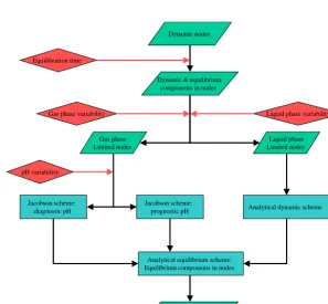
Aerosol nodes and components
Equilibration time Equilibration Mass
Dynamic solver: • 2 schemes: gas phase or pH driven
• Typically one internal time step • Some species in equilibrium
Equilibrium solver: • Nodes close to equilibrium and
numerically stiff • 2 sub-solvers: gas phase or chemically driven
Convergence Equilibrium rechecks
Equilibration mass
Updated composition Time interval
Figure 2.Formalism of HyDiS-1.0 in its hybrid configuration.
Dynamic nodes
Gas phase variability
Updated composition
Liquid phase variability Dynamic & equilibrium
components in nodes Equilibration time
Analytical dynamic scheme Jacobson scheme:
diagnostic pH pH variability
Gas phase Limited nodes
Liquid phase Limited nodes
Jacobson scheme: prognostic pH
Analytical equilibrium scheme: Equilibrium components in nodes
Figure 3.Formalism of the dynamic solver.
the model. A size class is found to be in equilibrium when its characteristic time interval corresponds to less than half the integration time step of the aerosol microphysical model the solver is embedded into, and when its equilibration re-quires less than 10 % of the total available matter for each of the dissolving species. The characteristic time interval re-flects the amount of time that would be required for the equi-libration of a size class with respect to a particular dissolv-ing species, thus neglectdissolv-ing additional equilibration time re-quirements due to chemical interaction. This definition
Equilibrium nodes
Kinetic limitation Chemical limitation
Kinetic sub-solver: •Variational principle •Mode concurrent integration •Iteration for species interaction
Chemical sub-solver: •Analytical principle •Species concurrent integration •Internal iteration for water and act. coeff.
•External iteration for node interaction
Equilibration time
Pseudo-transition correction: •Linearized adjustment for driving species •Analytical equilibration for passive species
Chemical convergence Kinetic convergence
Equilibrium composition Chemical convergence
Figure 4.Formalism of the equilibrium solver.
the equilibrium classes is calculated. In choosing to calculate equilibrium composition after the dynamic calculation fin-ished, two goals are pursued. First, equilibrium size classes tend to consume less matter than dynamic classes, as they are ideally close to equilibrium, and hence smaller. This cir-cumstance is of some relevance because their mass balance is decoupled from the dynamic size classes, thus carrying the risk of artefacts due to misrepresentation of mutual competi-tion for condensable matter. Second, it is ensured that those size classes that come close to equilibrium during integra-tion may still be put into the equilibrium mode, such that both numerical stability and computational efficiency can be ensured.
Figure 3 depicts the formalism of the dynamic sub-solver for one internal time step. First, each size class is tested for whether certain species may be assumed to be in equilibrium. This test is carried out in accordance with the above time criterion for distinction between equilibrium and dynamic classes. Species that are found to be in the dynamic regime are subdivided further according to whether their equilibra-tion is driven either by the gas phase or chemical intertion within the aqueous phase, and, in the former case, ac-cording to the variability of particle pH. As such, gas-phase-limited species are integrated in time with Jacobson’s semi-analytical method (Jacobson, 1999a), while aqueous-phase-limited species are integrated with an analytical method that provides for their larger numerical stiffness. The analytical method solves for one species in one size class, while the Jacobson method solves for one species in all size classes. The particle pH associated with the Jacobson method corre-sponds either to its momentary value (diagnostic approach), or, if found to be beyond a certain variability threshold,
to its individual species equilibrium value (prognostic ap-proach). In order to insure accurate partitioning among the size classes, time integration is performed in parallel irre-spective of the scheme that has been chosen. Finally, for the dissolving species that have been diagnosed to be in equilib-rium in some or all of the classes, the composition of the dy-namic classes is updated according to the analytical approach that is adopted in the equilibrium solver (see below).
achieved with the chemical sub-solver. Size classes that are dynamically close and chemically far from equilibrium (stiff-ness categories 3 and 4) are mostly tackled by the analytical solver. Especially classes that show numerical stiffness ac-cording to category 4 turn out to have an actual equilibration time that is far longer than the individual species’ equilibra-tion time. At each external iteraequilibra-tion of the chemical solver, the composition of these size classes is re-evaluated accord-ing to an estimation of their actual equilibration time. Size classes thus corrected are said to be in pseudo-transition and remain formally part of the equilibration process. The chem-ical sub-solver allows for a certain number of external iter-ations only. Ideally the chemical composition of the equi-librium and pseudo-transition classes converges prior to at-taining the maximum number of iterations, upon which the composition of the equilibrium classes is updated accord-ingly and the solver is exited.
4 Box-modelling evaluation 4.1 Set-up and method 4.1.1 Modelling framework
The hybrid solver was implemented in the box-model version of the modal aerosol microphysics scheme GLOMAP (Mann et al., 2010). To facilitate a clear assessment of the operation of GLOMAP–HyDiS-1.0, the box-model experiments have all microphysical processes except those specific to HyDiS-1.0 switched off. In all experiments, we assess the evolving aerosol population based on it comprising four hydrophilic modes (nucleation, Aitken, accumulation, and coarse). The particle phase in these modes is purely liquid, consisting of aqueous HSO−4, SO24−, NO−3, Cl−, NH+4, and Na+. H+ is calculated via the ion balance, taking into account the par-tial dissociation of sulfuric acid, whilst nitric acid and hy-drochloric acid are assumed to be entirely dissociated. OH− is neglected all throughout the scheme. The chemical compo-sition of sea salt is adopted from Millero et al. (2008) as Stan-dard Mean Ocean Water (SMOW), with all cations assumed to be Na+. Accordingly, the adapted composition of sea salt isaNaCl·bNa2SO4, witha=0.9508 andb=0.0492.
Gas-phase HNO3, HCl and NH3 may dissolve into and
evaporate from the aqueous phase, with activity coefficients, surface pressures and water content assessed via the Par-tial Derivative Fitted Taylor Expansion (PD-FiTE) aerosol thermodynamics scheme (Topping et al., 2009). PD-FiTE was built on the concept used in the multicomponent Tay-lor expansion method (MTEM) model of Zaveri et al. (2005) in which activity coefficients of inorganic solutes are ex-pressed as a function of water activity of the solution. Un-like MTEM, PD-FiTE was designed to remove the need for defining sulfate-poor and sulfate-rich domains. In addition, the order of polynomials that represent interactions between
binary pairs of solutes was allowed to vary to increase com-putational efficiency whilst retaining an appropriate level of accuracy. Fit to simulations from the Aerosol Diame-ter Dependent Model (ADDEM; see Topping et al., 2005a, b), the use of PD-FiTE within a dynamical framework was demonstrated for aqueous inorganic electrolytes in Topping et al. (2009) and extended for inorganic–organic mixtures in Topping et al. (2012) using the Microphysical Aerosol Nu-merical model Incorporating Chemistry (MANIC; see Lowe et al., 2009). H2SO4 is not currently considered as a
dis-solving species within HyDiS-1.0. In principle, it may be treated by the solver as a chemically interacting semi-volatile species, given that the total number of dissolving species does not exceed three, that its surface pressure would be pro-vided by the thermodynamic scheme, and that slight adap-tations to the chemical equilibrium solver are made. Alter-natively, H2SO4 could be treated by the solver as a
non-interacting semi-volatile species, or as a non-volatile species via a formal association of dissolution and condensation (Ja-cobson, 2002). Currently, H2SO4 is considered to be
non-volatile, and its condensation is simulated within a separate routine (Spracklen et al., 2005).
4.1.2 Evaluation in the equilibrium operation
One element of the box-model evaluation of GLOMAP– HyDiS-1.0 involves testing how well the equilibrium sub-solver within HyDiS-1.0 compares to the benchmark equi-librium solver AIM III (Clegg et al., 1998). In these experi-ments the gas/particle exchange of HNO3, NH3, and HCl is
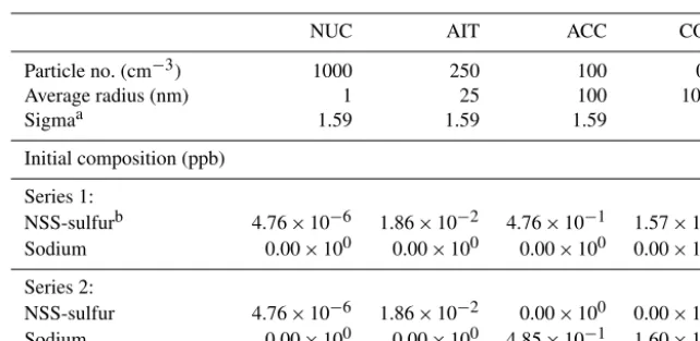
simulated with HyDiS-1.0 operating at full equilibrium. The particle composition is set up to be size-independent, consist-ing initially of a mixture of sulfuric acid, sea salt, and water. Relative humidity is set to 80 % and temperature and pres-sure to standard conditions. Three sets of these experiments are carried out with the total concentrations of NH3, HNO3,
and HCl set at equal values, being 0.1, 1, and 10 ppb. For HyDiS-1.0 these total concentrations are initially confined to the gas phase. Within each set a series of experiments is performed, as the sea salt dry volume fraction is gradually increased from 0 to 100 % (see Table 1). Surface total HNO3
and NH3mixing ratios (over the gas and particle phase) are
at most 10 ppb in polluted regions and typically around 1 ppb or less over remote oceans (Adams et al., 1999). Gas-phase HCl ranges typically from 0.001 to 0.1 ppb over the South-ern Hemisphere oceans (Erickson III et al., 1999), and is less than 10 ppb under polluted continental conditions (e.g., El-dering et al., 1991; Nemitz et al., 2004). The concentration ranges for HCl, NH3, and HNO3were not primarily chosen
Table 1.Initial particle composition (ppb) in the box-modelling evaluation against AIM III.
Volume fractiona 0 10 20 30 40 50 60 70 80 90 100
NSS-sulfurb 6.36 5.73 5.09 4.45 3.82 3.18 2.54 1.91 1.27 0.63 0.00
Sodium 0.00 0.33 0.67 1.00 1.33 1.66 2.00 2.33 2.66 2.99 3.33
aSea salt dry volume fraction (%). The densities of pure H
2SO4and sea salt are 1769 and 2196 kg m−3, respectively.bNon-sea-salt
sulfur. See text for the composition of sea salt.
Table 2.Aerosol set-up of the size-resolved box-modelling evaluations series 1 and 2.
NUC AIT ACC COA
Particle no. (cm−3) 1000 250 100 0.1
Average radius (nm) 1 25 100 1000
Sigmaa 1.59 1.59 1.59 2
Initial composition (ppb)
Series 1:
NSS-sulfurb 4.76×10⁻⁶ 1.86×10⁻² 4.76×10⁻¹ 1.57×100
Sodium 0.00×100 0.00×100 0.00×100 0.00×100
Series 2:
NSS-sulfur 4.76×10⁻⁶ 1.86×10⁻² 0.00×100 0.00×100
Sodium 0.00×100 0.00×100 4.85×10⁻¹ 1.60×100
aStandard deviation of log-normal particle size distribution. The mean volume is proportional to exp(4.5log2σ ). bSee text for sea salt composition.
de-activated this feature in the AIM III runs. The accuracy of the new solver’s equilibrium scheme can then be evaluated by comparing the surface pressures and the particle water content obtained with the two schemes. We refer the reader to Topping et al. (2009) for an assessment of the degree of accuracy that may be obtained with the simplified thermody-namic scheme PD-FiTE.
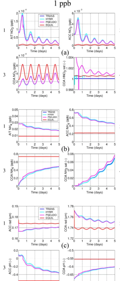
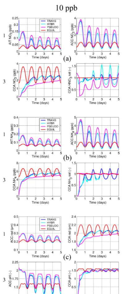
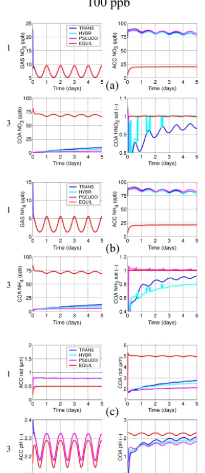
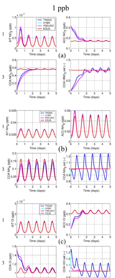
4.1.3 Evaluation in the hybrid operation
The new solver’s numerical reliability and its ability to re-produce the dynamics of the equilibration of the aerosol with the gas phase are investigated with two series of model ex-periments, one with particles within four modes initialised as binary mixtures of H2SO4and H2O, and the other with the
finest two modes initialised to contain H2SO4and H2O and
the two coarser modes (accumulation and coarse) initially containing just sea salt and H2O (see Table 2). Within
se-ries 1 only HNO3and NH3are allowed to dissolve, whereas
in series 2 HCl may dissolve additionally, thus providing for a more complex system with degassing HCl from the larger modes that can then also dissolve into the smaller modes. The fixed particle number concentrations within the log-normal modes are 1000 cm−3 (nucleation), 250 cm−3 (Aitken), 100 cm−3 (accumulation), and 0.1 cm−3 (coarse); the initial number median dry particle radii are 1, 25, 100, and 1000 nm, respectively; 5-day simulations are carried out at standard pressure and temperature conditions with
an imposed diurnal temperature cycle of±5 K starting at a maximum temperature at 18:00 LT. Relative humidity is set to 80 %. The particle number concentrations and the non-volatile species are held constant for the dissolving species to converge towards a forced dynamic equilibrium. In order to assess the model evolution across a range of numerical stiffness conditions, each of the two series involves three ex-periments with concentrations of the dissolving species set at different values. The three experiments each follow the spec-ifications above, but with the dissolving species and HNO3,
NH3, and (within series 2) HCl set to 1, 10, and 100 ppb.