Comparison of Power Flow Algorithms for inclusion in On-line Power Systems Operation Tools

(1)

University of New Orleans University of New Orleans

ScholarWorks@UNO

University of New Orleans Theses and

Dissertations Dissertations and Theses

12-17-2010

Comparison of Power Flow Algorithms for inclusion in On-line

Power Systems Operation Tools

Naveen Bokka

University of New Orleans

Follow this and additional works at: https://scholarworks.uno.edu/td

Recommended Citation Recommended Citation

Bokka, Naveen, "Comparison of Power Flow Algorithms for inclusion in On-line Power Systems Operation Tools" (2010). University of New Orleans Theses and Dissertations. 1237.

https://scholarworks.uno.edu/td/1237

This Thesis is protected by copyright and/or related rights. It has been brought to you by ScholarWorks@UNO with permission from the rights-holder(s). You are free to use this Thesis in any way that is permitted by the copyright and related rights legislation that applies to your use. For other uses you need to obtain permission from the rights-holder(s) directly, unless additional rights are indicated by a Creative Commons license in the record and/or on the work itself.

(2)

Comparison of Power Flow Algorithms for inclusion in On-line Power Systems Operation Tools

A Thesis

Submitted to the Graduate Faculty of the University of New Orleans In partial fulfillment of the Requirements for the degree of

Master of Science In

Engineering

By

Naveen Reddy Bokka

B.Tech JNTU, 2007

(3)

ii

Acknowledgement

This thesis would not have been possible without the guidance and the help of several

individuals who in one way or another contributed and extended their valuable assistance in the

preparation and completion of this study.

First and foremost, my utmost gratitude to Dr. Ittiphong Leevongwat not only for his

guidance and support in the course of my research but also for all the advice and help he

provided me throughout my graduate studies. I am also grateful to Dr. Parviz Rastgoufard for his

supervision, comments and suggestions that improved the standard of this thesis.

I am heartfelt thankful to my parents, sister and brother for all their love and support

during my studies. The same gratitude goes out to my roommates and friends who have always

supported and helped me in many ways.

Finally I would like to thank the professors and staff at the University of New Orleans for

their contribution in providing quality education. I would also like to thank UNO- Entergy Power

and Research laboratory for giving me access to special software (PowerWorld) and creating a

(4)

iii

List of Tables

Table 2.1 Bus Classification ...12

Table 4.1 Transmission Line Data ...39

Table 4.2 Transformer details ...41

Table 4.3 Generator Data ...42

Table 4.4 Loads Data ...43

Table 5.1 Test Results ...44

Table 5.2 Comparative Results of IEEE 39 system ...47

Table A.1 Comparative results of 3 bus system ...62

(7)

vi

List of Figures

Fig 2.1 3-Bus system...13

Fig 2.2 5-Bus system...15

Fig2.3 Flow Chart for load flow solution using Gauss Method ...26

Fig 2.4 Flow Chart for load flow solution using Gauss-Seidel Method ...27

Fig 2.5 Flow Chart for load flow using Newton-Raphson Method ...28

Fig 4.1 IEEE 39 bus system Model ...38

Fig 5.1 Graph using Gauss Method (Max Mismatch vs No. of iterations) ...48

Fig 5.2 Graph using Gauss Method (Max Mismatch vs Convergence time) ...48

Fig 5.3 Graph using Gauss-Seidel (Max Mismatch vs No. of iterations) ...49

Fig 5.4 Graph using Gauss-Seidel (Max Mismatch vs Convergence time) ...49

Fig 5.5 Graph using Newton-Raphson (Max Mismatch vs No. of iterations) ...50

Fig 5.6 Graph using Newton-Raphson (Max Mismatch vs Convergence time) ...50

Fig 5.7 Switching results of NR and Gauss (Max Mismatch vs No. of Iterations) ...51

Fig 5.8 Switching results of NR and Gauss (Max Mismatch vs Convergence time) ...51

Fig 5.9 Comparative results of Gauss, NR and switching technique (Iteration Number) .52 Fig 5.10 Comparative results of Gauss, NR and switching technique (Convergence time)52 Fig 5.11 Switching results of NR and GS methods (No. of iterations) ...53

Fig 5.12 Switching results of NR and GS method (Convergence time) ...53

Fig 5.13 Comparative results of GS, NR and switching technique (Iteration Number) ....54

(8)

vii

Abstract

The goal of this thesis is to develop a new, fast, adaptive load flow algorithm that “automatically

alternates” numerical methods including Newton-Raphson method, Gauss-Seidel method and

Gauss method for a load flow run to achieve less run time. Unlike the proposed method, the

traditional load flow analysis uses only one numerical method at a time. This adaptive algorithm

performs all the computation for finding the bus voltage angles and magnitudes, real and reactive

powers for the given generation and load values, while keeping track of the proximity to

convergence of a solution. This work focuses on finding the algorithm that uses multiple

numerical techniques, rather than investigating programming techniques and programming

languages. The convergence time is compared with those from using each of the numerical

techniques. The proposed method is implemented on the IEEE 39-bus system with different

contingencies and the solutions obtained are verified with PowerWorld Simulator, a commercial

software for load flow analysis.

Key Words: Power flow, Gauss method, Gauss-Seidel method, Newton-Raphson method,

(9)

1

Chapter 1 Introduction

1.1 Concept of Power Flow:

The power flow analysis is a very important tool in power system analysis. Power flow

studies are routinely used in planning, control, and operations of existing electric power systems

as well as planning for future expansion. The successful operation of power systems depends

upon knowing the effects of adding interconnections, adding new loads, connecting new

generators or connecting new transmission line before it is installed. The goal of a power flow

study is to obtain complete voltage angle and magnitude information for each bus in a power

system for specified load and generator real power and voltage conditions [1-3].

The goal of a power flow study is to obtain complete voltage angle and magnitude

information for each bus in a power system for specified load, generator real power, and voltage

conditions. Once this information is known, real and reactive power flow on each branch as well

as generator reactive power can be analytically determined. Due to the nonlinear nature of the

problem, numerical methods are employed to obtain a solution that is within an acceptable

tolerance [16].

Power flow calculation is fundamental in power systems. Power systems are non-linear

system of equations in general, the solution for these equations can be found using iterative

methods. There are several different iterative methods to solve the power flow problems. The

iterative methods give the accurate solution as they approach towards the convergence of the

(10)

2

also some direct methods that converge in less number of iterations compared to iterative

methods [3]. The memory requirements and time of calculation increases as the problem size

increases (increase in number of buses), so the direct methods are effective for small power

system problems. However, it is difficult to say which method is effective as the power flow

calculation depends on various factors like the size of the problem, the method used and the type

of problem to be solved.

In the iterative methods, the memory requirements and the number of iterations increase

as the size of the problem increases [3]. For large-sized problems only iterative methods are

proved to be efficient. In the past the problem size was small compared to the present day, hence

the direct methods were used, and there was an urgent need to find out a method that could

ensure the convergence for small-sized and large-sized problems.

The recent development in the field of digital computer technology led for the

development of a number of methods for solving the power flow problems. Some of the iterative

methods that are mainly used today are Gauss method, Gauss-Seidel method and

Newton-Raphson [5]. These methods are efficient but the comparisons between the methods are difficult

because of differences in computers, programming methods and languages, and the test

problems. However, Newton-Raphson method due to its calculation simplifications, fast

convergence and reliable results is the most widely used method of large load flow analysis.

In large-sized problems, Newton-Raphson method generates the solution in less time, but

for small-sized problems this method is not efficient in terms of time. Many research works are

still in process of finding a method that gives an efficient solution that can work for small

(11)

3

1.2 Literature review:

Power flow analysis came into existence in the early 20th century. There were many

research works done on the power flow analysis. In the beginning, the main aim of the

power-flow analysis was to find the solution irrespective of time. Over the last 20 years, efforts have

been expended in the research and development on the numerical techniques.

Before the invention of digital computers, the load flow solutions were obtained using the

network analysis. In the year 1956 the first practical automatic digital solution was found. The

early generation computers were built with less memory storage, the Y-Bus matrix iterative

method was well suitable for these computers. Although performance was satisfactory on many

power flow problems, the time taken to convergence was very slow and sometimes they never

converged [1].

In order to overcome the difficulties of this method a new method was developed based

on the Z-Bus matrix. This new method converges more reliably compared to the Y-Bus matrix

method, but it requires more memory storage when solving large problems. During this time, the

iterative methods were showing very powerful convergence properties but were difficult in terms

of computation [8]. In the mid 1960’s major changes in the power system came with the

development of very efficient sparsity programmed ordered elimination by Tinny [1].

1.3 Numerical Methods:

The concept of Power Flow problem was introduced by Carpentier in 1962. The power

system equations are non-linear in nature, Carpentier formulated a non-linear programming

(12)

4

The goal of power Flow is to minimize the total cost of meeting the load demand for the

power system while maintaining the security of the system. The developments in computer

technology helped in developing efficient algorithms for Power Flow solutions. Numerous

different mathematical techniques have been employed for solving the Power Flow problems.

Some of the existing methods used for solving Power Flow problem are Gauss method,

Gauss-Seidel method, Newton-Raphson method and Fast Decoupled Power Flow method.

The methods are briefly described in the following paragraphs:

1) Gauss method: This is an iterative method used in the calculation of power flow

analysis. This method was named after the German mathematician Carl Friedrich Gauss and

Philipp Ludwig von Seidel. It is also known as Liebmann method or the method of successive

displacement. In this method an initial value of voltage is guessed and a new value for the

voltage is calculated for each bus. In this method the new voltage value obtained at the other bus

cannot be used for the calculation of voltage at another bus until the iteration is completed. This

disadvantage is one of the disadvantages of Gauss method.

2) Gauss-Seidel method: This method is based on the Gauss method. In this method an

initial value of voltage is guessed and the newly calculated value replaces the initial value and

the iteration is stopped when the solution converges. But later this method was limited for only

small problems because of the complexity in the calculations [9].

3) Newton-Raphson method: This is the most effective iterative method used in the

present day power flow analysis. It was named after Isaac Newton and Joseph Raphson. In this

(13)

5

the result is obtained very quickly, but if the assumed value is farther away from the solution

then the method may take longer to converge [9].

4) Fast Decoupled Power Flow method: The Fast Decoupled Power Flow Method

(FDPFM) is one of the improved methods, which is based on a simplification of the

Raphson method and reported by Stott and Alsac in 1974 [7]. This method, like the

Newton-Raphson method, offers calculation simplifications, fast convergence and reliable results and

became a widely used method in load flow analysis. However, FDPFM for some cases, where

high resistance-to-reactance(R/X) ratios or heavy loading (low voltage) at some buses are

present, does not converge well. For these cases, many efforts and developments have been made

to overcome these convergence obstacles. Some of them targeted the convergence of systems

with high R/X ratios, and others with low voltage buses [28]. The FDPFM method has the

disadvantage of not yielding the accurate solution.

Though many efforts and elaborations have been achieved in order to improve the power

flow methods, these methods can still attract many researchers, especially when computers and

simulations are becoming more developed and are now able to handle and analyze large-sized

system.

Today, with processor’s speed being higher than 3 GHz, any improvement in the speed of

convergence of the power flow methods, provided it leads to reliable results, is of great value.

This speed improvement is very important when involved in operational stages of power

distribution, where any millisecond saving can hugely increase the probability of the right

(14)

6

1.4 Scope of Work:

Power flow analysis became a fundamental and important tool in the power systems these

days. Before the development of the power flow analysis on the digital computers, the power

flow was done based on network analysis. The network analysis is a time consuming method and

the convergence is not guaranteed. The backdrops of this method led for the development of

powerful computer methods. With the advancement in the fields of digital computer technologies

these power flow methods gained more importance and the solutions achieved convergence very

quickly.

The goal of this research is to develop a load flow algorithm that uses multiple numerical

methods so that the convergence time is lesser than using each traditional method alone.

Combining the benefits of different methods by switching among the methods during a single

run of load flow calculation has been proved possible in this work and resulted in the improved

run time taken to converge to a solution.

To achieve the goal, the following tasks have been performed.

1. Review the numerical techniques for load flow analysis

2. Develop the mathematical model to adaptively use multiple numerical techniques

3. Develop software program implementing the mathematical model

4. Test the algorithms with the IEEE 39-bus system

5. Develop the IEEE 39-bus system in PowerWorld as a benchmark for the load flow

solutions

6. Compare the convergence time of the switching technique with that of traditional

(15)

7

1.5 Overview:

The power flow algorithm written in this thesis is based on the Gauss-Seidel method and

Newton-Raphson method. A software program has been developed. The program gives the

power flow solution for a given problem as well as computes the complete voltage angle and

magnitude information for each bus in a power system for specified load and generator real

power and voltage conditions.

The remainder of this thesis is organized as follows. Chapter 2 of this thesis will discuss

the Gauss method, Gauss-Seidel method and Newton-Raphson method. It will also discuss the

application of each method in the power system. Chapter 3 will discuss the switching technique

used in developing the program for the power flow analysis. It will also discuss the input files

and the other terms used in developing the program in Matlab. Chapter 4 will give a detailed

explanation of the test system developed in PowerWorld. The test system developed in this thesis

is IEEE-39 bus system. The topics in this chapter include generators, loads, transmission lines,

transformers, and buses etc. used in building the IEEE-39 bus system. Chapter 5 will discuss the

test results of the proposed switching algorithm which is based on the traditional methods, tested

on the IEEE-39 bus system and compare the results with each traditional method when used by

(16)

8

Chapter 2 Application of numerical techniques to Power Flow Calculation

2.1 Numerical Techniques for Power Flow Analysis:

Power flow analysis is an evaluation process for operation and planning to determine the

steady-state condition of a power system given a condition of the system. Power flow analysis is

based on a large-scale nonlinear set of equations that require iterative techniques to obtain their

solution. There are a number of traditional iterative techniques to solve large non-linear

equations. The major methods used in the Power Systems are:

1) Gauss method

2) Gauss-Seidel method

3) Newton-Raphson method

2.1.1 Gauss method:

Gauss method is one of the oldest of the iterative techniques that is still in use in some

areas. Gauss iterative method has its own advantages and disadvantages. This technique is

simple and easy to compute. The time taken for the method to converge to a solution is generally

more compared to other iterative methods.

Consider a system of n linear equations with x unknowns:

Ax = b (2.1)

(17)

9

11 12 1

21 22 2

1 2 .. .. : : : : .. n n

n n nn

a a a

A

a a a

             , 1 2 : n x x x x             

, and

1 2 : n b b b b             

The Gauss–Seidel method is an iterative technique that solves the left hand side of this

expression (2.1) for x, using assumed value for x on the right hand side. Analytically, this may

be written as:

1

1 n

k k

i i ij j

i ii

i j

x b a x

a         _  _    



(2.2)

where k is the iteration number

The computation of xi(k+1) requires each element in x(k) except xi(k) itself. The procedure is

generally continued until the changes made by iteration are within some tolerance.

2.1.2 Gauss-Seidel method:

This is a simple iterative technique based on gauss method that was popular in the early

days of digital computer. The more powerful N-R method is however used these days.

The gauss seidel iterative technique is still used for small power systems where program

simplicity is more important than computing costs, and in many cases it is used in large scale

systems to obtain an initial solution for the continuation of Newton-Raphson method [13].

All the calculations done in gauss seidel method are same as the gauss method except in

the equation (2.2) the value of x calculated at one equation immediately replaces the x calculated

(18)

10

1 1

1

1 n

k k

i i ij j

i ii

i j

x b a x

a          _  _    



(2.3)

2.1.3 Newton-Raphson method:

The Gauss-Seidel method is very simple but convergence becomes increasingly slow as

the system size grows. The Newton-Raphson technique converges fast in less than 4-5 iterations

regardless of system size. This technique is mainly useful for large-sized system with thousands

of buses [13, 16].

Consider a function ƒ(x) = 0, and its derivative ƒ '(x), we begin with a first guess x0.

Provided the function is reasonably well-behaved a better approximation x1 is

0 1 0 0 ( ) '( ) f x x x f x

  (2.4)

Geometrically, x1 is the intersection point of the tangent line to the graph of f, with the x-axis.

The process is repeated until a sufficiently accurate value is reached:

1 ( ) '( ) k k k k f x x x f x

   (2.5)

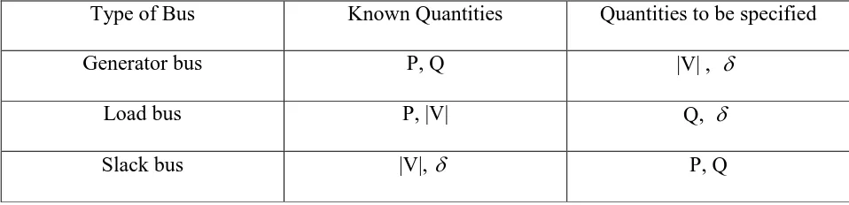
2.2 Bus Classification:

In a power system each bus or node is associated with four quantities, real and reactive

powers, bus voltage magnitude and phase angle. In a load flow solution two out of the four

quantities are specified and the remaining two are required to be obtained through the solution of

the equations. Depending upon which quantities have been specified, the buses are classified into

(19)

11

1) Generator bus or PV bus:

At this bus the voltage magnitude corresponding to the generation voltage and real power

G

P corresponding to its ratings are specified. It is required to find out the reactive power

generation Q_G and the phase angle of the bus voltage.

2) Load bus or PQ bus:

Here the real and the reactive components or power are specified. It is desired to find out

the voltage magnitude and the phase angle through the load flow solution. It is required to

specify P_D and Q_Dat such a bus at a load bus voltage can be allowed to vary within the

permissible values.

3) Slack bus or reference bus:

In a power system there are mainly two types of buses, load and generator buses. For

these buses we have specified the real power P injections. Now

1 n

i i

P





real power loss P_L

where P_i is the power injections at the buses, which is taken as positive for generator buses and

is negative for load buses. The losses remain unknown until the load flow solution is complete. It

is for this reason that generally one of the generator buses is made to take the additional real and

reactive power to supply transmission losses. That is why this type of bus is also known as the

slack bus or reference bus. At this bus, the voltage magnitude V and the phase angle  are

specified, whereas real power and reactive power P_Gand Q_G are obtained through the load flow

(20)

12

Table 2.1 Bus Classification

The phase angle of the voltage at the slack bus is usually taken as the reference. In the

following analysis the real and reactive components of voltage at a bus are taken as the

independent variables for the load flow equations i.e.

i

i i i

V   e jf

(2.6)

where e_i and f_i are the real and reactive components of voltage at the ith bus. There are various

other formulations wherein either voltage or current or both are taken as the independent

variables. The load flow equations can be formulated using either the loop or bus frame of

reference. However, from the viewpoint of computer time and memory, the nodal admittance

formulation, using the nodal voltage as the independent variables is the most economic.

2.3 Formation of Y Bus Admittance matrix:

Power system analysis, like load flow studies, short circuit studies, and transient stability

studies, has become very convenient with the advent of digital computers. More and more

complex systems can now be handled by suitable mathematical models, constituting an ordered

collection of system parameters in the form of matrices. These models depend on the selection of

independent variables. When the voltages are selected as independent variables, the

Type of Bus Known Quantities Quantities to be specified

Generator bus P, Q |V| , 

Load bus P, |V| Q, 

(21)

13

corresponding currents are dependent and the matrix relating the voltages to the currents is then

in the admittance form. When these voltages and currents are referred to the buses (independent

nodes), the reference is the bus frame, and the resulting equations are usual independent nodal

equations. The voltages and currents, when referred to independent loops, are related by the

admittance matrix in the loop frame of reference. When the currents are treated as independent

variables, the matrices are impedance matrices in the respective frames of reference.

It is seen from the study of the literature that these bus admittance and impedance

matrices, as well as loop admittance and impedances, have been widely used for various power

system calculations. There are traditional methods of forming these matrices for a given system,

which require various connection or incidence matrices. Algorithms for forming the bus

impedance matrix and its dual, the loop admittance matrix, have been developed and are widely

used in various system studies [14]. Fig 2.1 clearly explains the formation of Nodal Admittance

matrix. The load flow equations, using nodal admittance formulation for a three-bus system are

developed first and then they are generalized for an n-bus system.

(22)

14

At node 1:

I1 I11I12I13

= V y_{1 11}(V₁V y₂) ₁₂(V₁V y₃) ₁₃

= V y₁( ₁₁y₁₂y₁₃)V y_{2 12}V y_{3 13}

1 1 11 2 12 3 13

I V Y V Y V Y (2.7)

11

Y is the diagonal element and Y₁₂, Y₁₃ are the off diagonal elements, and these can be calculated

using 1, 1 n ij

i i j ij ij

Y

r jx

 







for off diagonal elements (2.8)

1,

n

ii ij

i i j

Y Y

 





for on diagonal elements (2.9)

where in this case y11 is the shunt charging admittance at bus 1 and

11 11 12 13

Y  y y y

12 12

Y  y

13 13

Y  y

Similarly nodal current equations for the other nodes can be written as follows

2 1 21 2 22 3 23

I V Y V Y V Y (2.10)

3 1 31 2 32 3 33

I V Y V Y V Y (2.11)

These equations can be written in a matrix form as:

1 11 12 13 1

2 21 22 23 2

3 31 32 33 3

I Y Y Y V

     

  _   

     

(23)

15

or in a compact form equation (2.12) can be written as:

3

1

i ij j j

I Y V





, p = 1 to 3 (2.13)

From this we now write nodal current equation for n bus system where each node is connected

to all other nodes.

1

n

i ij j j

I Y V





, p = 1, 2… n (2.14)

Equation 2.14 can be represented in matrix form as

1 11 12 1 1

2 21 22 2 2

1 2 .... .... : : : .... : : .... n n

n n n nn n

I Y Y Y V

              _                      (2.15)

It can be observed that the nodal admittance matrix is a sparse matrix (a few number of elements

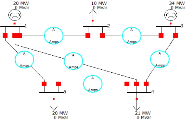
are non-zero) for an actual power system. Consider Fig.2.2

(24)

16

The nodal admittance matrix for system in Fig 2.2 is as follows:

11 12 14 15

21 22 23

32 33 34

41 43 44 45

51 54 55

0 0 0 0 0 0 0 0 bus

Y Y Y Y

Y Y Y

Y Y Y Y

Y Y Y

                 (2.16)

It can be observed that out of 25 elements, eight elements are zero whereas 17 are

non-zero. In a large system of 100 nodes, these non-zero elements may be as small as 2% of the total

elements. This is where we see that the computer memory requirement for storing the nodal

admittance matrix is very low. It need store only a very few non-zero elements, it need not stare

the zeros of the matrix. Again the nodal admittance being a symmetric matrix along the leading

diagonal, the computer need store the upper triangular nodal admittance matrix only. Thus, the

computer memory requirement for storing the nodal admittance is all the more reduced.

If the interconnection between the various nodes for a given system and the admittance

value for each interconnecting circuit are known, the admittance matrix may be assembled as

follows:

a) The diagonal element of each node is the sum of the admittances connected to it.

b) The off-diagonal element is the negative admittance between the nodes.

However, it can be seen that the sum of the elements in each columns of the admittance

matrix summates to zero which means that nodal admittance matrix is a singular matrix and

hence the rows of the matrix are linearly dependent.

We have already justified the necessity of selecting one of the buses as the slack or reference bus

based on power balance in the system. Based on the admittance matrix approach, it can be said

(25)

17

singular and cannot be handled. By taking one of the buses as reference, corresponding row and

column are deleted from the nodal admittance matrix and hence the reduced matrix becomes

non-singular, which can be handled very easily.

2.4 Formation of Power Flow Equations:

The power flow problem is the computation of voltage magnitude and phase angle at

each bus in a power system under system steady conditions. As a by-product of this calculation,

real and reactive power are calculated, as well as equipment losses, can be computed [30]. The

input data for the power flow consists of bus data, transmission line data, and transformer data .

The first step in a power flow is the calculation of bus admittance matrix Y bus, the Y

bus can be constructed from the transmission line and transformer input data (Formulation of Y

bus admittance matrix is explained in section 2.3).

Using Y bus, we can write nodal equation for a power system network as:

bus

I  Y V

(2.17)

where I is the n column vector of source currents injected into each bus and V is the n

column vector of bus voltages. For bus k, the kth equation in (2.17) is:

1

n

i ij j j

I Y V





(2.18)

The complex power delivered to bus k is

*

i i i i i

S  P jQ V I

(2.19)

Power flow equations by Gauss and Gauss-Seidel are based on nodal equations (2.18), where

(26)

18

*

1

n

i i i i ij j

j

S P jQ V Y V



 

  _{ } _





 (2.20)

i = 1, 2, 3………n

(2.20) can be rewritten in polar form as

( )

1

i j ij n

j i i k ij j

j

P jQ V Y V e    



 



(2.21)

Taking the real and imaginary parts of (2.21), power balance equations can be written as

1

cos( )

n

i i ij j i j ij j

P V Y V   





  (2.22)

1

sin( )

n

i i ij j i j ij j

Q V Y V   





  (2.23)

or when the Y_ki is expressed in rectangular coordinates

1

[ cos( ) sin( )]

n

i i j ij i j ij i j

j

P V V G   B  





   (2.24)

1

[ sin( ) cos( )]

n

i i j ij i j ij i j

j

Q V V G   B  





   (2.25)

where Gij |Yij| cos(ij) (2.26)

| | sin( ) ij ij ij

B Y  (2.27)

2.5 Algorithms for Power Flow methods:

Gauss-Seidel method is an iterative method for solving a set of non-linear equations. This

method starts with an assumption of a set of solution vector. In this method the new calculated

(27)

19

subsequent equations. This process is repeated for all the other variables for the completion of

current iteration. If the solution is converged to a certain tolerance value then the iteration is

stopped else the iteration process is repeated till convergence is achieved. This method is more

dependent on the initially assumed values.

The general load flow equation of the Gauss method is:

*

* 1

1 n

i

i ij j

j ii i

j i S

V Y V

Y V        _  _    



(2.28)

where v is the iteration number

Equation (2.28) can be rewritten in a new form to update the value of V_ik with new calculated

voltage V_ik1 :

1 _* 1 1 ( ) i k _n i k k

i k ij j

j ii i

j i P jQ

V Y V

Y V     _     _  _    



(2.29)

In Equation (2.29) the value of the reactive power Q_ifor a generator bus is unknown and

can be calculated from the equation (2.25). As a general start the initial voltage magnitude |Vi|

and the phase angle _i can be initialized to 1pu and 0 degrees. In doing so, there are total of

(n-1) load flow equations for n buses as the voltage magnitude and the phase angle for the slack bus

are already specified and the remaining unknown’s real power P_i and the reactive power Q_i can

be calculated from the power flow equations (2.24) and equation (2.25).

The value of the reactive power calculated at the generator bus has to be checked if this

(28)

20

power generation or more than the maximum reactive power generation).If it violates the

reactive power generation limits than the bus time will be switched to load bus for that iteration.

If Q_i is less than Q_min then it will be set to Q_min or if Q_i is more than Q_maxthen it will be set to

max

Q . If the reactive power is within the limits, it is substituted in the equation for the calculation

of the voltage magnitude.

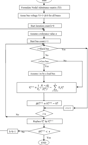
2.5.1 Algorithm for Gauss method:

Gauss Method is done by the following steps:

Step 1: Form the nodal admittance matrix (Y_ij).

Step 2: Choose a tolerance value .

Step 3: Assume the initial voltage values to be 1pu and 0degree except for the slack bus.

Step 4: Start iteration for bus i =1 with count 0.

Step 5: Check for the slack bus if for i=slack bus or PV bus update the value of Q_i using

equation (2.25).

Step 6: Calculate the new bus voltage V_i from the load flow equation (2.27).

Step 7: Find the difference in the voltages



V

_ik1



V

_ik1



V

_ik

Step 8: Go for the next bus and repeat the steps 5 to 7 until a new set of values V_ik1 of

bus voltages are obtained for all the buses.

Step 9: Continue the iteration from 5 to 9 until the value of V_ik at all the buses is within

(29)

21

V_ik1

where k gives the number of iterations.

The algorithm for gauss method is depicted in Figure 2.3.

2.5.2 Algorithm for Gauss-Seidel (GS) Method:

Gauss-Seidel Method is done by the following steps:

Step 2: Choose a tolerance value .

Step 3: Assume the initial voltage values to be 1pu and 0degree except for the slack bus.

Step 4: Start iteration for bus i =1 with count 0.

Step 5: Check for the slack bus if for i=slack bus or PV bus update the value of Q_i using

equation (2.25).

Step 6: Calculate the new bus voltage V_i from the load flow equation (2.27).

Step 7: Find the difference in the voltages



V

_ik1



V

_ik1



V

_ik

Step 8: The new calculated value of the bus voltage is updated in the old bus voltage

value and is used for the calculations at the next bus.

Step 9: Go for the next bus and repeat the steps 5 to 7 until a new set of values of bus

voltages are obtained for all the buses.

Step 10: Continue the iteration from 5 to 9 until the value of V_ik at all the buses is

within the chosen tolerance value

(30)

22

where k gives the number of iterations.

The algorithm for Gauss-Seidel method is presented as a diagram in Figure 2.4.

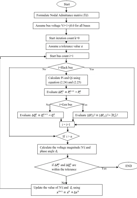
2.5.3 Algorithm for Newton-Raphson (NR) method:

Power flow solutions by Newton-Raphson are based on the nonlinear power-flow

equations given by (2.24) and (2.25).

Equations (2.24) and (2.25) are analogous to the nonlinear equation of the form y = f(x),

we define x, y and f are vectors for the power flow problem as

Let the composite vector of  and |V| is

| | x V         2 3 : : n                      and 2 3 | | | | | | : : | | V V V Vn                  and 2 2 : : n n P P P y Q Q Q           _{ }_{  }             (2.30) ( ) ( ) ( ) P x

f x y

Q x

 

   

  (2.31)

where all V, P and Q terms are in per-unit and  terms are in radians. The slack bus

(31)

23

Newton-Raphson method is a complex calculation involving derivative of real power and

reactive power with respect to V and . Jacobian matrix is the matrix formed out of the

derivatives of power with V and  and is indicated by J, where

11 12 21 22 J J J J J     

  (2.32)

Where ₁₁ i( )

j P x J     12 ( ) | | i j P x J V   

₂₁ i( )

j Q x J     22 ( ) | | i j Q x J V  

 i = 1, 2, 3… n and j = 1, 2, 3… n

The iterative process for Newton-Raphson method:

( )

k k k

J   x f x (2.33)

2 2( )

( ) :

( )

n n

P P x

P x

P P x

      _{ } _      (2.34)

2 2( )

( ) :

( )

n n

Q Q x

Q x

Q Q x

      _{ } _      (2.35) ( ) P x

(32)

24 ( ) ( ) ( ) P x f x Q x      _ 

  (2.36)

It is well known that a small change in phase angle changes the flow of active power and

does not affect much the flow of reactive power. Similarly a small change in nodal voltage

affects the flow of reactive power whereas active power practically does not change. Keeping

these facts in mind and using the polar coordinates, the set of linear load flow equations can be

written in matrix form as follows:

11 12

21 22

( )

| | ( )

k k k k

J J P x

J J V Q x



      



  _  _ 

   

  (2.37)

Here J₁₁ correspond to the elements i( )

j

P x 



 which exist and are not zero in most cases.

J₁₂andJ₂₁corresponds to the elements ( )

| | i j P x V 

 and

( ) i j Q x  

 respectively which does not exist

and, therefore, are zero.

J₂₂ corresponds to the elements ( )

| | i j Q x V 

 which exist and are not zero.

To findxk1, equation (2.37) is solved for xk and use equation (2.38). At this point the

mismatch vector and the Jacobian matrix are updated and the iteration is continued.

1

k k k

(33)

25

Steps to perform Newton-Raphson method:

Step 2: Assume an initial set of bus voltage and set bus n as the reference bus.

Step 3: Calculate the real Power P_i using the equation (2.24).

Step 4: Calculate the reactive Power Q_i using the equation (2.25).

Step 5: Form the Jacobian matrix.

Step 6: Find the power differences P_i and Q_i for all the i=1, 2, 3… (n-1).

Step 7: Choose the tolerance values.

Step 8: Stop the iteration if all P_i and Q_i are within the tolerance values.

Step 9: Substitute the values obtained in step 4 and step 5 in the equation (2.30), and then

find the vectors  and | |

| |

i

V V



Step 10: Update the values |V_i| and _ifor all i , using xk1 xk  xk

Step 11: Repeat the steps from 3.

(34)

26

Yes

No

Yes

No

Yes

Formulate Nodal Admittance matrix (Yij) Start

Assue bus voltage Vi=1+j0.0 for all buses

Start iteration count k=0

Assume a tolerance value

Start bus count i=1

i=Slack bus

i=Gen bus

Assume i to be a load bus

∑

i<n

Replace

END k=k+1

i=i+1

(35)

27 Yes No No Yes No No No Yes

Formulate Nodal Admittance matrix (Yij) Start

Assume bus voltage Vi=1+j0.0 for all buses

Start bus count i=1 i=Slack bus

i=Gen bus

Calculate Real and Reactive power using eq (2.24)&(2.25)

Assume i to be a load bus

∑ ∑ Replace i=i+1 i<n k=k+1 END

(36)

28

No Yes

Yes

No

Formulate Nodal Admittance matrix (Yij)

Start

Assume bus voltage Vi=1+j0.0 for all buses

Start bus count i=1 i=Slack bus

Calculate Pi and Qi using equation (2.24) and (2.25)

Evaluate

i=Gen bus

i = i+1

If i > n

Calculate the voltage magnitude |Vi| and phase angle

if and are within the tolerance

END

Update the value of |Vi| and using

(37)

29

2.6 Concept of Big O Notation:

Big O notation is used to describe the performance or complexity of an algorithm. Big O

specifically describes the worst-case scenario, and can be used to describe the execution time

required or the space used (e.g. in memory or on disk) by an algorithm [9]. Big O notation

characterizes functions according to their growth rates: different functions with the same growth

rate may be represented using the same O notation.

Although developed as a part of pure mathematics, this notation is now frequently also

used in the analysis of algorithms to describe an algorithm's usage of computational resources:

the worst case or average case running time or memory usage of an algorithm is often expressed

as a function of the length of its input using big O notation. This allows predicting the behavior

of their algorithms and to determine which of multiple algorithms to use, in a way that is

independent of computer architecture or clock rate. Because Big O notation discards

multiplicative constants on the running time, and ignores efficiency for low input sizes, it does

not always reveal the fastest algorithm in practice or for practically-sized data sets, but the

approach is still very effective for comparing the scalability of various algorithms as input sizes

become large [9].

The worst case scenario will give the maximum run time. Any improvement in the worst

case to make it an average case or best case will result in improved run time. As a part of

literature review Big O notation was used to study the order and the behavior of the traditional

methods. The order of Gauss method and Gauss-Seidel method is same as they have the same

algorithm except the Gauss method do not replace the calculated values in the same iteration and

(38)

30

is high compared to Gauss methods, as it involves the calculation of Jacobian matrix which is an

n by n matrix of all first-order partial derivatives of a vector- or scalar-valued function with

respect to another vector. From the order of the method it is clear that the average run time and

algorithm complexity of Newton-Raphson method is high. This makes the Gauss methods

advantageous over Newton-Raphson method for small system which converges in less number of

iterations. Hence, it can be observed that the method to be used to run a power flow solution also

(39)

31

Chapter 3 Power Flow Calculation

This chapter discusses the development of the new algorithm, development of the

program to implement the used algorithm.

3.1 Switching technique:

While performing the power flow it is often necessary to obtain an accurate result with

less convergence time. For a small system as can be observed from the results for 3-bus and

5-bus systems the convergence time is not very high, in this case any of the traditional method can

be used to find the power flow. For a large-size system where the convergence time is high the

selection of best method plays a vital role.

The switching technique is performed using two traditional methods to perform the load

flow problem. The first step is to produce a good initial condition for the second method and the

second step is to generate an accurate solution.

The switching method can be done in any of the following order

1) Start with Newton-Raphson method and then switch to gauss method

2) Start with Newton-Raphson method and then switch to gauss-seidel method

3) Start with gauss method and then switch to Newton-Raphson method

(40)

32

Selection of the switching order differs from one system to another depending on the size

of the system. It is expected that switching between two methods yields a faster convergence

time compared to running a power flow on one traditional method.

The first method starts with an assumed initial values and a least tolerance value. When

the solution is within the tolerance value the load flow is stopped for the first method and

switched to second method. The results thus obtained from the first method are taken as the

initial values for the second method. The second method starts with these initial values and a

good tolerance values. The load flow is run until the solution converges with the second

method.

Small System:

For a small system the selection of traditional methods can be in the order of Gauss

method, Gauss-Seidel method and Newton-Raphson method. The selection is mainly based on

the average convergence time and total convergence time. It is expected that the number of

iterations for this system is less and so is the total convergence time. In this case the method

with less average convergence time is expected to give better convergence time than high

average iteration time method. The average iteration time of Gauss and Gauss-Seidel method is

less compared to the Newton-Raphson method. Moreover the total convergence time using

Gauss and Gauss-Seidel method is almost less than or equal to the time taken to complete one

iteration of Newton-Raphson method. In this case switching from one method to another does

not yield any advantage over the traditional method. The 3-bus and 5-bus test systems are used

(41)

33

Large System:

For a large system the selection of traditional methods can be in the order of

Newton-Raphson method, Gauss-Seidel method and Gauss method. The selection is mainly based on the

average convergence time and total convergence time. It is expected that the number of iteration

for this system are large and so is the total convergence time. In this case the method with less

number of iteration gives better convergence time than large number of iterations.

For a large system the first method is either Gauss method or Gauss-Seidel method and the last

method will be Newton-Raphson method. As Newton-Raphson converges faster than Gauss and

Gauss-Seidel method it is desired to follow this order. Taking into account the total number of

iterations, the system achieves convergence in relatively less number of iterations. Typically the

first method should run 0.1 tolerance value and then switched to another method till an accurate

solution is achieved with 0.001 tolerance value. IEEE 39-bus test system is used to test the

switching order.

3.2 Development of software to implement the new switching algorithm:

Power flow solution yields valuable information regarding a power system, the

implementation of the numerical techniques in a power system simulation environment holds

even greater promise. In this environment, simulation of a system over time can be done while

maintaining it at its optimal condition. In this section all the programming technique, with the

(42)

34

3.2.1 Input Files:

The input files for this program to execute are the transmission line data, transformer

details, generators, loads.

The transmission line data will have matrix five columns. The first two columns (from

bus & to bus) will give the details of the buses which are connected with the transmission lines.

Third column is for the resistance of the respective transmission line connected to the buses in

column 1 and 2. Fourth column has the reactance of the transmission line and the fifth column

has the susceptance of the transmission line. All the parameters of the transmission line are taken

in p.u. The transformer details are similar as transmission line except the transformer input

matrix will have only four columns, it does not have the susceptance column.

The generator input is a matrix with five columns and as many number of rows as the

generators. The first column will have the details of the bus number to which the generator is

connected. The second column is to specify the generator number, this column is of no

importance while the time of execution but is used to generate a detailed output format. The third

column specifies the rated voltage of the generator in kv. The fourth column gives the p.u

voltage value of the generator. The fifth column is to specify the active power of the generator

before the execution. The load input is almost similar to the generator matrix with additional

reactive power details.

3.2.2 Initial Condition:

All the iterative methods are more or less sensitive to initial assumed values. For a load

(43)

35

properties and its behavior to the initial values. The closer the initial assumed value to the

solution the faster is the convergence achieved and vice versa. In this load flow programs the

initial values are the magnitude of the voltage at the bus and the angle at bus.

The voltage magnitude at the generator buses are specified in the input generator matrix,

they are to be maintained fixed throughout the load flow run while finding the optimal solution.

For buses other than the generator buses the unknown values the voltage magnitude and the

angle are assumed before running the load flow solution.

Typically, the voltage magnitude and angle are specified 1.0 p.u and 0 degree

respectively. Once the initial values are assumed then the load flow is run to obtain an optimal

solution. During the load flow run these initial values are replace with the values that are close to

the solution and as the final result an optimal values of the voltage magnitude and angle

is obtained.

3.2.3 Tolerance:

Tolerance value is an important factor that determines the accuracy of the solution.

Typically, most of the programmers take 0.001 as the tolerance value. If tolerance value is

chosen less than 0.001 the solution converges in less time and less iteration. For a higher

tolerance value convergence time and iteration number is high. But, as the tolerance value

increases the accuracy of the solution increases. At certain value of tolerance the solution attains

(44)

36

Total Convergence time:

Convergence time is a measure of how fast a power flow reaches the state of

convergence. Total convergence time is the total time elapsed after the system is converged. It is

one of the main goals of an algorithm to implement a mechanism that allows all the conditions

and inputs to quickly and reliably converge. Of course, the size of the network also plays an

important role; a larger network will converge slower than a small one.

Certain loads and generator conditions will prevent a power flow from ever converging

and lead to a blackout situation. For instance, if the total load of the system is much higher than

the maximum generating capacity of all generators, this might cause a system blackout and never

converge for the current. Under certain circumstances it might even be desired to change the

inputs or the assumed initial conditions to force the system to converge.

Average convergence time:

In numerical analysis, the speed at which a convergent sequence approaches its limit is

called the rate of convergence or average convergence time. Although strictly speaking, a limit

does not give information about any finite first part of the sequence, this concept is of practical

importance if we deal with a sequence of successive approximations for an iterative method, as

then typically fewer iterations are needed to yield a useful approximation if the rate of

convergence is higher. This may even make the difference between needing ten or a million

iterations [29].

Average convergence time or average iteration time is the time elapsed for an iteration to

complete. It can be calculated by taking the average of total convergence time by the total

(45)

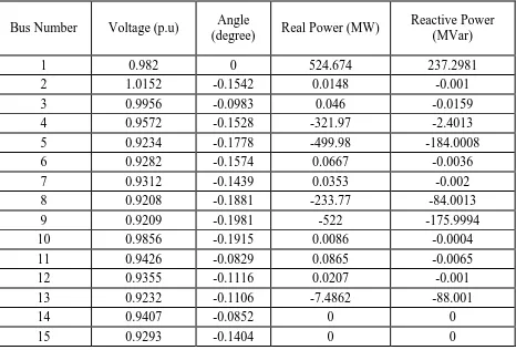
37

Chapter 4 IEEE 39 bus Test System

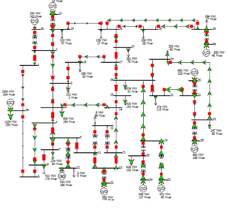
4.1 IEEE-39 bus system details:

The IEEE-39 bus system is built in PowerWorld and is used to find the power flow using

the following methods

1) Gauss method

2) Gauss-Seidel method

3) Newton-Raphson method

and the time taken to get the solution in these methods is calculated.

The details of the IEEE-39 bus system are [15]:

Number of buses – 39

Number of generators – 10

Number of loads – 19

Number of transmission lines – 34

Number of transformers – 12

The buses with generators connected to it are called the generators buses or PV buses.

The buses with loads connected to it are called the load buses or PQ buses.

(46)

38

(47)

39

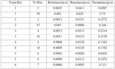
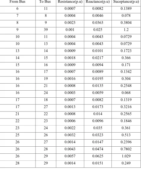
4.2 Transmission Lines:

As stated in section 4.1 the IEEE-39 bus system has 34 transmission lines. The

transmission lines are used to connect the various buses. Each transmission line is of different

length depending on how far the two buses are located, and each transmission line has its own

resistance, impedance and suceptance. But for this particular thesis work the length of the

transmission line is not of much concern.

The details of all the transmission lines with its resistance, impedance and suceptance and

the connection from which bus to other bus are listed in the table 4.1.

Transmission Line data:

From Bus To Bus Resistance(p.u) Reactance(p.u) Suceptance(p.u)

1 2 0.0035 0.0411 0.6987

1 39 0.001 0.025 0.75

2 3 0.0013 0.0151 0.2572

2 25 0.007 0.0086 0.146

3 4 0.0013 0.0213 0.2214

3 18 0.0011 0.0133 0.2138

4 5 0.0008 0.0128 0.1342

4 14 0.0008 0.0129 0.1382

5 6 0.0002 0.0026 0.0434

5 8 0.0008 0.0112 0.1476

6 7 0.0006 0.0092 0.113

(48)

40

From Bus To Bus Resistance(p.u) Reactance(p.u) Suceptance(p.u)

6 11 0.0007 0.0082 0.1389

7 8 0.0004 0.0046 0.078

8 9 0.0023 0.0363 0.3804

9 39 0.001 0.025 1.2

10 11 0.0004 0.0043 0.0729

10 13 0.0004 0.0043 0.0729

13 14 0.0009 0.0101 0.1723

14 15 0.0018 0.0217 0.366

15 16 0.0009 0.0094 0.171

16 17 0.0007 0.0089 0.1342

16 19 0.0016 0.0195 0.304

16 21 0.0008 0.0135 0.2548

16 24 0.0003 0.0059 0.068

17 18 0.0007 0.0082 0.1319

17 27 0.0013 0.0173 0.3216

21 22 0.0008 0.014 0.2565

22 23 0.0006 0.0096 0.1846

23 24 0.0022 0.035 0.361

25 26 0.0032 0.0323 0.513

26 27 0.0014 0.0147 0.2396

26 28 0.0043 0.0474 0.7802

26 29 0.0057 0.0625 1.029

28 29 0.0014 0.0151 0.249

(49)

41

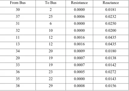
4.3 Transformers:

The model is built with 12 transformers connected at various buses. Those details consist

of RT (Resistance) and XT(Reactance) which are equivalent resistance and reactance referred

with respect to primary or secondary. For this system assume those values are with respect to

primary winding of the transformer.

All the values in above table are in per unit. For this system transformer at generators

primary winding is delta lag with rated voltage of 20KV. Secondary winding is star grounded

with rated voltage of 345KV. All the remaining transformers are grounded stat-star with both the

windings rated at 345KV. Transformer details are given in the table 4.2.

Transformer details:

From Bus To Bus Resistance Reactance

30 2 0.0000 0.0181

37 25 0.0006 0.0232

31 6 0.0000 0.0250

32 10 0.0000 0.0200

11 12 0.0016 0.0435

13 12 0.0016 0.0435

34 20 0.0009 0.0180

20 19 0.0007 0.0138

33 19 0.0007 0.0142

36 23 0.0005 0.0272

35 22 0.0000 0.0143

38 29 0.0008 0.0156

(50)

42

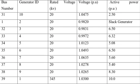
4.4 Generator Buses:

The IEEE-39 bus system has total of 10 generators. The buses for which generators are

connected to it are called the generator buses or PV-buses. For all the generator buses the value

of the real power P (MW) and the magnitude of the voltage are known and the unknown values

are the reactive power Q (MVAr) and angle of the voltage. The generator buses in this case are

from the bus 30 to 39.

The detail information of all the generators with their respective bus numbers are listed in

the table 4.3.

Generators Details:

Table 4.3 Generators Bus

Number

Generator ID Rated Voltage

(kv)

Voltage (p.u)

Active power

(p.u )

31 10 20 1.0475 2.50

1 2 20 0.9820 Slack Generator

32 3 20 0.9831 6.50

33 4 20 0.9972 6.32

34 5 20 1.0123 5.08

35 6 20 1.0493 6.50

36 7 20 1.0635 5.60

37 8 20 1.0278 5.40

38 9 20 1.0265 8.30

Comparison of Power Flow Algorithms for inclusion in On-line Power Systems Operation Tools

ScholarWorks@UNO

ScholarWorks@UNO

Comparison of Power Flow Algorithms for inclusion in On-line

Comparison of Power Flow Algorithms for inclusion in On-line

Power Systems Operation Tools

Power Systems Operation Tools

Acknowledgement

Contents

List of Tables

List of Figures

Abstract

Chapter 1

Introduction

1.1 Concept of Power Flow:

1.2 Literature review:

1.3 Numerical Methods:

1.4 Scope of Work:

1.5 Overview:

Chapter 2

Application of numerical techniques to Power Flow Calculation

2.1 Numerical Techniques for Power Flow Analysis:

2.1.1 Gauss method:



2.1.2 Gauss-Seidel method:



2.1.3 Newton-Raphson method:

2.2 Bus Classification:



2.3 Formation of Y Bus Admittance matrix:









2.4 Formation of Power Flow Equations:















2.5 Algorithms for Power Flow methods:





2.5.1 Algorithm for Gauss method:



V



V



V

2.5.2 Algorithm for Gauss-Seidel (GS) Method:



V



V



V

2.5.3 Algorithm for Newton-Raphson (NR) method:

2.6 Concept of Big O Notation:

Chapter 3

Power Flow Calculation

3.1 Switching technique:

3.2 Development of software to implement the new switching algorithm:

3.2.1 Input Files:

3.2.2 Initial Condition:

3.2.3 Tolerance:

Chapter 4

IEEE 39 bus Test System

4.1 IEEE-39 bus system details:

4.2 Transmission Lines:

4.3 Transformers:

4.4 Generator Buses: