Online Detection of Hydrodynamic Changes in Fluidized Bed using Cross Average Diagonal Line

(1)

53 H. Ziaei-Halimejani et al. / Journal of Chemical and Petroleum Engineering, 50 (2), Feb. 2017 / 53-60

Online Detection of Hydrodynamic Changes

in Fluidized Bed using Cross Average

Diagonal Line

Hooman Ziaei-Halimejani,

**Reza Zarghami* and Navid Mostoufi**

Multiphase Systems Research Lab, School of Chemical Engineering, College of Engineering, University of Tehran, P.O. Box 11155/4563, Tehran, Iran.

(Received 10 April 2016, Accepted 26 June 2016)

Abstract

Online detection of hydrodynamics of gas-solid fluidized bed was char

-acterized using pressure fluctuations by cross recurrence plot (CRP) and cross recurrence quantification analysis (CRQA). Experiments were conducted in a lab scale fluidized bed of various particle sizes 150 µm, 280 µm and 490 µm at different gas velocities. Firstly, pattern changes of cross recurrence plot were discussed and then reference

states was selected. Afterwards, cross average diagonal line (CLave) of

other states corresponding to reference states were obtained. It was found that cross average diagonal line of non-normalized data initially decreases and then increases with increasing the gas velocity. When the signal is initially normalized, cross average diagonal line does not change with the superficial gas velocity. It was concluded that cross

average diagonal line could be used for detecting small changes of par

-ticle size and if a proper reference state is chosen, it can be perceived as a powerful index for detecting changes in the size of particles in a fluidized bed.

Keywords

Cross recurrence quantifica

-tion analysis;

Fluidized bed;

Cross average diagonal line; Pressure fluctuations;

Online detection.

Introduction

1 * Corresponding Author.

E-mail: [email protected] (R. Zarghami)

1. Introduction

G

as-solids fluidized beds are extensively used

in the industries owing various multiphase

flow such as petroleum, petrochemical, chem

-ical, mineral, biochem-ical, pharmaceut-ical, food, etc. The wide application of fluidized beds is due to

their high efficiency of mass and heat transfer, ther

-mal homogeneity, high mixing ability and effective contact between solid and fluid [1]. Fluidized bed

reactors are among the most complex unit opera

-tions due to nonlinear dynamics of the two-phase flow. As a result, modeling the hydrodynamics of these reactors are a challenge due to the complexity

of their governing equations [2]. Pressure fluctua

-tion of the gas inside the bed is an essay to measure

variable process that includes information about many different dynamic phenomena occurring in

the bed. These include gas turbulence, bubbles

hy-drodynamics and the effect of bed operating condi

-tions [3, 4].

Several methods can be used for analyzing the

time-series in the state space [5-10]. In these anal

(2)

threshold is specified and the plot is defined as:

(1)

where N is the number of measured points, , ε

is threshold distance, Θ(.) is the Heaviside function

and |.| is a norm for indicating the difference

be-tween trajectories. The Heaviside function is a tool for comparing two trajectories. If difference of each trajectories is greater than ε the Heaviside function will be equal to zero, R_i,j(ε)=0. In opposite, if the distance is less than ε, the Heaviside function will

be equal to one, R_i,j(ε)=1. For plotting this matrix, a black dot is shown where R_i,j(ε)=0 and a white

dot where R_i,j(ε)=1. According to its definition, RP

is a symmetric plot and its main diagonal is black. According to this definition, each point shows the

recurrences of dynamical system states.

2.2 Cross Recurrence Plot

CRP is an extension of RP which is capable of ana

-lyzing dependencies of two dynamical systems in all times by comparing their states [20]. The CRP investigates the dynamics of two systems in one phase space and then displays it into a plot. The cross recurrence matrix is defined as:

(2)

where N is the number of first measured variable

and M is the number of second measured vari

-able . In the CRP, the length of measured vari-ables,

and , are not to be necessarily equal. However,

in the present work, N and M were considered to

be equal and the trajectories on phase space were

constructed based on the time-series for both

sys-tems. Due to the difference in the two systems, the main diagonal of CRP is not entirely black and the plot is not symmetric. Moreover, according to this

definition a black dot in the CRP is not an indica

-tion of the recurrence of system but declares the

similarity states between the two systems.

2.3 Cross Recurrence Quantification Analysis

Quantification of CRP structures is performed by applying the CRQA. The CRQA determines how and how often the two systems show similar patterns

of change or movement. CRQA parameters are de

-fined such that they would have a physical inter

-pretation. Some of these parameters are defined

based on the diagonal structures and are used for

articulating the coordination of two systems. One [11] with the help of statistical methods such

as S-statistic [12] and Z-statistic [13]. The main drawbacks of these methods are long-term data

requirement, time-consuming calculations and

un-certainty in determination of embedding parame

-ters [14]. Recently, several researchers have utilized the recurrence plot (RP) to analyze the nonlinear time-series. The concept of the RP and recurrence quantification analysis (RQA) was introduced by Eckmann et al. [2, 15] and developed to describe

the behavior of the system in the phase space. Hy

-drodynamics of fluidized bed was also investigated by RP and RQA and it was shown that the RP is a

powerful and easy method for monitoring and de

-tecting changes of the flow patterns in a fluidized bed [16]. The online monitoring of hydrodynamic status of a fluidized bed was explored using RP and

its capability to predict sudden changes was com

-pared with the S-statistic method which revealed its high sensitivity [17]. Also, Sedighikamal et al. [18] used one of CRQA parameters to show ability of this method to investigate the velocity transition.

Tahmasebpoor et al. [19] investigated the hydro

-dynamics of fluidized beds by RP and showed its advantage in comparison to statistical and wavelet

transform techniques.

In this work, monitoring method based on the cross recurrence plot (CRP) proposed by Marwan et al. [20], as a bivariate extension of RP, is applied

to online detection of hydrodynamics of bubbling

fluidized beds through measurement of bed pres

-sure fluctuations. Effect of superficial gas velocity and particle size on the hydrodynamics of the bed is investigated with cross average diagonal line

(CLave).

2. Theory

2.1 Recurrence Plot

Recurrence plot was first introduced by Eckmann et al. [15]. This technique is a method to visualize the recurrences of a dynamical system. A RP prepares a qualitative pattern of the time-series correlations over all available time scales. This method can be used for non-stationary and short-term data. An advantage of this method is that it does not need embedding parameters and all information can be extracted from the non-embedded signal [21]. RP is a two dimensional plot extracted from a distance matrix and can visualize structures of the dynamics of the system [22]. The distance matrix

is an N×N matrix whose elements are determined based on the distance between points and in

the phase space. For construction of RP, a radius

3 Recurrence plot was first introduced by Eckmann et al. [15]. This technique is a method to visualize the recurrences of a dynamical system. A RP prepares a qualitative pattern of the time-series correlations over all available time scales. This method can be used for non-stationary and short-term data. An advantage of this method is that it does not need embedding parameters and all information can be extracted from the non-embedded signal [21].

RP is a two dimensional plot extracted from a distance matrix and can visualize structures of the dynamics of the system [22]. The distance matrix is an N×N matrix whose elements are determined based on the distance between points x⃗ i and x⃗ j in the phase space. For construction of RP, a radius threshold is specified and the plot is defined as:

𝑅𝑅𝑖𝑖.𝑗𝑗(𝜀𝜀) = 𝛩𝛩 (𝜀𝜀 − ||𝑥𝑥 𝑖𝑖− 𝑥𝑥 𝑗𝑗||) . 𝑖𝑖. 𝑗𝑗 = 1. … . 𝑁𝑁

(1)

Where N is the number of measured points, x⃗ i, ε is threshold distance, 𝛩𝛩(.) is the Heaviside function and |.| is a norm for indicating the difference between trajectories. The Heaviside function is a tool for comparing two trajectories. If difference of each trajectories is greater than ε the Heaviside function will be equal to zero,

Ri,j(ε)=0. In opposite, if the distance is less than ε, the Heaviside function will be equal to one, Ri,j(ε)=1. For plotting this matrix, a black dot is shown where Ri,j(ε)=0 and a white dot where Ri,j(ε)=1. According to its definition, RP is a symmetric plot and its main diagonal is black. According to this definition, each point shows the recurrences of dynamical system states.

CRP is an extension of RP which is capable of analyzing dependencies of two dynamical

systems in all times by comparing their states [20]. The CRP investigates the dynamics of two systems in one phase space and then displays it into a plot. The cross recurrence matrix is defined as:

𝐶𝐶𝑅𝑅_{𝑖𝑖.𝑗𝑗}𝑥𝑥 𝑖𝑖.𝑦𝑦⃗ 𝑗𝑗_{(𝜀𝜀) = 𝛩𝛩 (𝜀𝜀 − ||𝑥𝑥}

𝑖𝑖− 𝑦𝑦 𝑗𝑗||) . 𝑖𝑖 = 1. … . 𝑁𝑁 ; 𝑗𝑗 = 1. … . 𝑀𝑀

(2)

Where N is the number of first measured variable x⃗ i and M is the number of second measured variable y⃗ i. In the CRP, the length of measured variables, x⃗ i and y⃗ i, are not to be necessarily equal. However, in the present work, N and M were considered to be equal and the trajectories on phase space were constructed based on the time-series for both systems. Due to the difference in the two systems, the main diagonal of CRP is not entirely black and the plot is not symmetric. Moreover, according to this definition a black dot in the CRP is not an indication of the recurrence of system but declares the similarity states between the two systems.

2.3 Cross Recurrence Quantification Analysis

Quantification of CRP structures is performed by applying the CRQA. The CRQA determines how and how often the two systems show similar patterns of change or movement. CRQA parameters are defined such that they would have a physical interpretation. Some of these parameters are defined based on the diagonal structures and are used for articulating the coordination of two systems. One of these parameters is cross average diagonal line (CLave) which represents the average amount of similarity states between trajectories of the two systems and the time that both systems stay attuned. This parameter is defined as:



   _N l N L l l P l lP CLave

1 ( ) ) (

min ₍3)

RP is a two dimensional plot extracted from a distance matrix and can visualize structures of the dynamics of the system [22]. The distance matrix is an N×N matrix whose elements are determined based on the distance between points x⃗ i and x⃗ j in the

phase space. For construction of RP, a radius threshold is specified and the plot is defined as:

𝑅𝑅𝑖𝑖.𝑗𝑗(𝜀𝜀) = 𝛩𝛩 (𝜀𝜀 − ||𝑥𝑥 𝑖𝑖− 𝑥𝑥 𝑗𝑗||) .

𝑖𝑖. 𝑗𝑗 = 1. … . 𝑁𝑁 (1)

Where N is the number of measured points, x⃗ i, ε is threshold distance, 𝛩𝛩(.) is the

Heaviside function and |.| is a norm for indicating the difference between trajectories. The Heaviside function is a tool for comparing two trajectories. If difference

of each trajectories is greater than ε the

Heaviside function will be equal to zero,

Ri,j(ε)=0. In opposite, if the distance is less than ε, the Heaviside function will be equal to one, Ri,j(ε)=1. For plotting this matrix, a

black dot is shown where Ri,j(ε)=0 and a

white dot where Ri,j(ε)=1. According to its

definition, RP is a symmetric plot and its main diagonal is black. According to this definition, each point shows the recurrences of dynamical system states.

𝑖𝑖− 𝑦𝑦 𝑗𝑗||) .

𝑖𝑖 = 1. … . 𝑁𝑁 ; 𝑗𝑗 = 1. … . 𝑀𝑀 (2)

Where N is the number of first measured variable x⃗ i and M is the number of second

measured variable y⃗ i. In the CRP, the length

of measured variables, x⃗ i and y⃗ i, are not to

be necessarily equal. However, in the present work, N and M were considered to be equal and the trajectories on phase space were constructed based on the time-series for both systems. Due to the difference in the two systems, the main diagonal of CRP is not entirely black and the plot is not symmetric. Moreover, according to this definition a black dot in the CRP is not an indication of the recurrence of system but declares the similarity states between the two systems.



1 ( ) ) (

min ₍3)

(1)

𝑖𝑖− 𝑦𝑦 𝑗𝑗||) . 𝑖𝑖 = 1. … . 𝑁𝑁 ; 𝑗𝑗 = 1. … . 𝑀𝑀

(2)



1 ( ) ) (

min ₍3)

(1)

𝑖𝑖− 𝑦𝑦 𝑗𝑗||) . 𝑖𝑖 = 1. … . 𝑁𝑁 ; 𝑗𝑗 = 1. … . 𝑀𝑀

(2)



1 ( ) ) (

min ₍3)

(1)

𝑖𝑖− 𝑦𝑦 𝑗𝑗||) . 𝑖𝑖 = 1. … . 𝑁𝑁 ; 𝑗𝑗 = 1. … . 𝑀𝑀

(2)



1 ( ) ) (

min ₍3)

(1)

𝑖𝑖− 𝑦𝑦 𝑗𝑗||) . 𝑖𝑖 = 1. … . 𝑁𝑁 ; 𝑗𝑗 = 1. … . 𝑀𝑀

(2)



1 ( ) ) (

min ₍3)

(1)

𝑖𝑖− 𝑦𝑦 𝑗𝑗||) . 𝑖𝑖 = 1. … . 𝑁𝑁 ; 𝑗𝑗 = 1. … . 𝑀𝑀

(2)



1 ( ) ) (

min ₍3)

3

Recurrence plot was first introduced by Eckmann et al. [15]. This technique is a method to visualize the recurrences of a dynamical system. A RP prepares a qualitative pattern of the time-series correlations over all available time scales. This method can be used for non-stationary and short-term data. An advantage of this method is that it does not need embedding parameters and all information can be extracted from the non-embedded signal [21].

𝑖𝑖. 𝑗𝑗 = 1. … . 𝑁𝑁

(1)

Where N is the number of measured points,

x⃗ i, ε is threshold distance, 𝛩𝛩(.) is the

Heaviside function and |.| is a norm for indicating the difference between trajectories. The Heaviside function is a tool for comparing two trajectories. If difference of each trajectories is greater than ε the Heaviside function will be equal to zero,

Ri,j(ε)=0. In opposite, if the distance is less

than ε, the Heaviside function will be equal to one, Ri,j(ε)=1. For plotting this matrix, a black dot is shown where Ri,j(ε)=0 and a white dot where Ri,j(ε)=1. According to its definition, RP is a symmetric plot and its main diagonal is black. According to this definition, each point shows the recurrences of dynamical system states.

𝑖𝑖 = 1. … . 𝑁𝑁 ; 𝑗𝑗 = 1. … . 𝑀𝑀

(2)

Where N is the number of first measured

variable x⃗ i and M is the number of second

be necessarily equal. However, in the present work, N and M were considered to be equal and the trajectories on phase space were constructed based on the time-series

for both systems. Due to the difference in the two systems, the main diagonal of CRP is not entirely black and the plot is not symmetric. Moreover, according to this definition a black dot in the CRP is not an indication of the recurrence of system but declares the similarity states between the two systems.



1 ( )

) (

min ₍3)

3

Recurrence plot was first introduced by Eckmann et al. [15]. This technique is a method to visualize the recurrences of a dynamical system. A RP prepares a qualitative pattern of the time-series correlations over all available time scales. This method can be used for non-stationary and short-term data. An advantage of this method is that it does not need embedding parameters and all information can be extracted from the non-embedded signal [21].

𝑖𝑖. 𝑗𝑗 = 1. … . 𝑁𝑁

(1)

Where N is the number of measured points,

x⃗ i, ε is threshold distance, 𝛩𝛩(.) is the

Heaviside function and |.| is a norm for indicating the difference between trajectories. The Heaviside function is a tool for comparing two trajectories. If difference of each trajectories is greater than ε the Heaviside function will be equal to zero,

Ri,j(ε)=0. In opposite, if the distance is less

than ε, the Heaviside function will be equal to one, Ri,j(ε)=1. For plotting this matrix, a black dot is shown where Ri,j(ε)=0 and a white dot where Ri,j(ε)=1. According to its definition, RP is a symmetric plot and its main diagonal is black. According to this definition, each point shows the recurrences of dynamical system states.

𝑖𝑖 = 1. … . 𝑁𝑁 ; 𝑗𝑗 = 1. … . 𝑀𝑀

(2)

Where N is the number of first measured

variable x⃗ i and M is the number of second

be necessarily equal. However, in the present work, N and M were considered to be equal and the trajectories on phase space were constructed based on the time-series

for both systems. Due to the difference in the two systems, the main diagonal of CRP is not entirely black and the plot is not symmetric. Moreover, according to this definition a black dot in the CRP is not an indication of the recurrence of system but declares the similarity states between the two systems.



1 ()

) (

(3)

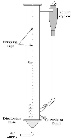
Figure 1. Schematic view of the experimental setup. P1, P2, … are sampling taps.

Table 1. Properties for particles.

of these parameters is cross average diagonal line

(CLave) which represents the average amount of similarity states between trajectories of the two

systems and the time that both systems stay

at-tuned. This parameter is defined as:

(3)

where P(l) is the number of diagonal line of

leng-th l.

Cross recurrence analysis was done for both normalized and non-normalized signals.

The signal was normalized as follows:

(4)

3. Experiments

Experiments were conducted in a column made of a Plexiglas pipe of 15 cm inner diameter and 2 m height. The experimental setup is schematically shown in Fig. 1. Air enters the column at ambient

temperature through a perforated plate distribu

-tor with 435 holes of 1.7 mm diameter arranged

in a 7 mm triangular pitch. Gas flow rate was mea

-sured and controlled by a mass flow controller (MFC). A cyclone was utilized to separate particles from air at high superficial velocities and return them back to the bed. The initial aspect ratio of solids in all experiments was one.

A pressure probe (Piezoresistive transducer,

Kobold Co., SEN-3248 B075) was used to mea

-sure pres-sure fluctuations of the bed at 10 cm above distributor. This probe had a response time of less than 1 ms. Absolute pressure fluctuations were recorded through a probe of 50 mm length and 4mm diameter with a fine mesh on its tip. The

measured signals were band-pass filtered (hard

-ware) at lower cut-off frequency of 0.1 and upper cut-off Nyquist frequency of 200 Hz. The pressure

transducer was connected to a 16-bit data acquisi

-tion board (Advantech 1712L). The filtered signals were then amplified with a gain of 100. In order to

satisfy the Nyquist criterion the sampling frequen

-cy for pressure fluctuation signals was adjusted to 400 Hz. The sampling frequency used in this work was 50 to 100 times more than the average cycle

frequency which is required for nonlinear evalua

-tion of the pressure fluctua-tions in bubbling fluid

-ized bed [23, 24].

(1)

𝑖𝑖− 𝑦𝑦 𝑗𝑗||) . 𝑖𝑖 = 1. … . 𝑁𝑁 ; 𝑗𝑗 = 1. … . 𝑀𝑀

(2)



 

 _N

l N

L l

l P

l lP CLave

1 () ) (

min ₍3)

Where P(l) is the number of diagonal line of length l.

Cross recurrence analysis was done for both normalized and non-normalized signals. The signal was normalized as follows:

S S i n S

S  _ (4)

3. Experiments

Experiments were conducted in a column made of a Plexiglas pipe of 15 cm inner diameter and 2 m height. The experimental setup is schematically shown in Fig. 1. Air enters the column at ambient temperature through a perforated plate distributor with 435 holes of 1.7 mm diameter arranged in a 7 mm triangular pitch. Gas flow rate was measured and controlled by a mass flow controller (MFC). A cyclone was utilized to separate particles from air at high superficial velocities and return them back to the bed. The initial aspect ratio of solids in all experiments was one.

A pressure probe (Piezoresistive transducer, Kobold Co., SEN-3248 B075) was used to measure pressure fluctuations of the bed at 10 cm above distributor. This probe had a response time of less than 1 ms. Absolute pressure fluctuations were recorded through a probe of 50 mm length and 4mm diameter with a fine mesh on its tip. The measured signals were band-pass filtered (hardware) at lower cut-off frequency of 0.1 and upper cut-off Nyquist frequency of 200 Hz. The pressure transducer was connected to a 16-bit data acquisition board (Advantech 1712L). The filtered signals were then amplified with a gain of 100. In order to satisfy the Nyquist criterion the sampling frequency for pressure fluctuation signals was adjusted to 400 Hz. The sampling frequency used in this work was 50 to 100 times more than the average cycle frequency

which is required for nonlinear evaluation of the pressure fluctuations in bubbling fluidized bed [23, 24].

Experiments were carried out with different Geldart B particles. For each sample 65535 data points were recorded which corresponding to about 164 seconds of sampling time. Size, minimum fluidization velocity (calculated using Wan and Yu Equation [25]) and velocity of onset of turbulent fluidization (calculated using standard deviation) of these particles are given in Table 1. Different superficial gas velocities in the range of 0.03 m/s to 1.2 m/s were used in the tests.

4. Result and Discussion

4.1 Cross recurrence plot

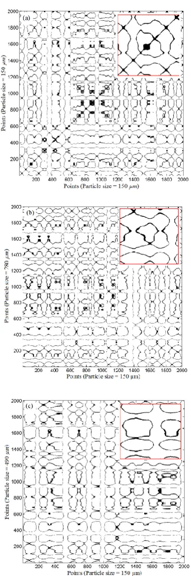
Hydrodynamics of fluidized beds could also be studied by the CRP method. The CRP of normalized pressure fluctuations of the fluidized bed considered in this work, is shown in Fig. 2 for different particle sizes at 0.3 m/s superficial gas velocity. Here, pressure fluctuation of the bed of 150 µm particles was considered as the reference signal. Radius threshold ε=0.01 and 2000 data points as the epoch length were used to construct the cross recurrence matrix. The CRP of the fluidized bed system with the same particle size (150 µm) and the same superficial gas velocity (0.3 m/s) is shown in Fig. 2(a). As mentioned previously, the CRP becomes a RP when two identical signals are used in Eq. (2). As expected, the LOI (line of identity) or main diagonal line of RP are completely seen in this figure. Fig. 2(b) demonstrates the CRP of pressure fluctuations of two different states of the bed. While the first signal is measured at particle size of 150 µm and superficial gas velocity of 0.3 m/s, the second signal is obtained from the bed of 280 µm particles and 0.3 m/s superficial gas velocity. It can be seen in this figure that the LOI is

Fig. 1 Schematic view of the experimental setup. P1, P2, … are sampling taps.

Mean particle

size (µm) (kg/mDensity 3₎ Umf (m/s) Uc (m/s)

150 2640 0.029 0.9

280 2640 0.059 1.1

490 2640 0.182 1.3

Experiments were carried out with different Geldart B particles. For each sample 65535 data points were recorded which corresponding to

about 164 seconds of sampling time. Size, mini

-mum fluidization velocity (calculated using Wan and Yu Equation [25]) and velocity of onset of turbulent fluidization (calculated using standard deviation) of these particles are given in Table 1. Different superficial gas velocities in the range of 0.03 m/s to 1.2 m/s were used in the tests.

4. Result and Discussion

4.1 Cross recurrence plot

Hydrodynamics of fluidized beds could also be

studied by the CRP method. The CRP of normal

-ized pressure fluctuations of the fluid-ized bed

considered in this work, is shown in Fig. 2 for dif

(4)

-56 H. Ziaei-Halimejani et al. / Journal of Chemical and Petroleum Engineering, 50 (2), Feb. 2017 / 53-60

13

14

15

Fig. 2 Cross recurrence plots pressure fluctuations of different states of the fluidized bed with different particle size at 0.3 m/s superficial gas velocity; (a) both 150 µm, (b) 150 µm and 280 µm, and (c) 150 µm and 490 µm. All plots were drawn using 2000 points of normalized signals and threshold of 0.08.

Figure 2. Cross recurrence plots pressure fluctuations of different states of the fluidized bed with different particle size at 0.3 m/s superficial gas velocity; (a) both 150 µm, (b) 150 µm and 280 µm, and (c) 150 µm and 490 µm. All plots were drawn using 2000 points of normalized signals and threshold of 0.08.

locity. Here, pressure fluctuation of the bed of 150

µm particles was considered as the reference sig

-nal. Radius threshold ε=0.01 and 2000 data points as the epoch length were used to construct the cross recurrence matrix. The CRP of the fluidized bed system with the same particle size (150 µm) and the same superficial gas velocity (0.3 m/s) is shown in Fig. 2(a). As mentioned previously, the CRP becomes a RP when two identical signals are

used in Eq. (2). As expected, the LOI (line of iden

-tity) or main diagonal line of RP are completely seen in this figure. Fig. 2(b) demonstrates the CRP of pressure fluctuations of two different states of

the bed. While the first signal is measured at par

-ticle size of 150 µm and superficial gas velocity of

0.3 m/s, the second signal is obtained from the bed

of 280 µm particles and 0.3 m/s superficial gas velocity. It can be seen in this figure that the LOI is disrupted and density of diagonal structures is less than in the RP. Fig. 2(c) shows the CRP of the bed with 150 µm and 490 µm particles. There is no pattern similar to the RP in this figure. Therefore,

it can be concluded that the CRP can detect hydro

-dynamic similarities and differences between two states of the bed. It can be seen in Fig. 2 that single dots are rarely present in the CRP of the fluidized

bed which demonstrates their non-stochastic na

-ture. Therefore, the fluidized bed behaves between

stochastic (chaotic) and predictable (periodic sys

-tem as a regular one) sys-tems. This result has also

been proven by recurrence analysis and it has been confirmed that dynamical behavior of fluidized beds is placed between stochastic and predictable systems [16].

4.2 Cross Recurrence Quantification Analysis

Input parameters (i.e., embedding dimension, time

delay, minimum length of diagonal line and radius

threshold) and length of epoch should be specified for analyzing the pressure signals of fluidized beds by CRQA. Prior to parameter selection, the length of epoch (N) for the CRQA calculations should be discussed. The effect of number of data points has been investigated in Fig. 3 and it was concluded that CRQA variable studied in this work do not change considerably for N bigger than 2000. This shows that CRP method gives useful information with low amounts of data, concluding that it is a

powerful and easy method for fluidized bed analy

-sis. Effect of changes in Embedding dimension and

time delay parameters were studied in this work but there were not radical differences in the re -sults. Therefore, embedding dimension of 2 and

(5)

quantitative parameters that can reveal changes

in particle size and superficial gas velocity was ex

-ploited. Cross average diagonal line of CRP of two time series with different superficial gas veloci

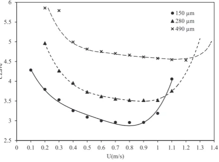
-ties is shown in Fig. 4. As can be seen in this figure, when data are not normalized, CLave changes with changing in the superficial gas velocity. In fact,

CLave decreases with increasing the superficial gas velocity since decreasing the attunement time

of two time series results in smaller CLave. Never

-theless, the CLave increases at higher gas veloci -ties. This change in the trend occurs at 0.8-0.9 m/s,

1.0-1.1 m/s and 1.2-1.3 m/s, respectively, for 150

µm, 280 µm and 490 µm particles. These veloci

-ties coincide with the transition from bubbling to turbulent fluidization regime. In fact, by increasing the superficial gas velocity in the bubbling regime,

bubbles (macro-structures) increase in the bed

(i.e., more heterogeneity) which results in decreas

-ing similarities of the two time series. This trend continues until the largest possible bubbles are formed in the bed, i.e., at the onset of turbulent flu

-idization. On the other words, CLave decreases

be-cause of decreasing attunement time of the system

state with reference signal. Beyond this velocity, bubbles (macro structures) transform into voids

(meso structures) and the share of macro struc-tures decreases in the hydrodynamics of the bed after transition to turbulent regime. On the other

words, dynamics of system changes and CLave

in-creases while velocity transition is occurred. In fact, the fluidized bed in the turbulent regime is

more homogeneous than in the bubbling regime.

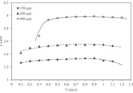
Sensitivity of CRQA parameters to change in the superficial gas velocity can be decreased by nor

-malizing the signals. Fig. 5 shows CLave of CRP be

-tween two states of the fluidized bed as a function

of superficial gas velocity using normalized pres

-sure fluctuations. In this figure, pres-sure fluctua -tions signal at U=0.9 m/s (as specified with dash line) was considered as the reference. It can be seen

in Fig. 5 that CLave of normalized signals change very gradually against superficial gas velocity. This demonstrates that this parameter is not sensitive to small variations of superficial gas velocity.

Effect of particle size on CRQA of pressure fluc

-tuations of fluidized bed was also investigated in

this work. Fig. 6 shows the variation of CLave as a

function of particle size at various gas velocities. Normalized pressure fluctuations of the bed of 150 µm particles were considered as the reference

signal. It can be seen in this figure that CLave

de-creases with increasing the particle size. The CLave

at 150 µm particle size is related to attunement

time of the system (obtained from the RP). CLave

16

Fig. 3 Cross average diagonal line of cross recurrence plot of different states within the fluidized bed as a function of epoch length. Pressure fluctuations of the fluidized bed of size 150 µm

particles were considered as the reference. U=0.5 m/s; ε=0.08 and ε=0.01 are considered for

normalized signal and non-normalized signal respectively. 3

3.1 3.2 3.3 3.4 3.5 3.6 3.7 3.8 3.9 4

0 400 800 1200 1600 2000 2400 2800 3200

CLa

ve

Epoch Length

280 µm-Normalized 280 µm-Non-normalized

Figure 3. Cross average diagonal line of cross recurrence plot of different states within the fluidized bed as a function of epoch length. Pressure fluctuations of the fluidized bed of size 150 µm particles were considered as the reference. U=0.5 m/s; ε=0.08 and ε=0.01 are considered for normal -ized signal and non-normal-ized signal respectively.

17

Fig. 4 Cross average diagonal line of cross recurrence plot of two states of the bed as a function of superficial gas velocity. Pressure fluctuations at U/Umf=1.5 is considered as the

reference signal. Epoch length= 2000 points, ε=0.01, and total length of time series= 65535 points. Signal is non-normalized.

2.5 3 3.5 4 4.5 5 5.5 6

0 0.1 0.2 0.3 0.4 0.5 0.6 0.7 0.8 0.9 1 1.1 1.2 1.3 1.4

CLa

ve

U(m/s)

150 µm 280 µm 490 µm

Figure 4. Cross average diagonal line of cross recurrence plot of two states of the bed as a function of superficial gas velocity. Pressure fluctuations at U/Umf=1.5 is considered as the reference signal. Epoch length=2000 points, ε=0.01, and total length of time series=65535 points. Signal is non-normalized.

length of diagonal line is (Lmin) 2 [19, 26, 27]. Ac

-cordingly, the optimum values of minimal length of diagonal lines have been chosen to be 2. The last input parameter is the radius threshold (ε), which determines the number of points appeared in the

cross recurrence plot. In this work, the suitable ra

-dius threshold, based on the method proposed by Webber and Zbilut [28], was obtained ε=0.01 for non-normalized and ε=0.08 for normalized signal.

To explore the ability of CRQA in detecting

(6)

5. Conclusion

CRQA method is a powerful tool to online detection of hydrodynamic status of a gas-solid fluidized bed. CRP of pressure fluctuation of the fluidized bed at various experimental conditions was obtained and the bed hydrodynamics changes were detected by cross average diagonal line. It was concluded that in the bubbling regime of fluidization, average

similarities of the systems decrease with increas

-ing the superficial gas velocity. However, cross av

-erage diagonal line increases in the turbulent

re-gime which indicates that the bed becomes more homogeneous in this condition. It was shown that cross average diagonal line of normalized signal is

not sensitive to changes in the superficial gas ve

-locity which is beneficial to detect the changes in particle size. Also, it was shown that cross average

diagonal line can detect the change of mean par

-ticle size in the bed and it varies significantly even if the signal is normalized.

Nomenclature

18

Fig. 5 Cross average diagonal line of cross recurrence plot of two systems as a function of superficial gas velocity. Pressure fluctuations at superficial gas velocity 0.9 m/s is considered as the reference signal. Epoch length= 2000 points, ε=0.08, total length of time series= 65535 points. Signal is normalized.

3 3.2 3.4 3.6 3.8 4 4.2

0 0.1 0.2 0.3 0.4 0.5 0.6 0.7 0.8 0.9 1 1.1 1.2 1.3

CLa

ve

U (m/s)

150 µm 280 µm 490 µm

Figure 5. Cross average diagonal line of cross recurrence plot of two systems as a function of superficial gas veloc -ity. Pressure fluctuations at superficial gas velocity 0.9 m/s is considered as the reference signal. Epoch length=2000 points, ε=0.08, total length of time series=65535 points. Signal is normalized.

Figure 6. Cross average diagonal line of CRP between two states as a function of particle size. In all cases, state with particle size 150 µm is considered as the reference. Epoch Length=2000 points, total length of time series=65535, ε=0.08. Signal is normalized.

19

Fig. 6 Cross average diagonal line of CRP between two states as a function of particle size. In all cases, state with particle size 150 µm is considered as the reference. Epoch Length= 2000 points, total length of time series=65535, ε=0.08. Signal is normalized.

2.9 2.95 3 3.05 3.1 3.15 3.2 3.25 3.3 3.35 3.4

150 280 490

CLa

ve

Particle size of second signal 0.5 m/s

0.9 m/s

of the system with 280 µm particle size is related to attunement time of CRP between two states of the system with different particle sizes (150 µm as reference state and 280 µm as the evaluating one) and the same superficial gas velocity. It can be seen

that CLave at 280 µm is slightly less than that one at 150 µm, but the difference is not meaningful.

When particle size increases to 600 µm, change of

CLave is considerable. This shows that CLave can

detect particle size changes in fluidized bed.

CR Cross recurrence matrix between two phase _{space trajectories}

CR_ij Cross recurrence point CRP Cross recurrence plot

CRQA Cross recurrence quantification analysis Clave Cross average diagonal line

DM Distance matrix between phase space vectors i,j Indices

Lmin Minimum diagonal line length L Diagonal line length

M Embedding dimension

M Number of data points for second signal

N Number of data points for first signal or refer -ence signal