Max Planck Institute for Demographic Research Konrad-Zuse Str. 1, D-18057 Rostock·GERMANY www.demographic-research.org
DEMOGRAPHIC RESEARCH
VOLUME 23, ARTICLE 19, PAGES 531-548
PUBLISHED 07 SEPTEMBER 2010
http://www.demographic-research.org/Volumes/Vol23/19/ DOI: 10.4054/DemRes.2010.23.19
Formal Relationships 10
Reproductive value, the stable stage
distribution, and the sensitivity of the
population growth rate to changes in vital rates
Hal Caswell
This article is part of the Special Collection “Formal Relationships”. Guest Editors are Joshua R. Goldstein and James W. Vaupel.
c
°2010 Hal Caswell.
A Background: Stable age theory 533
B Background: Matrix population models 533
C Background: Matrix calculus 534
2 Age-classified populations 534
2.1 The relationship 534
2.2 Derivation 535
2.2.1 Changes in mortality 535
2.2.2 Changes in fertility 537
2.3 History and perspectives 537
3 Stage-classified populations 539
3.1 The relationship 539
3.2 Derivation 539
3.3 Age-classified models as a special case 540
3.4 Sensitivity to lower-level demographic parameters 541
3.5 History, perspective, and generalizations 542
4 Sensitivity of growth rate via matrix calculus 542
4.1 The relationship 542
4.2 Derivation 543
4.3 History and extensions 543
5 Conclusion 544
6 Acknowledgments 544
Reproductive value, the stable stage distribution, and the sensitivity
of the population growth rate to changes in vital rates
Hal Caswell1
Abstract
The population growth rate, or intrinsic rate of increase, is the rate of growth that will be achieved by a population with fixed vital rates. The sensitivity of population growth rate to changes in the vital rates can be written in terms of the stable stage or age distribution and the reproductive value distribution. If the vital rate measures the rate of production of one type of individual by another, then the sensitivity of growth rate is proportional to the reproductive value of the destination type and the abundance in the stable stage distribution of the source type. This formal relationship exists in three forms: one for age-classified populations, a second that applies to stage- or age-classified populations, and a third that uses matrix calculus. Each uses a different set of formal demographic techniques; together they provide a relationship that beautifully spans different types of demographic models.
1. Introduction
A population subject to time-invariant vital rates will (with a few exceptions not of interest here) converge to a stable structure and grow exponentially at a constant rate (the population growth rate, or intrinsic rate of increase). The calculation of the population growth rate from the vital rates is one of the most important accomplishments of formal demography (Sharpe and Lotka 1911: Euler’s anticipation of the result in 1760 was not rediscovered until 1970).
If the vital rates change, so will the population growth rate. Perturbation analysis calculates the sensitivity of the growth rate to such changes, and may be useful for several reasons:
(i) To predict the effects of future changes, or to understand the effect of past changes, in the vital rates.
(ii) To determine the fitness consequences of genetic variation in demographic characteristics, and predict the evolutionary outcome of natural selection.
(iii) To compare the results of population policies or, in ecological contexts, of conservation or management strategies.
A Background: Stable age theory
The following relationships from age-classified stable population theory are used in deriving the relationships (1) and (2).
µ(x) mortality rate
(A-1)
`(x) = exp
µ −
Z x
0
µ(a)da 
survivorship (A-2)
m(x) maternity function
(A-3)
1 =
Z ∞
0
e−ra`(a)m(a)da Euler-Lotka equation forr
(A-4)
c(x) = e −rx`(x) Z ∞
0
e−ra`(a)da
stable age distribution (A-5)
v(x) = e
rx `(x)
Z ∞
x
e−ra`(a)m(a)da reproductive value
(A-6)
b=
·Z ∞
0
e−ra`(a)da ¸−1 birth rate (A-7) ¯ A= Z ∞ 0
ae−ra`(a)m(a)da mean age of reproduction
(A-8)
B Background: Matrix population models
The relationship (24) for stage-classified models is based on a matrix population model, using the following results regarding eigenvalues, eigenvectors, and stable population theory.
n(t) population vector at timet
(B-1)
n(t+ 1) =An(t) projection equation (B-2)
A=¡ aij ¢
population projection matrix (B-3)
λ= maxeig(A) population growth rate (B-4)
Aw=λw stable stage distributionw
(B-5)
vTA=λvT reproductive value vectorv
C Background: Matrix calculus
This section collects results from matrix calculus (Magnus and Neudecker 1988), used in deriving the formal relationship (37).
dy
dxT =
µ dyi dxj
derivative of vectoryw.r.t. vectorx
(C-1)
vec
µ a b c d
=¡ a c b d ¢T
vec operator: stacks columns into a vector (C-2)
dvecY
dvecTX derivative of matrixYw.r.t. matrixX (C-3)
dy=Qx=⇒ dy
dxT =Q First identification theorem (C-4)
vec(ABC) = (CT⊗A)vecB Roth’s theorem (C-5)
dy
dzT =
dy
dxT
dx
dzT vector chain rule
(C-6)
2. Age-classified populations
The population growth raterin an age-classified model is calculated from the Euler-Lotka equation (A-4) as a function of the age schedules of mortality and fertility (Section A).
2.1 The relationship
The sensitivities ofrto changes in mortality and fertility at agexare
dr dµ(x) =
−c(x)v(x)
bA¯ (1)
dr dm(x) =
c(x)
bA¯ (2)
of rto a change in fertility at age xis proportional to the stable age distribution (and the reproductive value at age 0, which, equals 1; see Section 3.). The proportionality constant in each case is the inverse of the product of the birth rate and the mean age of reproduction.
2.2 Derivation
This perturbation analysis of r relies on implicit differentiation of the Euler-Lotka equation (A-4). Let us introduce a perturbation parameterθ to measure the change in mortality or fertility at a specified age.
Writing survival, fertility, andras functions ofθgives the Euler-Lotka equation
(3) 1 =
Z ∞
0
e−r(θ)a`(θ, a)m(θ, a)da.
Differentiating both sides of (3) with respect toθgives
0 = −dr(θ) dθ
Z ∞
0
ae−r(θ)a`(θ, a)m(θ, a)da
+
Z ∞
0
e−r(θ)ad`(θ, a)
dθ m(θ, a)da
+
Z ∞
0
e−r(θ)a`(θ, a)dm(θ, a) dθ da. (4)
Solving (4) fordr/dθgives
(5) dr(θ)
dθ = 1 ¯ A ∞ Z 0
e−r(θ)ad`(θ, a)
dθ m(θ, a)da+
∞
Z
0
e−r(θ)a`(θ, a)dm(θ, a)
dθ da
whereA¯is the mean age of reproduction in the stable population (A-8).
2.2.1 Changes in mortality
If the perturbation affects mortality at agex, we write
whereδ(x)is the unit impulse function.2 The sensitivity ofrtoµ(x)is obtained as the
derivative ofrwith respect toθ, evaluated atθ= 0,
(11) dr
dµ(x) =
dr dθ ¯ ¯ ¯ ¯ θ=0 .
Because only mortality is affected byθ
dm(θ, a)
dθ = 0
(12)
dµ(θ, a)
dθ = δ(a−x). (13)
From (A-2),
d`(θ, a)
dθ = −e
−Ra 0 µ(θ,s)ds
Z a
0
δ(a−x)da (14)
= −`(θ, a)H(a−x). (15)
Substituting into (5) and evaluating atθ= 0gives
(16) dr
dµ(x) =
−1 ¯
A µZ ∞
x
e−ra`(a)m(a)da 
.
2The unit impulse function, or Dirac delta function, is a generalized function defined by
δ(x) = 0 x6= 0 (7)
Z ∞
−∞
δ(s)ds = 1.
(8)
The unit impulse is used in signal processing (e.g., Kamen and Heck 1997: p. 7) to represent the limit of a perturbation of unit strength applied over a shorter and shorter time interval. It’s most useful properties in our application are
(9)
Z∞
−∞
δ(a−x)f(a)da=f(x)
and
(10)
Z x
−∞
δ(s)ds=H(x)
The integral in (16) is close to the reproductive valuev(x)(A-6); specifically,
(17)
Z ∞
x
e−ra`(a)m(a)da=`(x)e−rxv(x).
However, from (A-5) and (A-7), `(x)e−rx = c(x)/b. Making these substitutions into
(16) gives the formal relationship (1).
2.2.2 Changes in fertility
If the perturbation affects fertility at agex, we write
(18) m(θ, a) =m(0, a) +θδ(a−x).
Because only fertility is affected byθ,dµ(θ, a)/dθ = 0anddm(θ, a)/dθ =δ(a−x). Substituting these into (5) and evaluating the result atθ= 0gives
(19) dr
dm(x)= 1
¯
A ³
e−rx`(x)´.
From (A-5) and (A-7) it can be seen that the numerator is c(x)/b, which leads to the formal relationship (2).
2.3 History and perspectives
Hamilton (1966) obtained the relationship (16) in an analysis of the evolution of senescence. From (16) and (2) it is apparent that (providedr≥0) the magnitudes of the sensitivities ofrto mortality and fertility decline with age. These sensitivities measure the selection gradients on age-specific mortality and fertility. Thus Hamilton concluded that the strength of selection against deleterious mutations would decline with their age of action, that small positive effects at early ages could easily compensate for much larger negative effects at later ages, and that the evolution of senescence was therefore inevitable. In the years that followed Hamilton’s paper, several other authors developed perturbation analysis for r, using related methods. Demetrius (1969) used a discrete age-classified model, and Emlen (1970) used Hamilton’s results to derive the dynamics of gene frequencies resulting from the selection gradients on age-specific survival and fertility.
appearance of reproductive value in the sensitivity ofr to mortality. Goodman (1971) was apparently the first to note that the sensitivities ofrto mortality and fertility could be expressed in terms of the stable age distribution and reproductive value. Arthur (1984) presented an approach based on functional differentiation; it would be interesting to explore the connections between that approach and the matrix calculus methods in Section 4.
When Hamilton’s paper appeared in 1966, it was regarded as difficult and esoteric, but it had a great impact. It provided the analytical machinery for examining trade-offs between opposing demographic traits (“antagonistic pleiotropy;" Williams 1957; Rose 1991; Charlesworth 1994). These ideas are fundamental to the analysis of human aging (e.g., Rose 1991; Wachter and Finch Washington, D.C.: National Academy Press; Carey and Tuljapurkar 2003; Baudisch 2005) and, more generally, the analysis of life history evolution in humans and other species (e.g., Charlesworth 1994; Stearns 1992). In the most recent overview of evolutionary biodemography (Vaupel 2010), Hamilton’s paper is still one of the foundations of evolutionary life history theory; in the most recent overview of evolutionary biodemography (Vaupel 2010), the paper is one of the first citations.
Hamilton’s conclusions about the inevitability of senescence depend on the nature of the perturbations described here by (6) and (18) — that is, additive perturbations to mortality or fertility, respectively. Baudisch (2005; 2008) has pointed out that traits leading to other kinds of perturbations would experience different patterns of selection pressure with age. She examined proportional changes in mortality,
(20) dr
dlogµ(x) =µ(x)
dr dµ(x),
additive changes in survivalp(x) =e−µ(x),
(21) dr
dp(x)=− 1
p(x)
dr dµ(x),
and proportional changes in survival
(22) dr
dlogp(x) =−
dr dµ(x).
One could also include proportional changes in fertility
(23) dr
dlogm(x) =m(x)
There is no a priori reason that such traits should not arise in the course of evolution, but they lead to very different conclusions about senescence. In particular, the magnitudes of (20), (21), and (23) may increase, rather than decrease, with age (Baudisch 2005), so Hamilton’s conclusion does not apply to such perturbations.
3. Stage-classified populations
Implicit in Hamilton’s analysis is the assumption that the vital rates are functions of age. In many cases, they are not. In humans, characteristics such as economic, marital, or health status, or spatial location, may provide important information in addition to age. In other species, the vital rates depend on developmental stage or size more than on age. Such populations are described by stage-classified demographic models, of which the age-classified theory is a special case.
Stage-classified demography can be analyzed using matrix population models (Leslie 1945; Caswell 2001); see Section B. The discrete-time population growth rateλis the dominant eigenvalue of the population projection matrix A(guaranteed to be real and positive by the Perron-Frobenius theorem; Caswell 2001). The effects of perturbations on population growth can be approached by looking for the sensitivity of an eigenvalue to changes in the entries of a matrix.
3.1 The relationship
The sensitivity ofλto a change in the entryaijofAis (Caswell 1978)
(24) ∂λ
∂aij
=viwj
vTw,
where the stable stage distributionw and the reproductive value vectorv are the right and left eigenvectors ofA. The entryaij measures the per-capita production of stagei
by stagej. The effect of a change inaij is proportional to the reproductive value of the
destination stage and to the abundance of the origin stage in the stable population. This is a generalization of the relationships (1) and (2) obtained from Hamilton’s analysis.
3.2 Derivation
A+ ∆A. This will result in perturbations ofλand ofw, which must satisfy
(25) (A+ ∆A) (w+ ∆w) = (λ+ ∆λ)(w+ ∆w).
Expanding the products, setting second order terms to zero, and remembering thatAw=
λwgives
(26) A(∆w) + (∆A)w=λ(∆w) + (∆λ)w.
Multiply on the left byvTand simplify to obtain
(27) (∆λ)vTw=vT(∆A)w.
If the perturbation affects only one entry, for exampleaij, ofA, then
(28) ∆λ= viwj(∆aij)
vTw .
Dividing both sides by∆aijand taking the limit as∆aij→0gives the relationship (24).
3.3 Age-classified models as a special case
To compare (24) with Hamilton’s results (1) and (2), consider an age-classified matrix (a Leslie matrix) with fertilities Fi in the first row, survival probabilities Pi on the
subdiagonal, and zeros elsewhere (Leslie 1945; Keyfitz 1968). In this case (24) simplifies to
∂λ ∂Pi
= vi+1wi
vTw
(29)
∂λ ∂Fi
= v1wi
vTw.
(30)
3.4 Sensitivity to lower-level demographic parameters
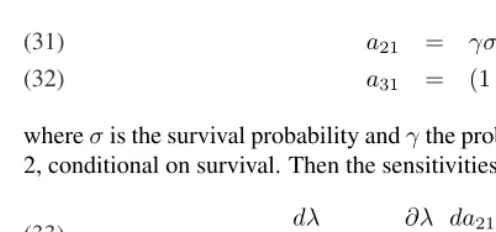
Figure 1: An example of lower-level parameters appearing in a portion of a life cycle.
1
2
3 a21 = σγ
a31 = σ(1−γ)
Note: Individuals in stage 1 survive with probabilityσ, and, conditional on survival, move to stage 2 with probabilityγand to stage 3 with probability1−γ.
The entries ofAare often functions of other, lower-level parameters. The sensitivity ofλto these parameters is obtained by the chain rule. For example, suppose that stage 1 may contribute individuals to stages 2 or 3 (Figure 1). Write the transition probabilities as
a21 = γσ
(31)
a31 = (1−γ)σ
(32)
whereσis the survival probability andγthe probability that the individual moves to stage 2, conditional on survival. Then the sensitivities ofλtoγand toσare given by
dλ dσ =
∂λ ∂a21
da21 dσ +
∂λ ∂a31
da31 dσ
(33)
= w1[γv2+ (1−γ)v3]
vTw
(34)
dλ dγ =
∂λ ∂a21
da21 dγ +
∂λ ∂a31
da31 dγ
(35)
= σw1(v2−v3)
vTw .
The sensitivity to survival is proportional to the weighted average of the reproductive values of the destination stages, and the sensitivity to the transition probability γ is proportional to the difference in reproductive value between the destination stages.
3.5 History, perspective, and generalizations
I first encountered this perturbation expansion in the proceedings of an engineering conference (Desoer 1967). Eigenvalue perturbations were of particular interest to engineers in the 1960s as part of a shift from frequency-domain methods to state-space methods in the study of linear systems (Zadeh and Desoer 1963). However, the result dates back to Jacobi (1846), and has been independently rediscovered many times (e.g., Faddeev 1959; Papoulis 1966; Franklin 1968). This perturbation approach has been extended to many other sensitivity problems, including the sensitivity of subdominant eigenvalues and transient behavior, of growth rates in periodic and stochastic environments, of the eigenvectors, and of the spreading speed in biological or demographic invasions (see Caswell 2001: for reviews and references).
4. Sensitivity of growth rate via matrix calculus
Eq. (24) assumes that only a single entry ofAis perturbed, and derivatives with respect to other parameters must be assembled by summing the effects of those parameters on all the entries ofA, as in (36). A powerful alternative approach is to treatλas a scalar function ofA, andAas a matrix-valued function of a vector of lower-level parameters. The mathematical machinery of matrix calculus (Section C, Magnus and Neudecker 1988) makes it possible to do this.
4.1 The relationship
Suppose thatA is a function of a vectorθ, of dimension p×1, of parameters. The derivative ofλwith respect toθis
(37) dλ
dθT =
µ
wT⊗vT
vTw
¶ µ dvecA
dθT
¶ ,
where⊗denotes the Kronecker product. In this notation,dλ/dθT
is a1×pvector whose
4.2 Derivation
Begin by taking the differential of both sides of (B-5) to give
(38) (dA)w+A(dw) = (dλ)w+λ(dw).
where the differential of a matrix or vector is the matrix or vector containing the differentials of the elements. Multiply both sides on the left byvTand simplify to obtain
(39) (dλ)vTw=vT(dA)w
Next, apply the vec operator (C-2) to both sides of (39). Since the left side is a scalar, the vec operator has no effect. The right side is a product of three quantities, so Roth’s theorem (C-5) implies that
(40) dλ= w
T⊗vT
vTw dvecA
Equation (C-4) (the First Identification Theorem; Magnus and Neudecker 1985), implies that
(41) dλ
dvecTA = (w
T⊗vT).
Finally, the chain rule (C-6) gives us the formal relationship (37), for the sensitivity of
λto any vector of parameters. This generalizes the expression (24), but permits easy calculation of the derivatives without having to keep track of summations.
4.3 History and extensions
Modern versions of calculus for matrix equations date back to Dwyer and MacPhail (1948). Several different and not totally compatible approaches have been developed (Nel 1980). The approach adopted here was developed by Magnus and Neudecker (1985) See Magnus and Neudecker (1988) for a complete treatment, and Abadir and Magnus (2005) for a recent introduction).
stage-structured epidemic models (Klepac and Caswell 2010), and to transient dynamics (Caswell 2007).
5. Conclusion
The three versions of this formal relationship, equations (1 – 2), (24), and (37), use different analytical methods but agree in showing how the sensitivity of population growth rate can be written in terms of the stable stage distribution and the reproductive value. In general, the effect of a change in the rate at which individuals move from stagejto stage
iis proportional to the abundance of the origin stage (j) and the reproductive value of the destination stage (i). If a vital rate produces individuals with low reproductive value, or if few individuals are available to experience the change in the rate, the effect on population growth will be small.
In the age-dependent model, the sensitivity ofrto changes in fertility (2) appears to lack the dependence on the destination reproductive value; this is because the reproductive value at age 0 is 1. In the stage-dependent model, the reproductive value of the first stage (whatever kind of newborn individual that may represent) is explicitly present in the expression (30).
Each version of this formal relationship uses a different approach to perturbation analysis: implicit differentiation, perturbation expansion, or matrix calculus. Of course, these methods are all related, but each of them is particularly appropriate in its own situations. As a result, perturbation analysis in demography now extends far beyond the population growth rate (e.g., Caswell 2001; 2008; 2009b).
6. Acknowledgments
References
Abadir, K.M. and Magnus, J.R. (2005). Matrix algebra. Econometric exercises 1. Cambridge, United Kingdom: Cambridge University Press.
Arthur, B.W. (1984). The analysis of linkages in demographic theory.Demography21(1): 109–128.doi:10.2307/2061031.
Baudisch, A. (2005). Hamilton’s indicators of the force of selection. Proceedings of the National Academy of Sciences102(23): 8263–8268. doi:10.1073/pnas.0502155102. Baudisch, A. (2008). Inevitable aging? Contributions to evolutionary-demographic
theory. Berlin, Germany: Springer-Verlag.
Carey, J.R. and Tuljapurkar, S. (2003). Life span: evolutionary, ecological, and demographic perspectives. Population and Development ReviewSupplement 29: New York, NY: Population Council.
Caswell, H. (1978). A general formula for the sensitivity of population growth rate to changes in life history parameters. Theoretical Population Biology 14(2): 215–230. doi:10.1016/0040-5809(78)90025-4.
Caswell, H. (2001). Matrix population models: Construction, analysis, and interpretation. Second edition. Sunderland, Massachusetts, USA: Sinauer Associates. Caswell, H. (2006). Applications of Markov chains in demography. In: A.N. Langville
and W.J. Stewart (eds.) MAM2006: Markov Anniversary Meeting. Raleigh, North Carolina, USA: Boson Books: 319–334.
Caswell, H. (2007). Sensitivity analysis of transient population dynamics.Ecology Letters
10(1): 1–15.doi:10.1111/j.1461-0248.2006.01001.x.
Caswell, H. (2008). Perturbation analysis of nonlinear matrix population models.
Demographic Research18(3): 59–116.doi:10.4054/DemRes.2008.18.3.
Caswell, H. (2009a). Sensitivity and elasticity of density-dependent population models. Journal of Difference Equations and Applications 15(4): 349–369. doi:10.1080/10236190802282669.
Caswell, H. (2009b). Stage, age, and individual stochasticity in demography. Oikos
118(12): 1763–1782.doi:10.1111/j.1600-0706.2009.17620.x.
Charlesworth, B. (1994). Evolution in age-structured populations. Second edition. Cambridge, United Kingdom: Cambridge University Press.
Demetrius, L. (1969). The sensitivity of population growth rate to perturbations
doi:10.1016/0025-5564(69)90009-1.
Desoer, C.A. (1967). Perturbations of eigenvalues and eigenvectors of a network. Urbana, Illinois, USA: University of Illinois: 8–11. Fifth Annual Allerton Conference on Circuit and System Theory.
Dwyer, P.S. and MacPhail, M.S. (1948). Symbolic matrix derivatives. Annals of Mathematical Statistics19: 517–534.doi:10.1214/aoms/1177730148.
Emlen, J.M. (1970). Age specificity and ecological theory. Ecology 51(4): 588–601. doi:10.2307/1934039.
Euler, L. (1970). A general investigation into the mortality and multiplication of the human species. Theoretical Population Biology1(3): 307–314 (Originally published 1760).doi:10.1016/0040-5809(70)90048-1.
Faddeev, D.K. (1959). The conditionality of matrices (“ob obuslovlennosti matrits”). Matematicheskii institut Steklov: 387–391. Trudy No. 53.
Faddeev, D.K. and Faddeeva, V.N. (1963).Computational methods of linear algebra. San Francisco, California, USA: W. H. Freeman.
Franklin, J.N. (1968).Matrix theory. Englewood Cliffs, New Jersey, USA: Prentice-Hall. Goodman, L.A. (1971). On the sensitivity of the intrinsic growth rate to changes in the age-specific birth and death rates. Theoretical Population Biology2(3): 339–354. doi:10.1016/0040-5809(71)90025-6.
Hamilton, W.D. (1966). The moulding of senescence by natural selection. Journal of Theoretical Biology12(1): 12–45.doi:10.1016/0022-5193(66)90184-6.
Jacobi, C.J.G. (1846). Über ein leichtes Verfahren, die in der Theorie der Säkularstörungen vorkommenden Gleichungen numerisch aufzulösen. Journal für reine und angewandte Mathematik30: 51–95.
Jenouvrier, S., Caswell, H., Barbraud, C., and Weimerskirch, H. (2010). Mating behavior, population growth and the operational sex ratio: a periodic two-sex model approach.
American Naturalist175(6): 739–752.doi:10.1086/652436.
Kamen, E.W. and Heck, B.S. (1997).Fundamentals of signals and systems. Upper Saddle River, New Jersey, USA: Prentice Hall.
Keyfitz, N. (1968). Introduction to the mathematics of population. Reading, Massachusetts, USA: Addison-Wesley.
Klepac, P. and Caswell, H. (2010). The stage-structured epidemic: linking disease and demography with a multi-state matrix model approach. Theoretical Ecology
doi:10.1007/s12080-010-0079-8.
Leslie, P.H. (1945). On the use of matrices in certain population mathematics.Biometrika
33(3): 183–212. doi:10.1093/biomet/33.3.183.
Magnus, J.R. and Neudecker, H. (1985). Matrix differential calculus with applications to simple, hadamard, and kronecker products. Journal of Mathematical Psychology
29(4): 474–492. doi:10.1016/0022-2496(85)90006-9.
Magnus, J.R. and Neudecker, H. (1988).Matrix differential calculus with applications in statistics and econometrics. New York, NY, USA: John Wiley & Sons.
Nel, D.G. (1980). On matrix differentiation in statistics.South African Statistical Journal
14: 137–193.
Papoulis, A. (1966). Perturbations of the natural frequencies and eigenvectors of a network.IEEE Transactions on Circuit TheoryCT-13(2): 188–195.
Roff, D.A. (1992). The evolution of life histories. New York, NY, USA: Chapman and Hall.
Rose, M.R. (1991). Evolutionary biology of aging. Oxford, United Kingdom: Oxford University Press.
Sharpe, F.R. and Lotka, A.J. (1911). A problem in age-distribution. Philosophical Magazine21: 435–438.doi:10.1080/14786440408637050.
Stearns, S.C. (1992). The evolution of life histories. Oxford, United Kingdom: Oxford University Press.
Vaupel, J.W. (2010). Biodemography of human ageing. Nature 464: 536–542. doi:10.1038/nature08984.
Verdy, A. and Caswell, H. (2008). Sensitivity analysis of reactive ecological
dynamics. Bulletin of Mathematical Biology 70(6): 1634–1659. doi:
10.1007/s11538-008-9312-7.
Wachter, K.W. and Finch, C.E. (Washington, D.C.: National Academy Press). Between Zeus and the salmon: the biodemography of longevity. 1997.
Williams, G.C. (1957). Pleiotropy, natural selection, and the evolution of senescence.
Evolution11: 398–411.