Effectivity of Hypergeometric Function Application in the Numerical Simulation of the Helicopter Rotor Blades Theory

Effectivity of Hypergeometric Function Application in the

Numerical Simulation of the Helicopter Rotor Blades Theory

Dragoljub Bekrić1,* _{- Časlav Mitrović} 1 _{- Dragan Cvetković} 2 _{- Aleksandar Bengin} 1 1 _{University of Belgrade, Faculty of Mechanical Engineering, Serbia} 2 _{Singidunum University, Faculty of Bussiness Information Science, Serbia}

Efficiency and justification of hypergeometric functions application in achieving simple formulas used in numerical simulation of helicopter rotor blades theory are presented in this paper.

Basic equations of stream field over helicopter rotor are formulated, their decomposition is made and mean induced velocity harmonics are integrally presented. Theoretical basis of hypergeometric function application in transformation of integral equations of k-bladed rotor average induced velocity into special functions follows. The necessary conditions for transformation hypergeometric functions into special functions are defined.

Variants of integral transformation of expressions obtained are presented by a numerical simulation and solutions are found. This approach to cecure the effectivity of hypergeometric function application in helicopter rotor blades theory by numerical simulation provides a synthetic method, which can be used to define helicopter k-bladed main rotor optimal characteristics.

© 2010 Journal of Mechanical Engineering. All rights reserved.

Keywords: hypergeometric functions, unsteady flow, numerical simulation, lifting line, free vortex model, helicopter rotor aerodynamics

0 BASIC ASSUMPTIONS AND MUTUAL RELATIONS

In practical rotor calculations based on disc theory it can be assumed that circulation along the supporting line is constant over blade azimuth angle. This assumption does not cause large differences in induced velocity computation

at small values of μ, and it significantly

simplifies the computation.

This assumption is applied only to induced velocities calculation which forms the basis for further determination of actual values of the angles of the attack blade section and variable circulation Γ ρ θ

(

ˆ,

)

which are necessary for rotor characteristics calculation.

Let the k-bladed rotor with diameter 2R

and center in origin of Cartesian system Oxyz be placed in an undisturbed flow field with velocity

V. The rotor is rotating around y-axis with angular velocityω. The direction of velocity V forms the arbitrary angle α with xz plane. The rotor blade is presented by a radial segment of supporting line with circulation varying with radius

(

)

0 R

ρ ≤ ≤ρ and with constant circulation over

azimuth angle θ.

It is assumed that free vortex elements separating from lifting line are moving in space

Oxyz along with particles of undisturbed flow

field forming vortex shade in the form of pitched spiral surface. Induced velocity V is calculated in arbitrary point of xz plane. That point is defined by polar coordinates: radius r and azimuth angle

ψ .

In order to simplify the calculation, dimensionless coefficients defined by the following expressions will be used:

2

; ; ; V

V

R R R

Γ ρ

Γ ρ

ω ω

= = =

; r r

r R

ρ

ρ)= = .

Induced velocity can be presented in following integral form [1]:

1 1

0 0

4 4

r p q

k k

v v d d

V r

∂Γ

ρ ρ

π π ∂ρ

= +

∫

Φ +

∫

Φ

(1)

where

( )

4 r

k r

v

V

Γ π = −

(2)

(

)

2 2 0

sin cos 1

2 cos

z p

x

L

d L L L

π _{ρ θ α}

Φ θ

π α

=

+

∫

)

(

)

2

0

cos 1

2 cos

z q

x

L

d L L L

π _α

Φ θ

π α

=

+

∫

(4)

and

(

cos 1 cos

)

sin sin ;

x

L = ρ) θ− ψ ρ− ) θ ψ

(

cos 1 sin

)

sin cos ;

z

L = ρ) θ− ψ ρ+ ) θ ψ

2

1 2 cos

L= +ρ) − ρ) θ .

Periodic functions (3) and (4) with period 2 have the following characteristics:

( )

( )

( )

( )

; ;

p p

q q

Φ ψ Φ ψ

Φ ψ Φ ψ

− =

− = − ₍₅₎

and consequently:

2 2

0 0

0.

pd qd

π π

Φ ψ = Φ ψ =

∫

∫

Therefore, the second term in expression (1) presents velocity field component symmetrical in regard to x-axis, and the third term presents velocity field component asymmetrical

in regard to x-axis. Let the velocity v be

presented in the form of Fourier series progression:

(

)

1

cos sin ,

r cn sn

n

v v ∞ v nψ v nψ

=

= +

∑

−

and coefficients determined as

2 0 2

0

1

cos ;

1 _sin

cn

sn

v v n d

v v n d

π

π

ψ ψ π

ψ ψ π

= =

∫

∫

₍₆₎

by use of Eq. (1).

By replacing t= +ψ ϕ Eq. (1) is

transformed on the basis of (5) and (6) into:

1 0

4 n

cn n

kk

v C d

V

α ∂Γ _ρ

π ∂ρ

= −

_∫

(7)

1 0

4 n

sn n

kk

v S d

r

α ∂Γ _ρ

π ∂ρ

= −

_∫

(8)

where

2 0

1 sin sin cos

2 1 cos cos

n

t nt

k dt

t

π

α

α

π α

= −

+

∫

₍₉₎

2 0 2

0

1 1_{sin sin ;}

1 1

cos .

n

n

C n d

L

S n d

L

π

π

ϕ ϕ θ

π

ϕ θ π

= =

∫

∫

₍₁₀₎

Integral (9) is calculated elementarily and integrals (10) are presented in form:

(

)

(

)

1 1

0

1 1

cos cos ;

n n n

C T T d

L

π

ϕ ϕ θ

π ⎡ − + ⎤

=

_∫

_⎣ − _⎦

(11)

(

)

0

2 1

cos .

n n

S T d

L

π

ϕ θ π

=

_∫

(12) In Eq. (12) Tn(cos ϕ) = cos nϕ is the

first order Chebyshev polynomial. Chebyshev polynomials are convenient because the second Eq. from (8) is excluded. Consequently from (1) and (12) it follows:

(

1 1

)

1 2

n n n

C = S ₋ −S ₊

(13) which correlates coefficients (7) and (8)

1 1 1

1

1 , 2

cn sn sn

r

v k v v

V α − kα +

⎛ ⎞

= _⎜ − _⎟

⎝ ⎠

where kα₁ is value kαnfor n=1.

From Eqs. (11) and (12) it follows that nuclei Cnand Snof integrals (9) and (10) are not dependent of parameters characterizing rotor working order. Integral (12) allows transformation into hypergoemetric function. It can be shown that integral (12) represents the solution of Gauss differential equation:

(

1

)

(

1

)

0

ξ −ξ η′′+_⎣⎡γ− α β+ + ξ η αβη⎤_⎦ ′− =

with boundary conditions defined by nucleus (12) in the form:

( )

( )

(

)

0 2

0 2m m 1

η η

= −

′ = + ₍₁₄₎

if

2_{; m; m 1; 1}

Consequently it follows that integral (12) represents hypergeometric function in form

(

2

)

2 1

2 , 1,1; ; 1

0; 1.

m

F m m

S ρ ρ

ρ

+

⎧− − + <

⎪ = ⎨

> ⎪⎩

) )

)

(15)

Hypergeometric function Fin expression

(15) is Legendre polynomial P_m for _{x= −1 2ρˆ}2_.

The calculation of nucleus (14) by using Legendre polynomial has the following form:

(

2

)

2 1

2 1 2 ; 1

0; 1.

m m

P

S ρ ρ

ρ

+

⎧− − <

⎪ = ⎨

> ⎪⎩

) )

)

(16)

For smaller values of index m expression (16) gives elementary expressions of the requested nuclei:

1

2 3

2 4

5

2 4 6

7

2; 2 4 ;

2 12 12 ;

2 24 60 40 .

S S S S

ρ

ρ ρ

ρ ρ ρ

= − = − + = − + −

= − + − +

)

) )

) ) )

(17)

Expression (16) can be rewritten in form

2 2 1

1

2 m

m m

S μ

μ μ

α ρ

+

=

= − −

∑

)

(18)

where

( ) (

)

( )

(

)

(

)

(

) (

)

2 ₂ 2 2

2 2

1 2 1 !!

2 1 1

2 ! 2 !

2 1 3

2 1 2 1

m m

m m

μ

μ μ

μ α

μ μ

μ

− − _{⎡ ⎤}

= _⎣ + − _⎦⋅

⎡ _{+ −} ⎤

⎣ ⎦

⎡ _{+ − −} ⎤

⎣ ⎦

K

K

where

(

2μ−1 !! 1 3 5

)

= ⋅ ⋅ ⋅⋅⋅

(

2μ−1

)

.

For nuclei calculation for large values of

index m it is convenient to use the recurrence

formula:

(

2

)

2 3 2 1 2 1

2 1 _{1 2 .}

1 1

m m m

m m

S S S

m ρ m

+ + −

+

= − −

+ ) + (19)

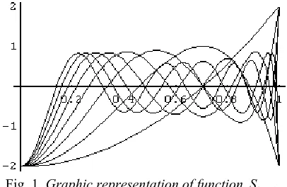
Graphic representations of function S_2m+1, for different m are shown in Fig. 1.

Fig. 1. Graphic representation of function S2m+1,

for different m

In addition to the practical results (17) to (19), a transformation of nucleusS2m+1in form

(16) gives the following integral representation of Legendre polynomial which contains Chebyshev polynomial in the form:

(

)

2 1

( )

0

1 cos

m m

d

P T p

l

π _θ

θ

π +

= −

_∫

where:

1 _{sin cos 1 ;}

2

p l

θ _θ

⎛ ⎞

= _⎜ − _⎟

⎝ ⎠

2

1 sin 2sin cos ;

2 2

l= + θ − θ θ

0≤ ≤θ π, 0, 1, 2,

m= _K

Since for ρ)>1 according to (18) nuclei

2m 1

S + are zero, formula (10) can be transformed

in the form:

(

)

2 1

2 1 2 1

0 cos

.

4 1 sin

m _r

s m m

k

v S d

r

α ∂Γ _ρ

π α ∂ρ

+

+ = +

+

⎛ ⎞

⎜ ⎟

⎝ ⎠

∫

₍₂₀₎

For the analytical solution the expression (20) can be rewritten in the form:

(

)

( )

2 _{1 1} 2 1

1 cos

4 1 sin

m

s m m

k

v P x d

r x

α ∂ _ρ

π α ∂

+ ₊

+

−

Γ =

+

⎛ ⎞

⎜ ⎟

⎝ ⎠

∫

(21) where _{x= −1 2ρ})2 _{and a partial derivative of the}

( )

0

h P x x μ μ μ

∂Γ ∂

∞

=

=

∑

(22) and taking into consideration that Legendre polynomial is orthogonal on the basis of equation (21) an analytical expression is obtained:

(

)

2 1 2 1

cos

2 1 1 sin

m m

s m

h k v

r m

α

π α

+

+

⎛ ⎞

= ⎜_⎜ ⎟_⎟

+ _⎝ + _{⎠ (23)}

which shows that coefficient v_{s m2 +1}is dependent only on one coefficient from expression (22), that

with index μ=m. By using Gauss

hypergeometric equations it can be shown, in a similar way to the transformation of Eq. (16), that integral (10) can be expressed by the following hypergeometric function:

( ) (

)

2

2

2 1 3 1

2

1 1

2 , ,1; ; 1

2 2

1 2 1 !!

2 ! _{; 1}

1 1 1

, , 2 1;

2 2

m

m

m m

S

F m m

m m

F m m m

ρ ρ

ρ

ρ

ρ

− −

−

=

− + + <

− −

⋅

>

− + +

⎧ ⎛ ⎞

⎜ ⎟

⎪ _{⎝ ⎠}

⎪

⎪⎛ ⎞

⎨⎜ ⎟

⎪⎜ ⎟

⎪⎜ _{⎛ ⎞}⎟

⎪⎜ ⎜ ⎟⎟

⎝ ⎠

⎝ ⎠

⎩

) )

)

)

)

(24) which can be transformed into the first and second order of Legendre functions.

(

)

( )

₍

₎

2 1 2 2

2 1 2

2 1 2 ; 1

1 4

2 1 ; 1.

m m m

m

P S

Q

ρ ρ

ρ ρ

π

−

−

⎧ − <

⎪⎪ = ⎨ −_⎪

− > ⎪⎩

) )

) )

(25) On the basis of expression (25) it is possible to achieve the following recurrence formula:

(

2

)

2 2 2 2 2

4

1 2

2 1

2 1 _.

2 1

m m m

m

S S S

m

m m

ρ

+ = − − −

+

− + )

(26) For a practical application of the calculation the function in expression (24) can be transformed into first and second order elliptic integrals by taking into consideration that they can be rewritten in the following form:

( )

( )

2 2

1 1

, ,1; ;

2 2 2

1 1_{, ,1; .}

2 2 2

K x F x

E x F x

π π

⎛ ⎞

= _{⎜ ⎟}

⎝ ⎠

⎛ ⎞

= _⎜− _⎟

⎝ ⎠ (27)

By replacing (27) intom=0 and m=1, the following equations are obtained:

( )

0

4

; 1

4 1

; 1

K S

K

ρ ρ

π

ρ

πρ ρ

⎧ _<

⎪⎪

= ⎨ _{⎛ ⎞} ⎪ _{⎜ ⎟ >}

⎪ _{⎝ ⎠}

⎩

) )

)

) )

(28)

and

( ) ( )

[

]

(

)

2

2

4

2 ; 1

4 1 1

2 2 1 ; 1

E K

S

E K

ρ ρ ρ

π

ρ ρ ρ

πρ ρ ρ

− <

=

− − >

⎧

⎪⎪

⎨

_⎡

_{⎛ ⎞}

_{⎛ ⎞⎤}

⎪

_⎢

_{⎜ ⎟}

_{⎜ ⎟}

_⎥

⎪ ⎣

⎝ ⎠

⎝ ⎠⎦

⎩

) ) )

) ) )

) ) )

(29)

Recurrence Eq. (26) with Eqs. (28) and (29) allows easy determination of nuclei S_2m for

every m greater than zero. Transformation of

(12) into (25) allows the following integral representation of the first and second order of Legendre function:

(

2

)

( )

1 2

2

1 2 m ; 0 1;

m

P x I x x

− − = ≤ < ₍₃₀₎

(

2

)

( )

( )

1 2

2

2 1 1 ; 1

2 m

m m

Q x π I x x

− − = − > ₍₃₁₎

where

( )

(

)

2 2

0

1

; 0,1, 2,

m m

d

I T p m

l

π _θ

π

=

_∫

= _K

and T2m

( )

p is the first order Chebyshev

polynomial with

(

)

1

cos 1

p x

l θ

= −

and

2

1 2 cos

l= +x − x θ .

(

2

)

(

2

)

1 2

1 2 1 2 ; 1

0; 1

m m

m

P P

C ρ ρ ρ

ρ

−

− − − <

=

>

⎧⎪ ⎨ ⎪⎩

) ) )

)

(32)

Nuclei C2m can be expressed as

hypergeometric functions by using assumptions:

(

)

2 2

2m 2 1, 1, 2;

C = − m Fρ) − +m m+ ρ) . ₍₃₃₎ For smaller values of index m elementary formulas are achieved:

2 2

2 2

4

2 4 6

6

2 4 6 8

8

2 ;

4 6 ;

6 24 20 ;

8 60 120 70 .

C C C C

ρ

ρ ρ

ρ ρ ρ

ρ ρ ρ ρ

= −

= − +

= − + −

= − + − +

)

) )

) ) )

) ) ) )

Nuclei C_nfor odd indices n=2m+1 can be transformed by using expressions (13) and (25) into the first and second order Jacobi functions which allows representation in the form of elliptic integrals. For smaller m it follows:

( )

( )

1

4

; 1

4 1 1

; 1

K E

C

K E

ρ ρ ρ

π

ρ ρ

π ρ ρ

⎧ _{⎡ − ⎤ <}

⎣ ⎦

⎪ ⎪

= ⎨ _{⎡ ⎛ ⎞ ⎛ ⎞⎤} ⎪ _{⎢ ⎜ ⎟− ⎜ ⎟⎥ >} ⎪ _{⎣ ⎝ ⎠ ⎝ ⎠⎦} ⎩

) ) )

) )

) )

(34)

(

)

( )

(

)

( )

(

)

(

)

2 2 2 3

2

ˆ 1 4

4 _{; 1}

3 1 8ˆ

1 ˆ 5 8

4 _{; 1}

3 _ˆ 1

1 8

.

K E

K C

E

ρ ρ

ρ

π ρ ρ

ρ ρ

ρ ρ

π

ρ ρ

⎧⎛ ⎡ − ⎤⎞

⎪⎜ ⎢ ⎥⎟ _>

⎪⎜_⎝ ⎢_⎣ − − ⎥_⎦⎟_⎠ ⎪

⎪⎛ ⎡ ⎛ ⎞ ⎤⎞

⎪_{⎜ − ⎟}

=⎨ ⎢ ⎜ ⎟_{⎝ ⎠} ⎥

⎜ ⎢ ⎥⎟

⎪ _<

⎜ ⎢ ⎥⎟

⎪ _{⎛ ⎞}

⎜ ⎢− − ⎥⎟

⎪_{⎜ ⎢} ⎜ ⎟_⎥⎟

⎝ ⎠

⎪⎝ ⎣ ⎦⎠

⎪ ⎩

)

) )

)

) )

)

(35)

2 CONCLUSION

Efficiency of the application of the hypergeometric function theory in rotor theory is reflected in achieving simple formulas representing velocity harmonics and the basis for further numerical analyses of unsteady flow over helicopter rotor blades.

The use of analytical presentation of induced velocity components significantly reduces working time and increases the accuracy of calculation. The efficiency of the applied method is shown by example and presented method shows great advantage in regard to classic approach to the problem solution because working time is shortened.

3 REFERENCES

[1] Koev, P., Edelman, A. (2006) The efficient

evaluation of the hypergeometric function of a matrix argument, Math. Comp. vol. 75, p. 833-846.

[2] Butler, R.W., Wood, A.T.A. (2002) Laplace

approximations for hypergeometric functions with matrix argument, Ann. Statist. vol. 30, no. 4, p. 1155–1177.

[3] Gutierrez, R., Rodriguez, J., Saez, A. J.

(2000) Approximation of hypergeometric functions with matricial argument through their development in series of zonal

polynomials, Electron. Trans. Numer. Anal.

vol. 11, p. 121–130.

[4] Muller, K.E. (2001) Computing the

confluent hypergeometric function, Numer.

Mat. vol. 90, no. 1, p. 179–196.

[5] Martinov, A.K., (1973) Teoria nesuscevo

vinta, Masinostroenie.

[6] Betchelor, G.K., (1983) An introduction to

Fluid Dynamics, Cambrige University Press.

[7] Stepniewski W.Z., (1984) Rotary-Wing