0 INTRODUCTION
Planning of smooth trajectories has been a very active area of research, hence a number of scientific reports address the problem. The publications concern both the generation of manipulator end-effector trajectories and designing the motion of tools of machine tools. With regard to manipulators, smooth trajectory planning is mostly imposed by the given tasks (assembly, transport of fragile objects, carrying open containers, gluing and painting) as well as through attempts to reduce the wear of manipulator components (decreased driving torque or limited vibration level caused by a resonance frequency). Regarding machine tools, smooth trajectory planning can facilitate a full utilization of the tools’ dynamic capabilities, with high-performance maintenance. Boryga and Grabos [1] presented a planning mode of trajectory for a serial-link manipulator with higher-degree polynomials application. The linear acceleration profiles of end-effectors were planned as polynomials of degree 9th, 7th and 5th. Chettibi [2] proposed a method to plan minimum cost movements for robotic manipulators along prescribed geometric paths while taking into account various kinodynamic constraints. Numerical examples using genetic algorithms are presented to illustrate the effectiveness of the proposed approach. Constantinescu and Croft [3] obtained the smooth trajectory of manipulators by considering torque rate and jerk limits in trajectory planning problem which was solved using flexible tolerance method. Elnagar and Hussein [4] studied acceleration-based optimal piecewise trajectory planning. The acceleration and curvature were used to generate the minimum-energy trajectory. Gasparetto and Zanotto [5] and [6] presented a method for smooth and optimal trajectory planning of robot manipulators. They worked out an objective function containing a term proportional
to the integral of the squared jerk and a second term proportional to the total execution time. The algorithm has been tested in simulation, yielding good results. Machmudah et al. [7] described a point-to-point of an arm robot motion planning in complex geometrical obstacle utilizing a 6th degree polynomial as the joint angle path. A planar robot will be utilized to simulate the proposed approach. Perumaal and Jawahar [8] proposed an approach to generate a synchronized jerk-bounded trigonometric S-curve trajectory for a robotic manipulator. The results of simulations show that the proposed approach is able to generate a synchronized, smooth trajectory with minimum execution time. Tian and Collins [9] formulated a constraint by keeping the end-effector trajectory for a manipulator away from the obstacle. A genetic algorithm using a floating point representation is proposed to search for the optimal trajectory. In the work of Bu et al. [10], the complicated robotic task is decomposed into two kinds of subprocesses. In the free motion process, the kinematic models of the quasi trapezoidal and quasi triangular waveform are proposed with the dynamic limits of maximum velocities, accelerations and jerks of robotic joints. In the constrained motion process, the mathematical presentation of the task paths is extracted from the CAD models of the work pieces. Chen et al. [11] presented a smooth S-curve feed-rate profiling generation algorithm that produces continuous feed-rate, acceleration, and jerk profiles. The proposed algorithm ensures the automated machinery’s motion smoothness. Du et al. [12] presented an adaptive NURBS (Non-Uniform Rational B-Spline) interpolator taking into consideration an acceleration-deceleration control. A real-time flexible acceleration-deceleration control scheme was introduced to solve the sudden feed-rate change around corners with large curvature in their method. Emami and Arezoo [13] introduced look-ahead
Trajectory Planning of an End-Effector for Path with Loop
Boryga, M. Marek Boryga
University of Life Sciences in Lublin, Faculty of Production Engineering, Poland
This paper presents an algorithm for rectilinear-arc trajectory planning whose path is composed of two rectilinear segments connected with a loop-shaped arc. The algorithm can be used in solutions with high speed cornering applications. During the realization of the given trajectory, the end-effector passed through the corner twice and the time difference is, simultaneously, the time of loop tracking. On the rectilinear segments, end-effector acceleration was described by a 7th degree polynomial, whereas the velocity while moving through a loop was a constant value. The results of the trajectory planning are presented as courses of displacements, speeds and accelerations of the end-effector and displacements, speeds and accelerations in kinematic pairs of the three manipulators.
trajectory generation to determine the deceleration stage according to the fast estimated arc length and the reverse interpolation of each curve at every sampling time. Erkorkmaz and Altintas [14] presented a quintic spline trajectory generation algorithm that produces continuous position, velocity, and acceleration profiles. The proposed trajectory generation algorithm has been tested in machining on a three-axis milling machine. Farouki et al. [15] proposed an approach that takes into account limiting constraints such as the maximal of motor torque and power available to each axis of the machine tool in the calculation of the tool path feed-rate. Nam and Yang [16] developed a recursive trajectory generation method to estimate and determine the final deceleration stage according to the distance left to travel, resulting in exact feed-rate trajectory generation through jerk-limited acceleration profiles for the parametric curves. Stori and Wright [17] proposed an algorithm for convex contours, where an offset tool path is modified so that the engagement is kept constant. Zheng et al. [18] proposed two modified nonlinear tracking differentiators to generate the smooth trajectory for industrial mechatronic system from a rough reference, with bounded velocity and acceleration. Kovacic and Balic [19] proposed an autonomous, intelligent programming system for the cutting device controller based on an evolutionary genetics algorithm. Some research reports discuss the planning of motion, in which a tool moves over the path with a so-called sharp corner. Lloyd and Hayward [20] proposed the use of a 5th degree polynomial to connect the successive motions. To adjust the spatial shape of the transition curve, the authors defined two parameters that can be set for the various values in the interval (0,1). As an example, they presented a simple algorithm for the trajectory generation. Macfarlane and Croft [21] described a method, which uses a concatenation of quintic polynomials to provide a smooth trajectory between two points. The authors presented the experimental results and simulations on an industrial robot. Erkorkmaz et al. [22] put forward a path planning strategy for maintaining a high positioning accuracy in high speed cornering applications. The authors developed two spline-fitting strategies for smoothing sharp corners (the under-corner and over-corner approach). The obtained cornering accuracy was verified in the experiments. To eliminate jerk constraints and remove discontinuities in the acceleration profile, Dong et al. [23] added an acceleration-continuation procedure to the feed-rate optimization algorithm. In order to verify the effectiveness of this approach, the authors presented some application examples and the
research results obtained. Tsai et al. [24] proposed an interpolation algorithm ILD (Integrated Look-ahead Dynamics-based) that considers geometric and servo errors simultaneously. The study results indicate that the proposed approach significantly improves tracking and contour accuracy. Tseng et al. [25], aiming at jerk limitation, suggested a parametric interpolator composed of a look-ahead stage and a real-time sampling stage. The algorithm ensures that chord error as well as maximum acceleration and jerk are within the allowable limits. In the work of Wang et al. [26], aiming to minimize contour errors and feed rate fluctuations, a NURBS (Non-Uniform Rational B-Spline) interpolation algorithm was developed that adjusts adaptively to the machine dynamics and kinematics. The simulation test results confirm the effectiveness of the proposed interpolator for machining curved paths. Grabos and Boryga [27] presented an algorithm PCM (Polynomial Cross Method) for planning motion of a manipulator end-effector, whose path was composed of two rectilinear segments. The paper proposes the algorithm of the method and research results in the form of runs of velocities, acceleration and jerk for the prescribed motion trajectory.
The objective of the present study was to develop a trajectory-planning algorithm that could automatically reconcile two essential requirements, i.e. trajectory smoothing and end-effector moving along the sharp corner. The most commonly used method consists in smoothing the corner. This method prevents a transition of the end-effector through the sharp corner. One solution, which simultaneously provides trajectory smoothing and transition through the corner, is using a loop. The path of the end-effector comprises two rectilinear segments, connected with a loop. The end-effector passes through the corner twice and the time difference is, simultaneously, the time of loop tracking.
The work is organized as follows: Section 1 depicting a trajectory planning technique with the 7th degree polynomial application; Section 2 presents the algorithm for planning rectilinear-arc trajectory with a loop; Section 3 depicts the numerical example, while the simulation results are given in Section 4. The final section includes the concluding remarks.
1 TRAJECTORY PLANNING WITH
7th DEGREE POLYNOMIAL USE
study by Boryga and Grabos [1] to build a polynomial form, the properties of the root’s multiplicity were utilized. This approach to polynomial form structure necessitates the determination of only one polynomial coefficient, irrespective of its order. Their work also shows the 5th, 7th and 9th degree polynomials describing the acceleration profile; the lowest values of linear and angular jerks were reported for the 7th degree polynomial. Therefore, in this paper, the acceleration profile on rectilinear segments is described with the 7th degree polynomial in the form of:
a t( )= − ⋅p t t( ) (2 −0 5. ) (tf 3 t t− f) ,2 (1)
where p is coefficient of polynomial 7th degree, andtf time of motion end.
The polynomials describing the profiles of velocity and displacement are as following:
v t p t t t t t t t
t t t t
f f f
f f ( ) ( ), = − − + − + + − 1 8 1 2 19 24 5 8 1 4 1 24
8 7 2 6 3 5
4 4 5 3 (2)
s t p t t t t t t t
t t t
f f f
f f ( )= − ( − + − + + − 1 72 1 16 19 168 5 48 1 20 1 96
9 8 2 7 3 6
4 5 5tt4). (3)
Sample profiles of acceleration, velocity and displacement are shown in Fig. 1.
Fig. 1. The profiles of acceleration, velocity and displacement for the acceleration profile described by a 7th degree polynomial
It was assumed that the velocity profile should realize the following conditions:
∀ − ≤ ≤
∈< >
t 0,tf vmax v t( ) vmax, (4)
∃ =
∈< >
t 0,tf v t( ) vmax. (5)
In order to determine the time of movement tf and polynomial coefficient p for a given path Δs it was set to the maximum polynomial value, which defines the profile of the displacement. Then, a system of equations was created,
p t v p t s f f ⋅ = ⋅ = 8 9 6144 10080 max , ∆ (6)
whose solution is the time of movement tf and polynomial coefficient p.
2 ALGORITHM FOR TRAJECTORY PLANNING
2.1 Algorithm Description
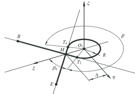
Fig. 2 shows the path of the end-effector’s movement with an implemented, local coordinate system ξηζ.
Fig. 2. Path of motion with the introduced local coordinate system
The acceleration profile on a straight BM section is described by a 7th degree polynomial being used only at the first part of the profile, which represents the start-up phase (a solid line in Fig. 1).In the initial point
Fig. 1). The maximum linear velocity on the BM and
ME segments is νmax. This velocity is also the end-effector velocity on the loop.
2.2 Calculations of Path Geometry
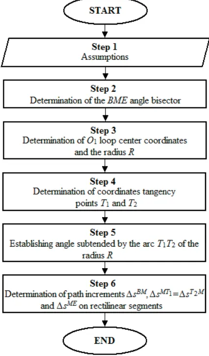
Flowchart in Fig. 3 presents the calculations of path geometry step by step.
Assume the following: the coordinates of the initial point B, the coordinates of the final point E, the coordinates of the point M, and distance from the point M to the center of a circle Δ. It is also possible
to assume the radius R, calculate the angle BME and
introduce into the algorithm the distance Δ calculated
using sine function of half angle BME.
Fig. 3. Flowchart for calculation of path geometry
Let a denote a vector of the start point B and end point M, while d is a vector starting at the point E and ending at the point M. Unit vectors of these vectors
will be a a a= / and d d d= / , respectively. The equation of the straight line on which the angle bisector
BME lies can be established using the coordinates of the point M and direction vector b, which is the sum of the unit vectors a and d.
Normalize vector b and the obtained unit vector
b multiplied by Δ value. The coordinates of the
vector calculated in this way should be added to the coordinates of the point M to obtain the coordinates of the O1 loop arc center. The radius R of a circle is determined as the distance from the center of the circle O1 to the line going through the points B and M (or the line going through the points E and M).
Calculate the distance between the tangency points and point M using the Pythagorean theorem. Multiply the calculated distance value by the unit vector a and add to the coordinates of the point M
to get the coordinates of the point T1, then multiply by the unit vector d and add to the coordinates of the point M to finally obtain the coordinates of point T2.
The angle β can be determined by adding to the angle π the angle between vectors a and d.
Path increments on the rectilinear segments are calculated using the coordinates of the starts and ends of the appropriate segments.
2.3 Calculations for the First Rectilinear Segment
For calculating the time of movement on the BM
section it is necessary to use a solution of a system of equations and use substitutions tf = 2tBM and
Δs = 2 ΔsBM. Finally:
t s
v
BM =105 BM
64 ∆
max
, (7)
where νmax is linear velocity in the motion through the
loop, which is simultaneously the maximum velocity on the rectilinear segment BM.
As for the motion along the MT1 segment, the following dependency should be utilized:
t s
v
MT1 MT
1
=∆
max
. (8)
The motion time on the BT1 segment is equal to the sum of tBM and tMT1 times.
The polynomial coefficient for the BM section can be calculated from the dependency:
p s
t
BM BM
BM
= ⋅
⋅ 315
8 9
∆
In order to determine the acceleration, velocity and dislocation profiles on the BM section, it is necessary to use dependencies (Eqs. (1) to (3)) and use substitutions tf = 2tBM and p = pBM.
2.4 Calculations for the arc
Motion time over the T1T2 arc is calculated from the formula:
t R
v
A= β⋅
max. (10)
The angular position for tBT1≤ ≤t tBT1+tA is
obtained from the following dependency considering the initial angular position βb:
β( )t β vmax ( ),
R t t
b BT
= + ⋅ − 1 (11)
where βb = −π ( / ).β 2
Coordinates of the position vector SA in the motion on the arc in the basic coordinate system
xyz are calculated using the transformation matrix T
between the local coordinate system ξηζ and basic system xyz:
SA= ⋅ΞT ΞA, (12)
where SA= s txA( ), s tyA( ), s tzA( ), 1T and
Ξ
ΞA=
[
R⋅cos ( ),β t R⋅sin ( ),β t 0 1,]
T.Velocities VA and accelerations AA are derived as the successive derivatives of the position vector SA.
2.4 Calculations for the Second Rectilinear Segment
The motion time on the T2M segment is the same as on the MT1 segment. In order to obtain motion time over the ME segment, the dependency (Eq. (7)) should
be used with the path increment ΔsME substitution. Motion time on the T2E segment is equal to the sum of
tT M2 and tME times. For the calculation of a polynomial
coefficient on a segment, use the Eq. (9) and substitute
path increment ΔsME and time tME in the formula. A
profile of acceleration, velocity, and position on the
ME segment can be derived in an analogous manner as with the BM segment, and each of them needs translation in the time by τ:
τ =tBT1+ +tA tT M2 −tME. (13)
2.5 Final Calculations
Motion time over the BT1T2E trajectory is calculated, summing up the motion times on the rectilinear segments and the motion time over the arc
te=tBT1+ +tA tT E2 . (14)
The linear path on the BT1T2E trajectory is calculated as the sum of the path on the rectilinear segments and the path over the arc.
3 NUMERICAL EXAMPLE
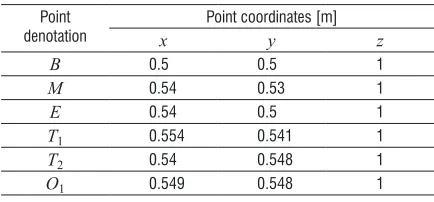
The coordinates of the points for the prescribed end-effector trajectory B, M, E, the center of loop O1 and tangent points T1, T2 are presented in Table 1.
Table 1. Coordinates of characteristic points of trajectory Point
denotation x Point coordinates [m]y z
B 0.5 0.5 1
M 0.54 0.53 1
E 0.54 0.5 1
T1 0.554 0.541 1
T2 0.54 0.548 1
O1 0.549 0.548 1
The assumed distance between the center of loop
O1 and point M was Δ = 0.02 m. A calculated radius arc circle was R = 8.944×10⁻³ m, while the angle
β = 4.069 rad. The path increments on the
rectilinear segments are as follows: ∆sBM = 0.05 m,
∆sMT1 =∆sT M2 = 0.0179 m and ∆sME = 0.03 m. There was an assumed maximum velocity on the rectilinear segments νmax = 0.25 m/s. The motion times over the rectilinear segments BM and MT1 are tBM = 0.328 s and tMT1= 0.072 s, respectively, whereas for the
coefficient of the polynomial profile of acceleration, the velocity and position for the segment BM was
pBM
232 =4 46156 10. × 4m/s9. The motion time through the loop arc tA = 0.146 s and the initial angle value was βp = 1.107 rad. The motion times on the rectilinear segments T2M and ME were as follows:
tT M2 =0.072 s and tME = 0.197 s, while the coefficient
of the polynomial profile of acceleration, velocity and position for the segment ME was pME = 2.65844×10⁶ m/s9. The translation in time was τ = 0.42 s, whereas the total motion time te = 0.815 s. The total path along
the motion trajectory was Δs = 0.152 m, while on the
loop ΔsA = 0.036 m.
Fig. 4. The assumed end-effector’s path in a coordinate system xyz
4 SIMULATION RESULTS
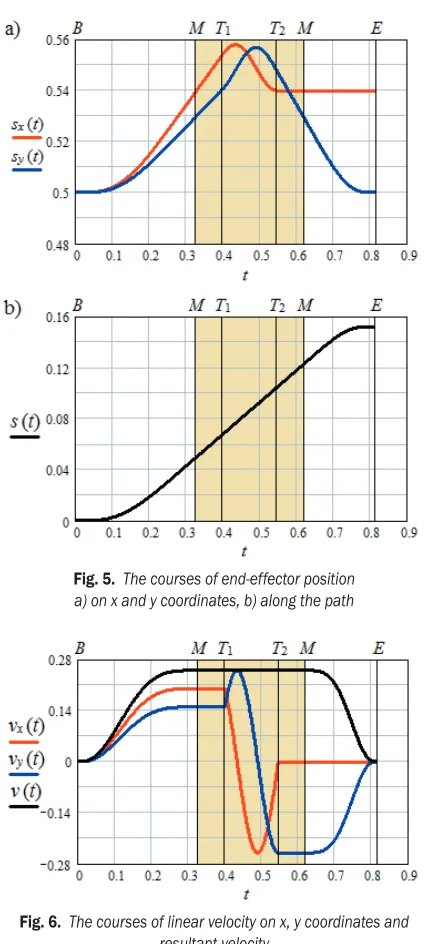
Fig. 5a gives the course of end-effector positions along the axes x and y, whereas Fig. 5b is the course of end-effector positions along the prescribed trajectory. Fig. 6 presents the courses of velocity components of the end-effector toward the axes x
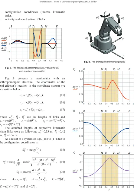
and y, and the run of the resultant velocity. During the motion through the loop (on the rectilinear segments MT1 and T2M and arc T1T2), the resultant velocity does not change and is equal to the preset one νmax = 0.25 m/s, while on the segments BM and ME it changes in accordance with the assumed profile. The components of velocity along axes x and y are obtained through the projection of the resultant velocity vector onto the directions of the coordinate system xyz. The changes in the components on the segments BM and ME are associated with changes in the resultant velocity, while the change in velocity components on the loop are associated with changes in the direction of a constant vector of resultant velocity. Both the runs of the components and the resultant velocity run are continuous functions considering the value. Fig. 7 presents the course of acceleration components in the x, y direction, and the course of resultant acceleration. A profile of resultant acceleration and acceleration components at points B,
M, E, are tangential to the time axis and their value is equal to zero. The acceleration value is also equal to zero on the segments MT1 and T2M. The jump in the acceleration value on the arc T1T2 results from the motion on curved path. Tangential acceleration in motion along an arc equals zero, while centripetal
acceleration is proportional to the square of the velocity and is inversely proportional to the radius of the arc. The changing direction of centripetal acceleration results in a change in components in the direction x and y. The period of movement on the
MT1T2M loop is marked in addition.
Fig. 5. The courses of end-effector position a) on x and y coordinates, b) along the path
Fig. 6. The courses of linear velocity on x, y coordinates and resultant velocity
The suggested method of trajectory planning is used to simulate a motion of three manipulators. For each of the manipulators, the following are determined:
• configuration coordinates (inverse kinematic task),
• velocity and acceleration of links.
Fig. 7. The courses of acceleration on x, y coordinates, and resultant acceleration
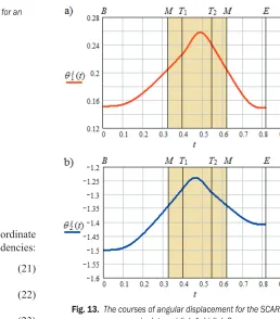
Fig. 8 presents a manipulator with an anthropomorphic structure. The coordinates of the end-effector’s location in the coordinate system xyz
are written below:
sx=c l c l c1 2 2(a + 3 23a ), (15)
sy=s l c l ca + a
1 2 2( 3 23), (16)
sz =λ1a+l s l s2 2a + 3 23a , (17)
where λ1a, l2a, l3a are the lengths of links and
ci =cos( )θia , si =sin( )θia , cij=cos(θia+θja),
sij ia
j a =sin(θ +θ ).
The assumed lengths of respective kinematic chain links were as following λ1a=0.33 m, l2a=0.42 m, l3a=0.36 m.
As a result of a system of Eqs. (15) to (17) due to the configuration coordinates is:
θ1a y
x
s s
=arctg( ), (18)
θ2a A 2 2 22 2
B
C B A D
E B A
= − − + −
+
arctg arcsin ( )
( ) , (19)
θ3a B A D2
C
=arccos( + − ), (20)
where A s= z−λ1a, B s= 2x+sy2, C=2l l2 3a a,
D=( )la +( )la
2 2 3 2 and E=2l2a.
Courses of links’ angular displacements for the generated trajectory are presented in Fig. 9.
Fig. 8. The anthropomorphic manipulator
The course of velocities and accelerations of links is presented on Figs. 10 and 11.
Fig. 10. The courses of angular velocity of links for an anthropomorphic manipulator
Fig. 11. The courses of angular acceleration of links for an anthropomorphic manipulator
Fig. 12 shows the SCARA manipulator.
Fig. 12. The SCARA manipulator
Coordinates of the end-effector in the coordinate
xyz system are defined by the following dependencies: sx=l c l cs + s
1 1 2 12, (21)
sy=l s l ss + s
1 1 2 12, (22)
sz=λ1s+λ2s−λ3s (23)
where λ1s, λ
2s, l1s, l2s are the lengths of the links, while ci=cos( )θis , si=sin( )θis , cij=cos(θis+θjs),
sij =sin(θis+θjs).
The assumed lengths of particular links of respective kinematic chain were as following
λ1s=0.3 m, λ2s=0.065 m, l1s=0.54 m, l2s=0.42 m. As a consequence of the equation system (Eqs. (21) to (23)), and due to configuration coordinates, the below was obtained:
θ1a y 2 2 2
x s s
C B D
E B
=arctg( )−arcsin( −( − ) ), (24)
θ2a B D
C
= −arccos( − ), (25)
λ3s λ1s λ2s z s
= + − , (26)
where B s= x2+sy2, C=2l l1 2s s, E=2l1s and D=( )ls +( )ls
1 2 2 2.
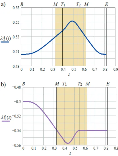
The courses of angular accelerations in the kinematic pairs of the SCARA manipulator for a planned trajectory are presented in Fig. 13 (coordinate
λ3s was skipped because it has a constant value). The velocities and link angular accelerations are presented in Figs. 14 and 15.
Fig. 14. The courses of angular velocity for the SCARA manipulator
Fig. 15. The courses of angular acceleration for the SCARA manipulator
Fig. 16 shows a manipulator with a Cartesian structure.
Fig. 16. The Cartesian manipulator
The coordinates of end-effector position in the
xyz coordinate system are:
sx= −λ3c, (27)
sy=λc
2, (28)
sz=λ1c+l2c, (29)
where lc
2 is the length of manipulator’s link and lc
2 =0.24m.
As a result of the equation system solution (Eqs. (27) to (29)), and due to configuration coordinates, the following is obtained:
λ1c 2
z c s l
= − , (30)
λ2c=sy, (31)
λ3c= −sx. (32)
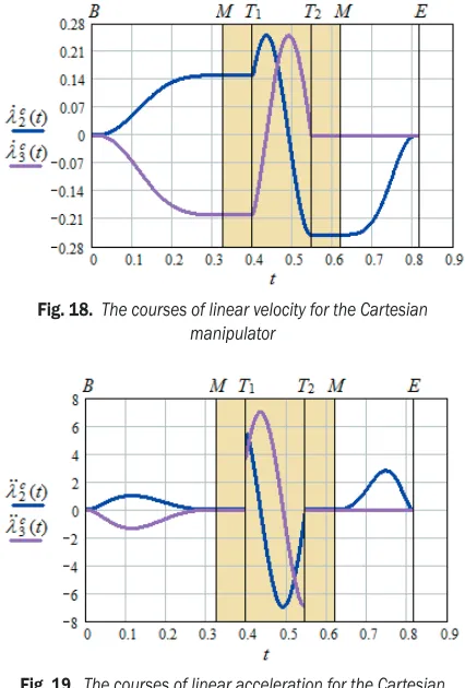
The courses of displacement of links for the kinematic chain studied for a planned trajectory are presented in Fig. 17 (λ1c coordinate was skipped because it has a constant value).
Fig. 17. The courses of linear displacement for the Cartesian manipulator a) link 2, b) link 3
Velocities and linear accelerations of the links are presented in Figs. 18 and 19.
Fig. 18. The courses of linear velocity for the Cartesian manipulator
Fig. 19. The courses of linear acceleration for the Cartesian manipulator
5 CONCLUSIONS
In order to obtain high accuracy mapping of a trajectory with concomitant full utilization of machine dynamic capabilities, it is necessary to generate smooth trajectories with minimum jerk constraints, acceleration or velocity. This paper proposes a method for planning a rectilinear-arc trajectory in which two opposite requirements meet, i.e. trajectory smoothing and simultaneous passing through a sharp corner. The simulation tests performed allowed for the formulation of the following final remarks:
1. For the reason that a tool passes through the point
M twice, the generated motion trajectory can be used both, as a whole – BT1T2E or in part – BME. In the latter case, the on-loop motion MT1T2M can be treated as the tool output.
2. At the characteristic points B, M, E of the trajectory, the acceleration profile is tangential to the time axis which causes zero jerk value at these points.
3. The algorithm is effective for calculations. The most laborious prove to be the calculations of trajectory geometry, whereas to obtain a profile of
position, velocity and acceleration, it is sufficient to calculate a polynomial coefficient and motion time.
4. The simulation results indicate the applicability of the proposed method in the analysis stage as well as the design of manipulators and machine tools.
Further studies will be needed to determine the effect of loop size on trajectory mapping accuracy, taking into account the deformability of manipulator kinematic chains.
6 REFERENCES
[1] Boryga, M., Graboś, A. (2009). Planning of manipulator
motion trajectory with higher-degree polynomials use.
Mechanism and Machine Theory, vol. 44, no. 7, p.
1400-1419, DOI:10.1016/j.mechmachtheory.2008.11.003. [2] Chettibi, T. (2006). Synthesis of dynamic motions
for robotic manipulators with geometric path constraints. Mechatronics, vol. 16, no. 9, p. 547-563, DOI:10.1016/j.mechatronics.2006.03.012.
[3] Constantinescu, D., Croft, E.A. (2000). Smooth and time-optimal trajectory planning for industrial manipulators along specified path. Journal of Robotic
Systems, vol. 17, no. 5, p. 233-249, DOI:10.1002/
( S I C I ) 1 0 9 7 4 5 6 3 ( 2 0 0 0 0 5 ) 1 7 : 5 < 2 3 3 : : A I D -ROB1>3.0.CO;2-Y.
[4] Elnagar, A., Hussein, A. (2000). On optimal constrained trajectory planning in 3D environments. Robotics
and Autonomous Systems, vol. 33, no. 4, p. 195-206,
DOI:10.1016/S0921-8890(00)00095-6.
[5] Gasparetto, A., Zanotto, V. (2007). A new method for smooth trajectory planning of robot manipulators.
Mechanism and Machine Theory, vol. 42, no. 4, p.
455-471, DOI:10.1016/j.mechmachtheory.2006.04.002. [6] Gasparetto, A., Zanotto, V. (2008). A technique for
time-jerk optimal planning of robot trajectories.
Robotics and Computer-Integrated Manufacturing, vol.
24, no. 3, p. 415-426, DOI:10.1016/j.rcim.2007.04.001. [7] Machmudah, A., Parman, S., Zainuddin, A., Chacko,
S. (2012). Polynomial joint angle arm robot motion planning in complex geometrical obstacles. Applied
Soft Computing, vol. 13, no. 2, p. 1099-1109,
DOI:10.1016/j.asoc.2012.09.025.
[8] Perumaal, S., Jawahar, N. (2012). Synchronized trigonometric S-curve trajectory for jerk-bounded time-optimal pick and place operation. International Journal of Robotics & Automation, vol. 27, no. 4, p. 385-395, DOI:10.2316/Journal.206.2012.4.206-3780.
[9] Tian, L.F., Collins, C. (2003). Motion planning for redundant manipulators using a floating point genetic algorithm. Journal of Intelligent & Robotic
Systems, vol. 38, no. 3-4, p. 297-312, DOI:10.1023/
B:JINT.0000004973.29102.33.
Chinese Journal of Mechanical Engineering, vol. 23, no. 2, p. 135-141, DOI:10.3901/CJME.2010.02.135. [11] Chen, Y., Wei, H., Sun, K., Liu, M., Wang, T.
(2011). Algorithm for smooth S-curve feedrate profiling generation. Chinese Journal of Mechanical
Engineering, vol. 24, no. 2, p. 237-247, DOI: 10.3901/
CJME.2011.02.237.
[12] Du, D., Liu, Y., Guo, X., Yamazaki, K., Fujishima, M. (2010). An accurate adaptive NURBS curve interpolator with real-time flexible acceleration/ deceleration control. Robotics and
Computer-Integrated Manufacturing, vol. 26, no. 4, p. 273-281,
DOI:10.1016/j.rcim.2009.09.001.
[13] Emami, M.M., Arezoo, B. (2010). A look-ahead command generator with control over trajectory and chord error for NURBS curve with unknown arc length. Computer-Aided Design, vol. 42, no. 7, p. 625-632, DOI:10.1016/j.cad.2010.04.001.
[14] Erkorkmaz, K., Altintas, Y. (2001). High speed CNC system design. Part I: jerk limited trajectory generation and quintic spline interpolation. International Journal
of Machine Tools & Manufacture, vol. 41, no. 9, p.
1323-1345, DOI:10.1016/S0890-6955(01)00002-5. [15] Farouki, R.T., Tsai, Y.F., Wilson, C.S. (2000). Physical
constraints on feedrates and feed accelerations along curved tool paths. Computer Aided Geometric Design, vol. 17, no. 4, p. 337-359, DOI:10.1016/S0167-8396(00)00004-2.
[16] Nam, S.H., Yang, M.Y. (2004). A study on a generalized parametric interpolator with real-time jerk-limited acceleration. Computer-Aided Design, vol. 36, no. 1, p. 27-36, DOI:10.1016/S0010-4485(03)00066-6.
[17] Stori, J.A., Wright, P.K. (2000). Constant engagement tool path generation for convex geometries. Journal
of Manufacturing Systems, vol. 19, no. 3, p. 172-184,
DOI:10.1016/S0278-6125(00)80010-2.
[18] Zheng, C., Su, Y., Mueller, P.C. (2009). Simple online smooth trajectory generations for industrial systems. Mechatronics, vol. 19, no. 4, p. 571-576, DOI:10.1016/j.mechatronics.2008.11.017.
[19] Kovacic, M., Balic, J. (2003). Evolutionary programming of a CNC cutting machine. International
Journal of Advanced Manufacturing Technology, vol.
22, no.1-2, p. 118-124, DOI:10.1007/s00170-002-1450-8.
[20] Lloyd, J., Hayward, V. (1993). Trajectory generation for sensor-driven and time-varying tasks. International
Journal of Robotics Research, vol. 12, no. 4, p.
380-393, DOI:10.1177/027836499301200405.
[21] Macfarlane, S., Croft, E.A. (2003). Jerk-bounded manipulator trajectory planning: design for real-time applications. IEEE Transactions on Robotics and
Automation, vol. 19, no. 1, p. 42-52, DOI:10.1109/
TRA.2002.807548.
[22] Erkorkmaz, K., Yeung, C.H., Altintas, Y. (2006). Virtual CNC system. Part II. High speed contouring application. International Journal of Machine Tools
& Manufacture, vol. 46, no. 10, p. 1124-1138,
DOI:10.1016/j.ijmachtools.2005.08.001.
[23] Dong, J., Ferreira, P.M., Stori, J.A. (2007). Feed-rate optimization with jerk constraints for generating minimum-time trajectories. International Journal of Machine Tools & Manufacture, vol. 47, no. 12-13, p. 1941-1955, DOI:10.1016/j.ijmachtools.2007.03.006. [24] Tsai, M.S., Nien, H.W, Yau, H.T. (2008). Development
of an integrated look-ahead dynamics-based NURBS interpolator for high precision machinery. Computer-Aided Design, vol. 40, no. 5, p. 554-566, DOI:10.1016/j. cad.2008.01.015.
[25] Tseng, S.J., Lin, K.Y., Lai, J.Y., Ueng, W.D. (2009). Nurbs curve interpolator with jerk-limited trajectory planning. Journal of the Chinese Institute of Engineers, vol. 32, no. 2, p. 215-228, DOI:10.1080/02533839.200 9.9671498.
[26] Wang, X., Wang, J., Rao, Z. (2010). An adaptive parametric interpolator for trajectory planning.
Advances in Engineering Software, vol. 41, no. 2, p.
180-187, DOI:10.1016/j.advengsoft.2009.09.010. [27] Grabos, A., Boryga, M. (2013). Trajectory planning of
end-effector with intermediate point. (Eksploatacja i
Niezawodnosc) Maintenance and Reliability, vol. 15,