Vol 4, No. 1, (2014), pp 77-94
An approximation method for
numerical solution of
multi-dimensional feedback delay
fractional optimal control problems by
Bernstein polynomials
E. Safaie∗ and M. H. Farahi
Abstract
In this paper, we present a new method for solving fractional optimal control problems with delays in state and control. This method is based upon Bernstein polynomials basis and feedback control. The main advantage of feedback or closed-loop control is that one can monitor the effect of such control on the system and modify the output accordingly. In this work, we use Bernstein polynomials to transform the fractional time-varying multi-dimensional optimal control system with both state and control delays, into an algabric system in terms of the Bernstein coefficients approximating state and control functions. We use Caputo derivative of degree 0< α≤1 as the fractional derivative in our work. Finally, some numerical examples are given to illustrate the effectiveness of this method.
Keywords: Delay fractional optimal control problem; Caputo fractional derivative; Bernstein polynomial.
1 Introduction
The general definition of an optimal control problem requires the minimiza-tion of a funcminimiza-tional over an admissible set of control and state funcminimiza-tions
sub-∗Corresponding authour
Received 25 November 2013; revised 29 January 2014; accepted 5 March 2014 E. Safaie
Department of Applied Mathematics, Faculty of Mathematical Sciences, Ferdowsi univer-sity of Mashhad, Mashhad, Iran. e-mail: [email protected]
M. H. Farahi
Department of Applied Mathematics, Faculty of Mathematical Sciences, Ferdowsi univer-sity of Mashhad, Mashhad, Iran,
and
The center of Excellence on Modelling and Control Systems (CEMCS), Mashhad, Iran. e-mail: [email protected]
ject to dynamic constraints on the states and controls. A Fractional Optimal Control Problem (FOCP) is an optimal control problem in which either the performance index or the differential equations governing the dynamic of the system or both contain at least one fractional order derivative term [1, 2, 17].
Fractional Differential Equations ( FDEs ) have been the focus of many studies due to their appearance in various applications in real-world physical systems. For example, it has been illustrated that materials with memory and hereditary effects and dynamical processes including gas diffusion and heat conduction can be more adequately modeled by FDEs than integer-order differential equations [13, 18, 20]. Some other applications of FDEs are in behaviors of viscoelastic materials, biomechanics and electrochemical processes ( see [3, 5] for more details ).
Most FOCPs do not have exact solutions, so in these cases approximation methods and numerical techniques must be used. Recently, several approxi-mation methods to solve FOCPs have been introduced [4, 14, 18].
Real life phenomena have been described more precisely by Delay Differ-ential Equations, so Delay Fractional Optimal Control Problem ( DFOCP ) has become the focus of many researchers in the last decade. Baleanu in [6] and Jarad in [11] analyzed the fractional variational principles for some kinds of DFOCPs within Riemann-Liouville and Caputo fractional derivatives re-spectively and made their corresponding Euler-Lagrange equations. In this paper, we present a novel strategy based on Bernstein polynomials (BPs) to solve DFOCPs. Consider the following DFOCP
M in J =1 2
∫1 0[x
T(t)Q(t)x(t) +uT(t)R(t)u(t)]dt, (1)
s.t
c 0D
α
txi(t) = Σ r
j=1ai,j(t)xj(t) + Σ s
k=1bi,k(t)uk(t) +Σr
j=1(ad)i,j(t)xj(t−η1) + Σsk=1(bd)i,k(t)uk(t−η2), 1≤i≤r, (2)
xj(t) =xj,0, t∈[−η1,0], 1≤j≤r,
uk(t) =uk,0, t∈[−η2,0], 1≤k≤s,
(3)
where x(t) = [x1(t)· · ·xr(t)]T and u(t) = [u1(t)· · ·us(t)]T are respectively the state and control functions. Also, Q(t) andR(t) are respectively, r×r
and s×s semi-positive and positive definite time-varying matrices of the state and control’s coefficients in the cost function with continuous functions as their entries. Furthermore, ai,j(t), (ad)i,j(t), bi,k(t) and (bd)i,k(t) are continuous functions which are respectively the coefficients of xj(t), xj(t− η1) for (1 ≤ j ≤ r) and uk(t), uk(t −η2) for (1 ≤ k ≤ s) in the i-th fractional differential equation (2) andη1, η2>0 are given constant delays. The fractional derivative is defined in Caputo sense, i.e.
c 0D
α txi(t) =
{ 1 Γ(1−α)
∫t 0(t−τ)
−α d
dτxi(τ)dτ,0< α <1, ˙
xi, α= 1.
In the numerical solution of dynamical systems, polynomials or piecewise polynomial functions are often used to present the approximate solutions [9, 10, 21]. The effectiveness of using Bernstein polynomials for solving FOCPs have been demonstrated before [4, 14]. In the present paper, we seek an optimal feedback control function to find the approximate solution of DFOCP (1) - (3) by using Bernstein polynomials.
This paper is organized as follows. In Section 2 we give some preliminiaries in fractional calculus. In Section 3 Bernstein polynomials are introduced and their properties are shown in several lemmas. In Section 4, a FOCP with time delay will be solved using BPs. Section 5 contains some numerical examples. Finally Section 6 consists of a brief conclusion.
2 Some preliminaries in fractional calculus
Definition 2.1. A real functionf(t), t >0, is said to be in the spaceCµ,
µ ∈ R, if there exists a real number p > µ such that f(t) = tpf
1(t), where
f1(t) ∈ C[0,+∞) and it is said to be in the space Cµm iff f(m) ∈ Cµ for
m∈N.
Definition 2.2. The Riemann-Liouville fractional integral operator of order
α >0of a function f ∈Cµ,µ >1, is defined as:
0Itαf(t) =Γ(1α) ∫t
0(t−τ) α−1
f(τ)dτ,
0It0f(t) =f(t).
(5)
Definition 2.3. The fractional derivative of f(t) in the Caputo sense is defined as follows:
c 0D
α tf(t) =
1 Γ(1−α)
∫ t
0
(t−τ)−α d n
dτnf(τ), n−1< α < n, n∈N, f∈C m
−1. (6) In [15], the following properties forf ∈Cµ andµ≥ −1 have been proved
1. 0Itαtk=
Γ(k+1) Γ(k+1+α)t
α+k, k∈N∪ {0}, t >0,
2. c0Dαt0Itαf(t) =f(t),
3. 0Itαc0Dtαf(t) =f(t)− ∑n−1
k=0f(0 +)tk
k!, t >0,
4. c 0D
β
3 Properties of Bernstein polynomials
The Bernstein polynomial of degree n over the interval [a, b] is defined as follows:
Bi,n (
t−a b−a
) = ( n i )(
t−a b−a
)i(
b−t b−a
)n−i
,
so, within the interval [0,1] we have
Bi,n(t) = (
n i
)
ti(1−t)n−i.
Define Φm(t) = [B0,m(t)B1,m(t) · · · Bm,m(t)]T. To consider the vector Φm(t−η) ( η is the given delay ) in terms of Φm(t), we state the follow-ing lemmas.
Lemma 3.1. We can write Φm(t) = ΛTm(t), where Λ = (Υi,j)mi,j+1=1 is an upper triangular(m+ 1)×(m+ 1) matrix with entry
Υi+1,j+1= {
(−1)j−i(mi)(mj−−ii), i≤j,
0, i > j, i, j= 0,1,· · · , m,
andTm(t) = [1t · · · tm]T.
Proof. [4].
Lemma 3.2. For each given constant delay η >0, Φm(t−η) = ΩΦm(t), whereΩis an (m+ 1)×(m+ 1)matrix in terms of η.
Proof. According to Lemma 3.1 we have
Φm(t−η) = ΛTm(t−η).
But, the right hand side of the above equation can be written as
ΛTm(t−η) = Λ 1
t−η
(t−η)2 .. . (t−η)m
= ΛΨ 1 t t2 .. . tm
= ΛΨTm(t),
Ψ =
1 0 0 · · · 0
−η 1 0 · · · 0
η2 −2η 1 · · · 0
..
. ... . .. ...
(−η)m(mm−1)(−η)m−1 · · · 1 .
By Lemma 3.1,Tm(t) = Λ−1Φm(t), thus
Φ(t−η) = ΛΨΛ−1Φm(t) = ΩΦm(t). □ (7)
Lemma 3.3. Let L2[0,1] be a Hilbert space with inner product ⟨f, g⟩ = ∫1
0 f(t)g(t)dt and y ∈ L
2[0,1]. Then one can find the unique vector C = [c0 c1 · · · cm]T such that
y(t)≈ m ∑
i=0
ciBi,m(t) =CTΦm(t). (8)
Proof. [12].
In Lemma 3.3 we haveCT =Q−1⟨y,Φm⟩such that
⟨y,Φm⟩= ∫ 1
0
y(t)Φm(t)dx= [⟨y, B0,m⟩ ⟨y, B1,m⟩ · · · ⟨y, Bm,m⟩]T,
and each entry of the matrixQ= (Qi+1,j+1) m
i,j=0 is defined as follows:
Qi+1,j+1= ∫ 1
0
Bi,m(t)Bj,m(t)dx= (m
i )(m
j )
(2m+ 1)(i2+mj).
Since the set {B0,m(t), B1,m(t),· · ·, Bm,m(t)} forms a basis for the vector space of polynomials of real coefficients and degree no more than m[7, 16], a polynomial of degreemcan be expanded in terms of a linear combination ofBi,m(t),(i= 0,1,· · · , m) as follows
P(t) = m ∑
i=0
ciBi,m(t),
moreover we have
tk = m∑−1
i=k−1 (i
k ) (m
k
)Bi,m(t).
Lemma 3.4.Derivatives ofPn(f) = ∑n
j=0f( j
to corresponding derivatives of f. So iff ∈Ck[0,1]then
limn→∞(Pn(f))(k)=f(k),
uniformly on [0, 1].
Proof. [8].
4 Fractional optimal control problem with delays in
control and state
Consider fractional delay control system (2). For each 0 ≤i ≤r, one can apply the Riemann-Liouville fractional integral 0Itα to both sides of that equation
xi(t)−xi(0) = Σr
j=10Itα{ai,j(t)xj(t)}+ Σks=10Itα{bi,k(t)uk(t)}+ Σr
j=10Itα{(ad)i,j(t)xj(t−η1)}+ Σsk=10I α
t{(bd)i,k(t)uk(t−η2)}. (9)
Assume thatxi(t)≈XT
i Φm(t) (1≤i≤r) anduk(t)≈UkTΦm(t) (1≤k≤s) where the entries Xi = [Xi(0)· · ·Xi(m)]T and Uk = [Uk(0)· · ·Uk(m)]T are respectively the coeffitients ofxi(t) anduk(t) in approximating them by Bern-stein polynomials of degree m just like (8). Moreover, the BernBern-stein approxi-mated coefficients vectors of functionsai,j(t),bi,k(t), (ad)i,j(t) and (bd)i,k(t) can be achieved by using equation (8). We denote the approximated vector coefficients of these functions respectively by (Ai,j)(m+1)×1, (Bi,k)(m+1)×1, (Ai,jd )(m+1)×1 and (B
i,k
d )(m+1)×1.
By substituting the so called approximated vectors and matrices in (1), one can find the following equations:
XiTΦm(t)−xi,0= Σrj=10I α
t{((Ai,j)TΦm(t))(XjTΦm(t)) T} +Σs
k=10I α
t{((Bi,k)TΦm(t))(UkTΦm(t))T} +Σrj=10Itα{((Ai,jd )TΦm(t))(XjTΦm(t−η1))T} +Σs
k=10Itα{((B i,k d )
TΦm(t))(UT
kΦm(t−η2))T}.
(10)
Moreover, from Lemma 3.2 there exist (m+ 1)×(m+ 1) matrices Ω1,Ω2 where Φm(t−η1) = Ω1Φm(t) and Φm(t−η2) = Ω2Φm(t), while
Ω1= ΛΨΛ−1,
Ω2= ΛΨ
′
Λ−1,
and Ψ,Ψ′ are obtained respectively in terms ofη1 andη2.
matricesA˜i,j,B˜i,k,A˜i,j
d and
˜
Bdi,k can be calculated such that:
(Ai,j)TΦm(t)ΦTm(t) = Φ T m(t) ˜Ai,j, (Bi,k)TΦm(t)ΦTm(t) = Φ
T
m(t) ˜Bi,k, (Ai,jd )TΦm(t)ΦTm(t) = Φ
T m(t)
˜
Ai,jd ,
(Bi,kd )TΦm(t)ΦTm(t) = Φ T m(t)
˜
Bdi,k.
Therefore, by replacing the above equalities, (2) can be rewritten as follows:
XiTΦm(t)−xi,0= Σrj=1(0ItαΦ T
m(t))( ˜Ai,jXj) + Σ s
k=1(0ItαΦ T
m(t))( ˜Bi,kUk)+ Σr
j=1(0ItαΦTm(t))( ˜
Ai,jd ΩT
1Xj) + Σsk=1(0ItαΦTm(t))( ˜
Bdi,jΩT 2Uk), or
XiTΦm(t)−xi,0= Σrj=1( ˜Ai,jXj)T(0ItαΦm(t)) + Σ s
k=1( ˜Bi,kUk)T(0ItαΦm(t))+ Σr
j=1( ˜
Ai,jd ΩT
1Xj)T(0ItαΦm(t)) + Σsk=1( ˜
Bdi,jΩT
2Uk)T(0ItαΦm(t)). (11) wherei= 1,· · ·, r.
One can approximate0ItαΦm(t) byIα×Φm(t), whereIαis an (m+ 1)× (m+ 1) matrix called the operational matrix of Riemann-Liouville fractional integral.
Infact, from Lemma 3.1, Φm(t) = ΛTm(t), so
0ItαΦm(t) = Λ 0ItαTm(t) = Λ [0Itα1 0Itαt · · · 0Itαt m]T,
where0Itαt
j= Γ(j+1) Γ(j+1+α)t
j+α. Therefore,
0ItαTm(t) = ˜Σ ˜T , (12)
where ˜Σ = ( ˜Σi+1,j+1) and ˜T = ( ˜Ti+1) are respectively (m+ 1)×(m+ 1) and (m+ 1)×1 matrices, which are defined as follows:
˜
Σi+1,j+1= {
Γ(j+1)
Γ(j+1+α), i=j,
0, o.w, i, j= 0,· · ·, m
and
( ˜T)i+1=ti+α, i= 0,· · · , m.
Also, from Lemma 3.3, sinceti+α∈L2([0,1]) for each integeri(0≤i≤m), one can find the (m+ 1)×1 vector Pi such that
where Pi = Q−1⟨ti+α,Φm(t)⟩ and the entries of ¯Pi = ⟨ti+α,Φm(t)⟩ = [ ¯Pi,0P¯i,1 · · · P¯i,m]T can be attained as
¯
Pi,j= ∫ 1
0
ti+αBj,m(t)dt=
m!Γ(i+j+α+ 1)
j!Γ(i+m+α+ 2), i, j= 0,· · · , m.
Now ifP is an (m+ 1)×(m+ 1) matrix of the form [P0P1· · ·Pm], then from (12) and (13) we have
0ItαΦm(t)≈Λ ˜ΣP
TΦm(t), (14)
therefore,Iα= Λ ˜ΣPT is the aforementioned operational matrix of Riemann-Liouville fractional integral0Itα.
Hence, by replacing0ItαΦm(t) from (14) into (4) and writingxi,0in terms of BPs of degreem, equation (4) can be written as the following
XT
i Φm(t)−Xi,T0Φm(t) = Σrj=1( ˜Ai,jXj)T IαΦm(t) + Σsk=1( ˜Bi,kUk)T IαΦm(t) +Σrj=1(A˜i,jd ΩT1Xj)T IαΦm(t) + Σsk=1(
˜
Bi,jd ΩT2Uk)T IαΦm(t), (15) where
Xi,T0= [Xi,0(0),· · ·, Xi,0(m)]T
is the known Bernstein approximated coefficents vector of xi,0 that can be computed using (8). By equalling the coefficents of Φm(t) from both sides of (5), we found that
XT
i =Xi,T0+ Σrj=1XjT( ˜Ai,j)T Iα+ Σsk=1U T k( ˜Bi,k)
T I α +Σr
j=1XjTΩ1(A˜i,jd )T Iα+ Σsk=1UkTΩ2(B˜i,jd )T Iα,
(16) fori= 1,· · · , r. Equations (8) can be written in compact form as follows:
XT = Π +UTΓ, (17)
where Π and Γ are respectively 1×(m+ 1) and (m+ 1)×(m+ 1) matrices that can be obtained by the following
Π =X0T(Im+1−( ˜A+ ˜Ad)Iα)−1,
and
Γ = ( ˜B+ ˜Bd)Iα(Im+1−( ˜A+ ˜Ad)Iα)−1, andIm+1 is the (m+ 1)×(m+ 1) identity matrix.
Moreover, by applying the approximations x(t) ≈ (XT)1×r(m+1)Φm(t) and u(t) ≈ (UT)1×s(m+1)Φm(t) where XT = [X1T,· · ·, X
T
r] and U
T =
J =12∫01{xT(t)Q(t)x(t) +uT(t)R(t)u(t)}dt
≈ 1
2 ∫1
0{X
TΦm(t)(QTΦm(t)ΦT
m(t)X)T +UTΦm(t)(RTΦm(t)ΦTm(t)U)T}dt, (18) where Q = [Qi,j] and R = [Ri,j] that Qi,j, Ri,j are the (m+ 1)×1 vec-tors of Bernstein coefficents in approximatingQi,j(t) andRi,j(t) respectively. Therefore,
J ≈ 1
2 ∫ 1
0
{XTΦm(t)(ΦTm(t) ˜QX)T +UTΦm(t)(ΦTm(t) ˜RU)T}dt,
or
J ≈ 1
2 ∫ 1
0
{(XTΦm(t))(XTQ˜TΦm(t)) + (UTΦm(t))(UTR˜TΦm(t))}dt, (19)
where ˜Q= [ ˜Qi,j] and ˜R = [ ˜Ri,j]. AlsoQ˜i,j andR˜i,j are (m+ 1)×(m+ 1) matrices that can be calculated from
(Qi,j)TΦm(t)ΦTm(t) = ΦTm(t) ˜Qi,j,
(Ri,j)TΦm(t)ΦTm(t) = Φ T
m(t) ˜Ri,j. Let Zi,j = H
⊗ ˜
Qi,j and Wi,j = H
⊗˜
Ri,j, where ⊗
is the Kronecker product andH = [Hi,j](m+1)×(m+1) and each entryHi,j is defined by
Hi,j= ∫ 1
0
Bi,m(t)Bj,m(t)dt,
then (19) can be rewritten in compact form as:
J ≈1
2{(X
TZX) + (UTW U)}, (20)
whereZ = [zi,j] andW = [wi,j].
From (17) we know thatXT = Π +UTΓ, so the necessary condition that U minimizes (20) and satisfy (17) is that
∂J ∂U =X
T
ZΓT +UTW = 0,
so
U∗T =XTZΓTW−1. (21) The above equation gives the optimal feedback control and by replacing (21) in (17), we can easily find the optimal state as well.
ΦTm(t) ˜Ri,j =RTi,jΦm(t)ΦTm(t)>0, t∈[0,1],
therefore ˜Ri,j and as the result Wi,j = H
⊗ ˜
Ri,j are positive definite and consequently invertible matrices.
5 Convergence of the method
In this section, we show the convergence of the presented method discussed in this article. First we prove the following lemma.
Lemma 5.1. Let XTΦm(t) = ∑m
j=0XjBj,m(t) be the Bernstein
poly-nomial of order m that approximates the function x(t) ∈ L2[0,1]. Then 0Itα(XTΦm(t)), tends to0Itαx(t)asm tends to infinity.
Proof. By Lemma 3.3 we have
limm→∞ m ∑
j=0
XjBj,m(t) =x(t). (22)
SinceBj,m(t) is a continuous function, we have
limm→∞ ∫ t
0 ∑m
j=0XjBj,m(τ)
(t−τ)1−α dτ =limm→∞ m ∑
j=0
Xj ∫ t
0
Bj,m(τ) (t−τ)1−αdτ.
By (22) and from Definition 2.2, we obtain ∫ t
0
x(τ)
(t−τ)1−αdτ = Γ(α)limm→∞ m ∑
j=0
Xj 0ItαBj,m(t),
or
0Itαx(t) =limm→∞ m ∑
j=0
Xj 0ItαBj,m(t) =limm→∞XT0ItαΦm(t). (23)
limn→∞PTΦn(t) =limn→∞
∑n
j=0Pj,0Bj,n(t) ∑n
j=0Pj,1Bj,n(t) ..
. ∑n
j=0Pj,mBj,n(t) = ˜T =
tα
t1+α
t2+α .. .
tm+α
,
therefore, limn→∞Λ ˜ΣPTΦn(t) = Λ ˜Σ limn→∞PTΦn(t) = Λ ˜Σ ˜T , or as ex-plained in (12) and (13)
limn→∞IαΦn(t) =0ItαΦm(t). (24)
From (23) and (24) we reach
0Itαx(t) =limm→∞XT limn→∞IαΦn(t). Givenn≥mwill complete the proof. □
Theorem 5.1. The approximated solutions x¯(t) = ¯XTΦm(t) and u¯(t) = ¯
UTΦm(t) in which ( ¯X,U¯) is achieved from (17) and (21), converge to the optimal solutions x∗(t) andu∗(t)as the degree of the Bernstein polynomials tend to infinity.
Proof. Suppose Wm is the set of all (UT, XT)Φm(·) where X, U ∈ Rm+1 and satisfy (17), also W is the set of all (u(·), x(·)) satisfy (2) and (3). Let ¯U be the optimal solution of (20) where obtained from (21) and ¯X be the solution of (17) obtained by replacing ¯U in eqation (17). Therefore ( ¯UT,X¯T)Φm(·) ∈ Wm. By the convergence property of Bernstein polyno-mials, for ( ¯UT,X¯T)Φm(·), there exists a unique pair of functions (¯u(·),x¯(·)) such that
( ¯UT,X¯T)Φm(·)−→(¯u(·),x¯(·)) as m→ ∞.
Now according to Lemma 5.1 it is clear that (¯u(·),x¯(·))∈W. Moreover as
m→ ∞, thenJ( ¯UTΦm,X¯TΦm)−→J¯where ¯J is the value of cost function (1) corresponding to the feasible solution (¯u(·),x¯(·)). Now, since
W1⊆ · · · ⊆Wm⊆Wm+1 ⊆ · · · ⊆W,
consequently
InfW1J1≥ · · · ≥InfWmJm≥InfWm+1Jm+1≥ · · · ≥InfWJ.
LetJm∗ =InfWmJm, soJm∗ =J( ¯UTΦm,X¯TΦm). Furthermore, the sequence {Jm}∗ is nonincreasing and bounded bellow which converges to a number
¯
J ≥ InfWJ. We want to show that ¯J = limm→∞Jm∗ = InfWJ. Given
ε >0, let (u(·), x(·)) be an element inW such that
by the definition of infimum, such (u(·), x(·))∈W exists.
Since J(u, x) is continuous, for this value of ε, there exists N(ε) so that if
m > N(ε),
|J(u, x)−J(UTΦm, XTΦm)|< ε, (26) Now ifm > N(ε), then using (25) and (26) gives
J(UTΦm, XTΦm)< J(u, x) +ε < InfWJ+ 2ε,
on the other hand
InfWJ ≤Jm∗ =InfWmJm≤J(U
TΦm, XTΦm),
so
InfWJ ≤Jm∗ < InfWJ+ 2ε, or
0≤Jm∗ −InfWJ <2ε, whereεis chosen arbitrary. Thus
¯
J =limm→∞Jm∗ =InfWJ. □
6 Numerical examples
In this section we give some numerical examples and apply the method presented in Section 4 for solving them. Our examples are solved using
M atlab2011aon an Intel Core i5-430M processor with 4 GB of DDR3 Mem-ory. These test problems demonstrate the validity and efficiency of this tech-nique.
Example 6.1. Consider the following delay fractional optimal control prob-lem in which 0< α≤1,
min J = 12∫01[x2(t) +12u2(t)]dt,
s.t c0Dtαx(t) =−x(t) +x(t−13) +u(t)−12u(t−23), 0≤t≤1,
x(t) = 1, −13≤t≤0,
u(t) = 0, −23≤t≤0.
For α = 1, this problem has been numerically solved by applying hybrid functions based on Legendre polynomials in [19] and the objective value
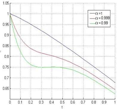
Figure 1: Approximate solution ofu(.) forα= 1,0.999,0.99 in Example 6.1
Table 1: The objective value and the end point of trajectory for α= 1,0.999,0.99 in Example 6.1
α objective value end-point
1 0.3956 0.6775
0.999 0.3283 0.6443
0.99 0.2907 0.6249
Table 2: The objective value and the end points of trajectories forα = 1,0.9,0.8 in Example 6.2
α objective value end points 1 0.7245 −0.4691, −0.0113 0.9 1.0291 −0.6477, 0.3202 0.8 0.7299 −0.4324, 0.4674
for some values ofαin Fig.1 and Fig.2. Moreover, for these values ofαthe objective values and the end points of optimal trajectory are shown in Table 1.
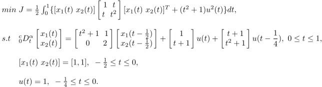
Example 6.2. Consider the following two-dimensional DFOCP in which 0< α≤1,
min J=1 2
∫1
0{[x1(t)x2(t)]
[ 1 t t t2
]
[x1(t)x2(t)]T+ (t2+ 1)u2(t)}dt,
s.t c0Dα t
[
x1(t)
x2(t) ]
= [
t2+ 1 1
0 2
] [
x1(t−12) x2(t−1
2)
] +
[ 1
t+ 1 ]
u(t) + [
t+ 1
t2+ 1
]
u(t−1
4), 0≤t≤1,
[x1(t)x2(t)] = [1,1], −1 2≤t≤0,
u(t) = 1, −14≤t≤0.
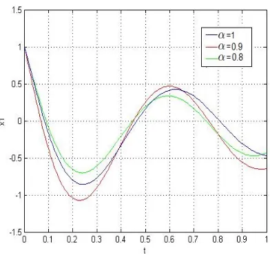
Figure 3: Approximate solution ofu(.) forα= 1,0.9,0.8 in Example 6.2
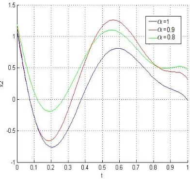
Figure 5: Approximate solution ofx2(.) forα= 1,0.9,0.8 in Example 6.2
7 Conclusion
In this paper, we peresent a new method of using Bernstein polynomials for solving DFOCP’s. We approximate the objective function and find a feed back control which minimizes the cost function. Then by replacing the optimal control in the constraints, we get an algabric system which can be solved in terms of the approximate coefficents of trajectory. The convergence of the method is extensively discussed and some test problems are included to show the efficiency of this very easy to use and accurate method.
References
1. Agrawal, O. P. A formulation and a numerical scheme for fractional optimal control problems, Journal of Vibration and Control, 14, (2008), 1291-1299.
2. Agrawal, O. P.A general formulation and solution scheme for fractional and optimal control problems, Nonlinear Dynamics, 38, (2004), 323-337.
4. Alipour, M., Rostamy, D. and Baleanu, D. Solving multi-dimensional fractional optimal control problems with inequality constraint by Bern-stein polynomials operational matrices, Journal of Vibration and Control, (2012), DOI:10.1177/1077546312458308.
5. Bagley, R. L. and Torvik, P. J.On the appearance of the fractional deriva-tive in the behavior of real materials, J. Appl. Mech., 51, (1984), 294-298.
6. Baleanu, D., Maaraba (Abdeljawad), T. and Jarad, F.Fractional varia-tional principles with delay, J. Phys. A: Math. Theor, 41, (2008), Article Number: 315403.
7. Farouki, R. and Rajan, V. On the numerical condition of polynomials in Bernstein form, Computer Aided Geometric Design, 4 (3), (1987), 191-216.
8. Floater, M. S. On the convergence of derivatives of Bernstein approxi-mation, Journal of Approximation Theory, 134, (2005), 130-135.
9. Ghomanjani, F., Farahi, M. H. and Gachpazan, M.Bezier control points method to solve constrianed quadratic optimal control of time varying linear systems, Computational and Applied Mathematics, 31, (2012), 34-42.
10. Ghomanjani, F. and Farahi, M. H.The Bezier control points method for solving delay diffrential equations, Intlligent Control and Automation, 3, (2012), 188-196.
11. Jarad, F, Abdeljawad (Maraaba), T. and Baleanu, D. Fractional varia-tional principles with delay within Caputo derivatives, Reports on Math-ematical Physics, 1, (2010), 17-28.
12. Kreyszig, E.Introduction to Functional Analysis with applications, John Wiley and Sons, New York, (1978).
13. Lopes, A. M., Tenreiro Machadob J. A, Pinto C. M. A. and Galhano A. M. S. F. Fractional dynamics and MDS visualization of earthquake phenomena, Computers and Mathematics with Applications, 66, (2013), 647-658.
14. Lotfi, A., Dehghan, M. and Yousefi, S. A. A numerical technique for solving fractional optimal control problems, Computers and Mathematics with Applications, 62, (2011), 1055-1067.
15. Oldham, K. B. and Spanier, J. The fractional calculus, New York: Aca-demic Press, (1974).
17. Tangprng, X. W. and Agrawal, O. P. Fractional optimal control of a continum system, ASME Journal of Vibration and Acoustic, 131, (2009), 232-245.
18. Tricaud, C. and Chen, Y. Q. An approximate method for numerically solving fractional order optimal control problems of general form, Com-puters and Mathematics with Applications, 59, (2010), 1644-1655.
19. Wang, X. T. Numerical solutions of optimal control for linear time-varying systems with delays via hybrid functions, Journal of the Franklin Institute, 344, (2007), 941-953.
20. Zamani, M., Karimi, G. and Sadati, N. FOPID controller design for robust performance using particle swarm optimization, J. Fract. Calc. Appl. Anal., 10, (2007), 169-188.