A New Parameter of Statistic Equality of Sampling Lengths in Surface Roughness Measurement

(1)

0 INTRODUCTION

Accelerated growth in the applications of surface metrology has led to significant changes in the approach to and study of surface metrology. However, the essence of surface metrology is that it must enable full control of surface constitution and provide an understanding of the characteristics that are important from a functional point of view.

In [1] and [2] there is a detailed and systemic description of the genesis of the surface metrology discipline, as well as the expected future development directions. The development of surface metrology, presented in [2], is shifting away from profile towards aerial characterization, away from stochastic towards structural surfaces, and away from simple shapes towards complex freeform geometries.

On the other hand, the current product surface roughness prediction models, at least for conventional machining, are based on a planar projection of the tool geometry (regardless of whether the geometry is defined or not) onto the surface of the work piece [3] and [4]. Hence the conclusion that studies of the roughness profile and the roughness parameters will continue to remain important, but that the emphasis will shift towards ways to determine them more accurately. This paper examines the conditions needed for a more accurate determination of the roughness profile and the roughness parameters by means of a new parameter: the statistical equality of sampling lengths.

1 PROCEDURE FOR OBTAINING THE ROUGHNESS PROFILE WHEN MEASURING SURFACE ROUGHNESS

The procedure for obtaining the roughness profile, and thereby the roughness parameters, has evolved together with improvements in measuring devices. In order to realiably compare the measured values of the roughness parameters, the procedures and recommendations used to measure and obtain the roughness profile are usually included in the national standards on a local level or in the international standards on global level, and these are usually harmonized with one another.

The paper provides an overview of the current ISO standards’ recommendations on obtaining roughness profiles using contact skidless instruments. This provides the procedure for obtaining the roughness profile illustrated in Fig. 1.

Before the measurement process is started, the section of the surface that will be measured should be determined. The reference system is placed so that the x-axis runs perpendicular to the process traces (the lay).

The intersection between the plane oriented along the x-axis and the surface irregularities determine the surface profile. The measurement can be made using any available measuring instrument that uses a stylus and a skidless probe. As the stylus traces the surface profile, the traced profile is determined by mechanical filtration, as shown in Position 4 in Fig. 1. The digitalized form of the traced profile facilitates the determination of the total profile, as shown in Position 5, which contains the nominal form, the roughness profile, and the waviness profile. The next step is to remove the nominal form from the total profile. If a flat surface is measured then, according to [5], the

A New Parameter of Statistic Equality of Sampling Lengths in

Surface Roughness Measurement

Tomov, M. – Kuzinovski, M. – Cichosz, P.

Mite Tomov1,*_{– Mikolaj Kuzinovski}1 _{– Piotr Cichosz}2

1 _{“Ss. Cyril and Methodius” University in Skopje, Faculty of Mechanical Engineering, Macedonia} 2 _{Wroclaw University of Technology, Institute of Production Engineering and Automation, Poland}

This paper presents the procedure for obtaining the primary profile, the waviness profile, and the roughness profile when measuring surface roughness, based on a set of recommendations from several ISO standards. An analysis was conducted and key insights into the procedure are given. In addition, a proposal to introduce a new parameter of statistical equality of sampling lengths when measuring surface roughness is included and the possible benefits from introducing the new parameter are stated.

(2)

µm 0 5 10 15 20

0 0.5 1 1.5 2 2.5 3 3.5 4 mm

Nominal form (removed)

IS O 32 74 :19 96 ISO 42 87 :1 99 7 6 µm -2 -1 0 1 2

0 0.5 1 1.5 2 2.5 3 3.5 mm

Application of the profil filter λs

IS O 4 28 7: 199 7; IS O 327 4: 199 6; IS O 11 56 2: 19 96 ; IS O 16 610 seri es … . Noise 7 -3.0 -2.0 -1.00.0 1.0 2.0 3.0

0 0.5 1 1.5 2 2.5 3 3.5 4

Waviness profile

Application of the profil filter λf

IS O 4 28 7: 19 97; IS O 32 74: 199 6; IS O 11 56 2: 19 96; IS O 16 61 0 s eri es … . 11 Traced profile IS O 3 27 4: 199 6 4 IS O 4 28 8: 199 6 IS O 3 27 4: 199 6 Measujhgvvhhhbrem ent process 3 Real surface Surface profile x z y IS O 42 87 :1 99 7 1 2 µm 0 1 2 3 4 5

0 0.5 1 1.5 2 2.5 3 3.5 4 mm

Total profile IS O 3 27 4: 199

6 5

µm

-2 -1 0 1

0 0.5 1 1.5 2 2 .5 3 3.5 4 m m

Primary profile IS O 3 27 4: 19

96 Mean line for the primary profile 8 -3 -2 -10 1 2 3

0 0.5 1 1.5 2 2.5 3 3.5 4

IS O 428 7: 199 7; IS O 3 27 4: 19 96 ; IS O 11 56 2: 19 96; IS O 16 61 0 s eri es … .

Application of the profil filter λc

9

Roughness paremeter Ra, Rq, Rt, Rp, Rv…..

12 µm -2 -1 0 1

0 0.5 1 1.5 2 2.5 3 3.5 mm

Mean line for the roughness profile IS O 4 28 7: 19 97 Roughness profile 10 Measurement process and ot he r.

Fig. 1. Procedure for obtaining the primary profile, the roughness profile, and the waviness profile

most frequently used method is the least squares mean line method (Position 6). The process of software filtering using the profile filters λs, λc and λf begins from Position 7 onwards and the application of the λs profile filter facilitates the removal of the elements with small amplitudes and large frequencies (for example: noise) from the total profile. The application

(3)

the primary profile, the mean line for the roughness profile is obtained, and the roughness profile (Position 10 in Fig. 1) is obtained when the values of the mean line coordinates are subtracted from the values of the primary profile coordinates. The roughness profile is described using R parameters (roughness parameters). When the components with long waveforms are removed from the mean line obtained by application of the λc profile filter, the waviness profile is obtained (Position 11 in Fig. 1). The waviness profile is described using W parameters.

2 THE NEED FOR INTRODUCING A NEW PARAMETER

The current definitions, mathematical formulations, and graphic interpretations of the parameters used to describe the primary profile and the roughness and waviness profiles are based on the M system, which requires the determination of the referent mean line in order to express and determine the parameters. The procedure presented in Fig. 1 clearly shows that the determination of the referent mean line for the purposes of determining the roughness profile is done through a filtering process using the λc profile filter. A great deal of research in the field of surface metrology is dedicated to studying the filtering as well as the metrological characteristics of the profile filters used.

The primary objective that the profile filters need to fulfill is to have the determined mean line pass through the center of the irregularities comprising the profile through which the mean line passes.

In practice, the most frequently used filter is the Gaussian filter. Its metrological characteristics for an open profile are standardized in [7] and [8].

Studies on the application of this profile filter have identified some disadvantages to its use [9] to [11]. Namely, the filter mean line determined using the Gaussian filter can be distorted at the ends of the profile as a result of the openness of the primary profile, which is not the case when applying the filter on closed profiles. Another disadvantage worth mentioning is its sensitivity to the deep grooves of the primary profiles, which leads to a false characterisation of the roughness profile in close proximity to the groove. An attempt has been made to remedy these disadvantages of the Gaussian profile filter with the introduction of ISO 13565-1:1996 [12], ISO 16610-21:2011 [13], and ISO/TS 16610-28:2010 [14]. ISO 13565-1:1996 proposes a special filtering method using the Gaussian filter on primary profiles with deep grooves, ISO 16610-21:2011 introduces several types of new Gaussian filters, and ISO/TS 16610-28:2010 presents a method for removing the possible

distortions at the end of the filter mean line. However, [9] and [10] emphasize that these deficiencies appear only when the primary profile is highly wavy, i.e. when the profile features sudden changes in the forms of the irregularities along its length.

Additional momentum in the research activities related to filtration in surface metrology has been provided by the International Standardization Organization (ISO) which, according to [1], issued a document (а resolution) designated as ISO/TC 213 in 1996 and established a working group. The primary aim of this group is filtration research. The initiative to form such a group came from the needs of the industry as well as from the frequent debates about the disadvantages of the most frequently used filters at the time, i.e. the Gaussian and the 2RC filter. The results of the work of this group have facilitated the establishment of a filter development framework (including the standards and technical specifications that will be developed in the future), but on a solely mathematical basis. The documents derived from the work of the working group are presented as technical specifications (ISO/TS 16610 series). The new profile filters currently introduced by the

ISO/TS 16610 series include: Gaussian filters [13],

Gaussian regression filters [15], Spline filters [16] and [17], Spline wavelets [18], Disk and horizontal line-segment filters [19], Scale space techniques [20], and Motif filters (under development).

During a real measuring process, the operator (the metrologist), shown in Position 9 in Fig. 1, faces a situation where he/she has to select an appropriate

λc profile filter with metrological characteristics

depending on the characteristics and the shape of the primary profile. However, the operator assesses the state (shape and character) of the primary profile qualitatively (high level of waviness, low level of waviness, significant or insignificant end distortions, etc.). This qualitative assessment of the primary profile is based on the experience and the conviction of the operator and can lead to an inappropriate selection of a profile filter type.

The in-depth analysis regarding the filtering process and the use of profile filters suggests that if the irregularities that comprise the total profile are evenly and uniformly accumulated around the mean line used to determine the primary profile, then the probability of drawing mean lines using any existing λc profile filter that will not fulfill the requirement to pass through the middle is minimal.

(4)

provide information about the irregularities in the total or the primary profile around the mean line.

Therefore, the introduction of the new parameter will help link the state of the profiles obtained from the topography with the methodology for obtaining the parameter values, as shown in Fig. 1, irrespective of whether they are parameters of the primary, waviness or the roughness profile, with an ultimate view to determining these parameters as accurately as possible.

3 A NEW PARAMETER FOR THE STATISTICAL EQUALITY OF SAMPLING LENGTHS

Our proposal is to have the new parameter determined after the drawing of the mean line for determining the primary profile, position 8 of Fig. 1, and the information that it should provide about the shape (state) of the profile should take into account the accumulation of the statistical characteristics around one value (the mean value).

If the surveyed profile obtained from the surface is considered as a set of points in a reference system, it is clear that the magnitudes that have to be included in the determination of the new parameters are the basic

distribution measures, i.e. mean arithmetic value, variation (dispersion), and the standard deviation.

To determine whether a function is stationary and ergodic or not, the mean value (statistical and temporal) for a given part of the function (of an exact size) should be compared to other parts of the function of the same size [21]. Henceforth, any further research will make use only of the methodology for comparing parts of the function, regardless of whether the profile is a stationary and an ergodic function. If this methodology is applied to the primary profile represented by discrete values in a reference system, then the statistical characteristics of the irregularities of a segment of the profile need to be compared to other segments of irregularities along the profile.

The segments (parts) whose basic statistical characteristics will be compared to each other are considered to be equal to the sampling length lr. This

value has already been standardized in [5]. This allows a direct connection to the software filtration, where the profile filter size is equal to the sampling length.

For the purposes of deriving the mathematical formulation of the new parameter, we will consider two theoretical cases of scattering the irregularities around the mean line.

Primary profile

x

z _{Approximately equal}

standard deviations Mean value of

primary profile

Standard deviation of primary profile

Different mean value

Sampling length

x

z

Mean value of primary profile

Approximately equal mean value

Different standard deviations

Primary profile

Sampling length

(5)

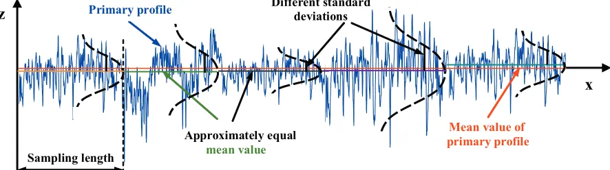
Case one: The points used to represent the primary profile within the sampling lengths have different mean values and approximately equal standard deviations, as shown in Fig. 2.

Case two: The points used to represent the

primary profile within the sampling lengths have approximately equal mean values and different standard deviations, as shown in Fig. 3.

The primary profiles in Figs. 2 and 3 are presented on a Cartesian right-oriented reference system, where the horizontal longitudinal axis is marked with x, while the vertical axis is the z-axis. The points used to represent the primary profile with its evaluation length and the sampling lengths, as parts of the primary profile, are considered to be the sample, since they are a part (sample) of the points that can be used to represent the entire surface topography. The points used to represent the entire surface topography are considered to be the population. Hence, the standard deviation for n data points is s, while the mean value for n data points z.

For the graphical presentation of the deviations sizes in Figs. 2 and 3, we have adopted the normal (Gaussian) distribution, although it is possible to have an abnormal distribution of irregularities within the sampling lengths.

In the first case,as a result of the scattering of the mean values of the sampling lengths around the mean line (mean value) of the primary profile, the standard deviation determined for the primary profile will be greater than the standard deviations of the individual sampling lengths. It can be observed that the lower the scatter of the mean values of the sampling lengths, the lower the standard deviation for the primary profile, which means that it will converge to the standard deviation values of the sampling lengths. In order to describe this interdependence mathematically, we

introduce the coefficient Ks, which we propose to

calculate as follows:

K s

s s

p =

2

2, (1)

where s is the standard deviation calculated as the

mean value of the individual standard deviations within the sampling length, i.e.:

s2 s12 s22 s32 s42 s52 5

= + + + + . (2)

Eq. (2) applies when the total profile contains five

sampling lengths, while, if there are n sampling

lengths, s will be calculated as follows:

s s s s

n n

2 ₁2 ₂2 2

= + + +... , (3)

where sp, in Еq. 1, is the standard deviation calculated

for the primary profile. The standard deviations s1, s2, ..., sp for n data points will be calculated as [22] to

[24]:

s s s

n z z

p i

i n 1 2

1

2 1

1

, ,..., = ,

−

∑

=

(

−

)

(4)

where z is the mean value of the points zi which

represent the profile, and if there are n points, the calculation is as follows:

z

n zi i

n =

=

∑

1

1 . (5)

As shown in Eq. (4), deviations are determined using a mathematical formulation that is adequate for a normal (Gaussian) distribution. This prerequisite is necessary because if we first check the shape of the distribution of the irregularities and then use an appropriate mathematical formulation to calculate the deviation, we will inevitably face the problem of comparing the values obtained using different mathematical formulations, which is unacceptable.

Although the magnitude of s2_is _{mathematically}

equal to the variance in this study, we have chosen to use the standard deviation as it is a more elementary form than the distributions measures.

The value of the coefficient Ks will converge

to one if the mean values of the sampling length data points are equal or approximately equal to the mean value of the primary profile, provided that the sampling length data points have equal or approximately equal standard deviations. The value of the coefficient Ks will converge to zero if the mean

values of the data points in the sampling lengths are significantly different from the mean value of the primary profile.

For the second case, we propose to introduce a coefficient Ksm which will be calculated as follows:

K s s

s sm=

− max min

max ,

2 2

2 (6)

where smax is the value of the maximal standard

deviation calculated within the sampling lengths,

while smin is the value of the minimal standard

(6)

The value of the coefficient Ksm will converge

to zero if there are no differences between the values of the standard deviations determined within the sampling lengths. If the value of Ksm converges to one,

then that means that there are large differences among the values of the standard deviations determined within the sampling lengths.

The fact that real primary profiles are a combination of the two previously described elementary cases suggests that the expression of the scattering of the irregularities around the mean line, represented using points in a reference system, requires the interdependence of the coefficients Ks and

Ksm. Basically, the coefficient Ksm complements Ks on

two grounds. Firstly, the introduction of Ksm removes

the condition that the values of the standard deviations within a given sampling length are approximately equal to each other.

Secondly, the value s is a mean value, which

means that if the value of any standard deviation within a sampling length deviates significantly from the others, its real impact will be reduced due to the averaging. It should be emphasized that the values that the coefficients Ks and Ksmmay have are inversely

proportional, which means that for a primary profile where the irregularities are evenly accumulated

around the mean value (mean line), Ks gets a value

that converges to one, while Ksm gets a value that

converges to zero, and vice versa.

In practice, the real profiles obtained by measuring the real topography of surfaces usually exhibit irregularity deviations, which are a combination of the profiles from the first and the second case. As a consequence of this, we propose to introduce a new non-dimensional parameter called the parameter of statistic equality of sampling lengths, denoted by SE, which will be calculated as:

SE K Ksm_s

= . (7)

In the case of a primary profile where the irregularities are evenly accumulated around the mean value (mean line), or, in other words, the data points within the sampling lengths have approximately equal statistic characteristics with each other as well as with the primary profile, then the parameter SE will have the following value:

K Ksm_s

→

→ →

0

1 0.

In the opposite case:

K Ksms

→

→ → ∞

1

0 .

The correlations described above suggest that the parameter of statistic equality of sampling lengths SE is an increasing parameter in the case where there is increasing scattering of the data points around the mean line.

4 VERIFICATION OF THE SE PARAMETER

The research activities related to the verification of the SE parameter have considered 70 different primary profiles obtained by measuring the etalon surfaces representative of various processes and real surfaces. The paper will show only a part of the analyzed primary profiles. The surfaces were measured using a MarSurf XR20 stylus measuring system. The nominal form was removed from the total profile using the least squares method.

-4 -3 -2 -1 0 1 2 3 4

0 0.5 1 1.5 2 2.5 3 3.5 4

Psk = -0.050; Pku = 1.754; K_s = 0.987; K_sm = 0.045; SE = 0.046;

Gaussian mean line

Primary profile

x [mm]

z

[µm]

Fig. 4. Primary profile, Gaussian mean line, and value of the SE parameter for the etalon surface representative of turning with Ra = 1.6 μm (The specified values for the parameter Ra on the

etalon surface is declared by the manufacturer)

-6 -4 -2 0 2 4 6 8

0 0.5 1 1.5 2 2.5 3 3.5 4

Gaussian mean line

Primary profile

x[mm]

z

[µm]

Psk = 0.452; Pku = 2.216; Ks = 0.994; Ksm = 0.078; SE= 0.078;

Fig. 5. Primary profile, Gaussian mean line, and value of the SE parameter for the etalon surface representative of planning with

(7)

-1.5 -1 -0.5 0 0.5 1

0 0.5 1 1.5 2 2.5 3 3.5 4

Gaussian mean line Primary profile

x [mm] z

[µm]

Psk = -0.526; Pku = 2.048; Ks = 0.994; Ksm = 0.117; SE = 0.118;

Fig. 6. Primary profile, Gaussian mean line, and value of the SE parameter for the etalon surface representative of turning with

Ra = 0.4 μm

-3 -2.5-2 -1.5-1 -0.50 0.51 1.52 2.5

0 0.5 1 1.5 2 2.5 3 3.5 4

Gaussian mean line

Primary profile

x [mm]

z

[µm]

Psk = -0.265; Pku = 3.126; Ks = 0.884; Ksm = 0.224; SE = 0.253;

Fig. 7. Primary profile, Gaussian mean line, and value of the SE parameter for the etalon surface representative of flat grinding

with Ra = 0.4 μm

-1 -0.8 -0.6 -0.4 -0.2 0 0.2 0.4 0.6

0 0.5 1 1.5 2 2.5 3 3.5 4

x [mm]

z [µm]

Psk = -0.411; Pku = 3.701; Ks = 0.881; Ksm = 0.364; SE = 0.413;

Fig. 8. Primary profile, Gaussian mean line, and value of the SE parameter for the etalon surface representative of cross-face

grinding with Ra = 0.1 μm

The Figs. 4 to 15 also show the Gaussian filter mean lines determined for the relevant primary profiles using Matlab (R2009b). The mathematical formulation provided in ISO 11562:1996 [7] and ISO 16610-21:2011 [13] was used as the weight function for the Gaussian filter.

In order to investigate whether there is a

dependence between the new parameter SE and the

Gaussian (normal) nature of the primary profiles,

skewness (Psk) and kurtosis (Pku) were calculated

for the primary (P) profiles. The values for (Psk) and (Pku) are shown in the same figures.

-1 -0.8 -0.6 -0.4 -0.2 0 0.2 0.4 0.6

0 0.5 1 1.5 2 2.5 3 3.5 4

x [mm]

z [µm]

Psk = -0.437; Pku = 3.758; Ks = 0.815; Ksm = 0.410; SE = 0.503;

Fig. 9. Primary profile, Gaussian mean line, and value of the SE parameter for the etalon surface representative of face grinding

with Ra = 0.1 μm

-4 -3 -2 -1 0 1 2 3

0 0.5 1 1.5 2 2.5 3 3.5 4

x [mm]

z [µm]

Psk = -0.139; Pku = 2.711; Ks = 0.968; Ksm = 0.648; SE = 0.670;

Fig. 10. Primary profile, Gaussian mean line, and value of the SE parameter for the etalon surface representative of radial grinding

with Ra = 0.8 μm

-12 -10 -8 -6 -4 -2 0 2 4 6 8

0 0.5 1 1.5 2 2.5 3 3.5 4

Gaussian mean line

Primary profile

Psk = -0.658; Pku = 3.021; Ks = 0.842; Ksm = 0.671; SE = 0.797;

x [mm]

z

[µm]

Fig. 11. Primary profile, Gaussian mean line, and value of the SE parameter for the etalon surface representative of circular grinding

with Ra = 1.6 μm

(8)

-2 -1.5 -1 -0.5 0 0.5 1

0 0.5 1 1.5 2 2.5 3 3.5 4

Psk = -1.137; Pku = 5.013; Ks = 0.783; Ksm = 0.723; SE = 0.923;

x [mm]

z [µm]

Fig. 12. Primary profile, Gaussian mean line, and value of the SE parameter for the etalon surface representative of lapping with

Ra = 0.2 μm

-12 -10 -8 -6 -4 -2 0 2

0 0.5 1 1.5 2 2.5 3 3.5 4

Detail A

Psk = -5.526; Pku = 42.280; Ks = 0.960; Ksm = 0.970; SE = 1.01;

x [mm]

z

[µm]

Fig. 13. Primary profile, Gaussian mean, line and value of the SE parameter for the real surface obtained with honing

-3 -2.5 -2 -1.5 -1 -0.5 0 0.5 1 1.5

0 0.5 1 1.5 2 2.5 3 3.5 4

Gaussian mean line

Primary profile Detail B

Psk = -0.736; Pku = 7.918; Ks = 0.556; Ksm = 0.724; SE = 1.303;

x [mm]

z

[µm]

Fig. 14. Primary profile, Gaussian mean line, and value of the SE parameter for the etalon surface representative of circular grinding

with Ra = 0.1 μm

For the other profiles, the form of the filter mean line has no disadvantages and passes through the middle of the irregularities.

An analysis of the calculated values of the SE

parameter will show that its value increases in the event of an increased scattering of the irregularities around the mean value of the primary profile.

For the considered primary profiles where the mean lines have disadvantages, the value of SE is greater than one or close to one. Hence, the authors of this paper came to the conclusion that one is the key value of the SE parameter from the point of view of software filtration using a standard Gaussian filter.

For primary profiles where the value of SE is less than one, disadvantages of the mean line determined using the Gaussian filter should not be expected. The application of the filtering procedure prescribed in ISO 13565-1:1996 [12] is justified due to the deep grooves of the primary profile, shown in Fig. 13. To recognize such primary profiles, the authors of this paper propose the use of the value of the Ks coefficient

as an additional criterion.

-0.25 -0.2 -0.15 -0.1 -0.05 0 0.05 0.1 0.15

0 0.2 0.4 0.6 0.8 1 1.2

Detail C

Detail D

Psk = -1.253; Pku = 4.158; Ks = 0.589; Ksm = 0.934; SE = 1.59;

x [mm]

z [µm]

Fig. 15. Primary profile, Gaussian mean line, and value of the SE parameter for the etalon surface representative of super finish

with Ra = 0.025 μm

It can be concluded that for primary profiles with a periodic structure (the ones that do not have random height distribution), the value of SE is very low. In these primary profiles, the Gaussian mean line has no disadvantages (the mean line passes through the center of the irregularities), so the low values for SE are not significant as a criterion for selection of the Gaussian filter.

5 IMPLEMENTATION OF SE IN THE PROCEDURES

FOR MEASURING SURFACE ROUGHNESS

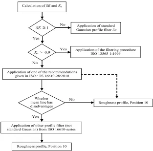
Based on the value of the SE parameter, this paper

proposes an expansion of the current procedure for obtaining the primary profile, the roughness profile, and the waviness profile shown in Fig. 1 using the algorithm shown in Fig. 16. The proposal is to replace Position 9 of Fig. 1 with the algorithm shown in Fig. 16.

6 CONCLUSIONS

The new SE parameter has proven to be a successful

attempt to qualitatively determine the status (shape and character) of primary profiles. An SE value of one was shown to be a significant value from the point of view of filtration using a Gaussian filter. For

primary profiles where the value of SE is less than

(9)

the standard Gaussian filter should not be expected, and vice versa.

These investigations propose a new approach to the determination of surface roughness, where the choice of the most appropriate profile filter directly depends on the shape of the primary profile. This paper proposes that the shape of the primary profile should be determined quantitatively, instead of qualitatively (as is the current practice), using the new parameter of statistic equality of sampling lengths SE.

The calculated values for Psk and Pku showed

that there is no dependence between the Gaussian nature of the primary profiles and the new parameter SE, since there is no dependency between the Gaussian nature of the primary profiles and the disadvantages of using the filter mean lines.

The SE parameter can also be used as a tool for providing information about the stability of the production process. If the surface topography is constituted within a stable production process, then the irregularities will be accumulated around the mean line (value).

An increased value of the SE parameter may, in some cases, indicate the following:

- Fig. 14 indicates the use of an inappropriate method for removing the shape from the total profile;

- Inappropriate selection of the sampling length: In spite of the recommendations provided in [25] for the selection of the sampling length value depending on the form (character) of the profile, the selection can be an inappropriate selection if the profile is of a combined character and there are difficulties with the classification of the profile, i.e. it is unclear whether it belongs to non-periodic or non-periodic profiles.

In the future, it would be significant to investigate the dependence of the parameter SE on:

- The differences in the shape of the primary profiles and their parameters obtained from two different measuring instruments that have different mechanical references.

- Since the parameter SE is calculated for the primary profile, i.e. after the levelling of the total profile, it can be used as a parameter for comparing the various methods of levelling.

Calculation of SE and Ks

Application of the filtering procedure ISO 13565-1:1996

Yes No

Roughness profile, Position 10

Application of other profile filter (not standard Gaussian) from ISO 16610-series

Whether mean line has disadvantages

Application of standard Gaussian profile filterλc

Yes

Ks > 0.9

Application of one of the recommendations given in ISO / TS 16610-28:2010

No

Yes

SE 1

(10)

7 REFERENCES

[1] Jiang, X., Scott, P.J., Whitehouse, D.J., Blunt, L. (2007). Paradigm shifts in surface metrology. Part I. Historical philosophy. Proccedings of the Royal Society, vol. 463, p. 2049-2070, DOI:10.1098/rspa.2007.1874.

[2] Jiang, X., Scott, P.J., Whitehouse, D.J., Blunt, L. (2007). Paradigm shifts in surface metrology. Part II. The current shift. Proccedings of the Royal Society, vol. 463, p. 2071-2099, DOI:10.1098/rspa. 2007.1873. [3] Stanisław, A., Edward, M., Čuš, F. (2009). A model

of surface roughness constitution in the metal cutting process applying tools with defined stereometry.

Strojniški vestnik - Journal of Mechanical Engineering,

vol. 55, no. 1, p. 45-54.

[4] Edward, M., Łukasz, N. (2012). Analysis and

verification of surface roughness constitution model after machining process. Procedia Engineering, vol. 39, p. 395-404, DOI:10.1016/j.proeng.2012.07.043.

[5] ISO 4287:1997. Geometrical Product Specifications

(GPS) - Surface texture: Profile method - Terms, definitions and surface texture parameters. International Organization for Standardization, Geneva.

[6] ISO 3274:1996. Geometrical Product Specifications

(GPS) - Surface texture: Profile method - Nominal characteristics of contact stylus instruments.

International Organization for Standardization, Geneva. [7] ISO 11562:1996. Geometrical Product Specifications

(GPS) - Surface texture: Profile method - Metrological characteristics of phase correct filters. International Organization for Standardization, Geneva.

[8] ASME B46.1 (2009). Surface Texture (Surface

Roughness, Waviness, and Lay). The American Society of Mechanical Engineers, New York.

[9] Raja, J., Muralikrishnan, B., Fu, S. (2002). Recent advances in separation of roughness, waviness and form. Journal of the International Societies for Precision Engineering and Nanotechnology, vol. 26, no. 2, p. 222-235, DOI:10.1016/S0141-6359(02)00103-4.

[10] Whitehouse, D.J. (2011). Handbook of Surface and Nanometrology, Second edition. CRC Press, Taylor & Francis Group, Boca Raton, USA.

[11] Muralikrishnan, B., Raja, J. (2009). Computational

Surface and Roughness Metrology. Springer, London. [12] ISO 13565-1:1996. Geometrical Product Specifications

(GPS) - Surface texture: Profile method; Surfaces having stratified functional properties - Part 1: Filtering and general measurement conditions.

International Organization for Standardization, Geneva.

[13] ISO 16610-21:2011. Geometrical product

specifications (GPS) - Filtration: Linear profile filters: Gaussian filters. International Organization for Standardization, Geneva.

[14] ISO/TS 16610-28:2010. Geometrical product

specifications (GPS) – Filtration - Part 28: Profile filters: End effects. International Organization for Standardization, Geneva.

specifications (GPS) - Filtration: Robust profile filters: Gaussian regression filters. International Organization for Standardization, Geneva.

specifications (GPS) - Filtration: Robust profile filters: Spline filters. International Organization for Standardization, Geneva.

specifications (GPS) - Filtration: Linear profile filters: Spline filters. International Organization for Standardization, Geneva.

specifications (GPS) - Filtration: Linear profile filters: Spline wavelets. International Organization for Standardization, Geneva.

specifications (GPS) - Filtration: Morphological profile filters: Disk and horizontal line-segment filters.

International Organization for Standardization, Geneva.

specifications (GPS) - Filtration: Morphological profile filters: Scale space techniques. International Organization for Standardization, Geneva.

[21] Wozencraft, J.M., Jacobs, I.M. (1965). Principles of communication engineering. John Wiley & Sons, New York, London, Sydney.

[22] ISO 13565-3:1998. Geometrical Product Specifications (GPS) - Surface texture: Profile method; Surfaces having stratified functional properties - Part 3: Height characterization using the material probability curve.

International Organization for Standardization, Geneva. [23] Bury, K. (1999). Statistical distributions in engineering.

Cambridge University Press, Cambridge, DOI:10.1017/ CBO9781139175081.

[24] Taylor, J.K., Cihon, C. (2004). Statistical techniques for data analysis (Second edition). Chapman & Hall/ CRC Press, Boca Raton, USA.

[25] ISO 4288:1996. Geometrical product specifications

(GPS) - Surface texture: Profile method - Rules and procedures for the assessment of surface texture.