The Unconditional and Conditional Methods to Examine the Weekend Effect of Stock Returns

(1)

Issues

ISSN: 2146-4138

available at http: www.econjournals.com

International Journal of Economics and Financial Issues, 2015, 5(Special Issue) 412-419.

2nd AFAP INTERNATIONAL CONFERENCE ON ENTREPRENEURSHIP AND BUSINESS MANAGEMENT (AICEBM 2015), 10-11 January 2015, Universiti Teknologi Malaysia, Kuala Lumpur, Malaysia.

The Unconditional and Conditional Methods to Examine the

Weekend Effect of Stock Returns

Suwandi

1

_{, M. Dileep Kumar}

2

_{, Saqib Muneer}

3

_*

1_{Center of Postgraduate Studies, Cenderawasih University, Jayapura, Papua, Indonesia,}2_{University Institute for International and}

European Studies, University Gorgasali, Georgia, 3_{Faculty of Management, Universiti Teknologi Malaysia.}

*Email: [email protected]

ABSTRACT

This paper examines the weekend effect on stock market returns by using the unconditional method and the conditional method. This paper uses

daily closing prices of firms listed in Indonesian stock exchange by using LQ-45 index from January 2006 to December 2013 in three subperiods: All months, non-January months and January month. Independent sample t-test is applied to examine the significance of the weekend effect. Results support

the weekend effect in three subperiods by using the unconditional method. But when using the conditional method, the weekend effect only exists in down market for all months period and non-January months period. There’s no weekend effect in January month period by using the conditional

method, both in up and down market. This paper presents new evidences and supplements the finance literature on the weekend effect for the case in

Indonesian stock exchange, and also help investors to develop a good investment strategy.

Keywords: Weekend Effect, The Conditional Method, The Unconditional Method, Return of Stock JEL Classifications: E44, G1

1. INTRODUCTION

Information is one of the key factor for an investor in the capital

market. Efficient market is defined as one in which the prices of securities quickly and fully reflect all available information about the assets (Jones, 2004). According to the efficient market, prices

of securities are assumed random, not patterned, and unpredictable. Market anomalies are in contrast to what would be expected in a

totally efficient market. Numoreus empirical studies have indicated

persistent and potentially exploitable weekend effect and January effect in stock returns in many countries.

The first study of weekend effects in security markets appeared in

the Journal of Business in 1931, written by Fields (1931). Fields didn’t use statistical tests, but many researchers interested in the

same field of research. French (1980) continued this direction of research and was the first author to employ statistical methods

in order to test for the existence of the calendar effects. There’re

many other studies about weekend effect anomaly, which referred tothe negative Monday returns and the positive Friday returns (Chen et al, 2008; Cinko and Afci, 2009; and Kamath and Liu, 2011). However, various studies on market anomalies notoccured only on Monday and Friday, but also occured on other days. There’re negative returns on Tuesday (Raj and Kumari, 2006). Elango and Al Macki (2008) found the lowest returns were on Monday and Friday, whereas the highest returns were on Wednesday. Tachiwou (2010) found the lowest returns were on the middle of the week, Tuesday and Wednesday, and a higher pattern towards the end of the week, Thursday and then Friday. Derbali and Khadraoui (2011) found negative returns on Wednesday and positive returns on Friday. Darrat et al., 2013 found Monday effect and Tuesday effect, whereby the

returns on Monday and Tuesday were significantly lower than the

return on the benchmark day of Wednesday.

Market anomaly also appears on January month, it’s called

(2)

effect. Since this discovery, many studies that examined this market anomaly. Other researchers that supported the existence of January effect were Kato and Challhei (1985); Choudhry (2001); Al-Rjoub and Alwaked (2010); and Guler (2013). Market anomalies also appear on other months. Ahsan and Sarkar (2013)

found June Effect in Bangladesh, whereby there were significant positive returns on June. However, in contrast to the findings from

Nageswari et al., 2013, they found the highest returns were on December and the lowest returns were on January. Ogieva et al., 2013 found negative returns were on February, March, April, May and December. Wheras positive returns were on January, August, September, October and November.

Stock prices in the stock market will always fluctuate. Fluctuations

in market can occur whether in up or down market. For a rational

investor, that fluctuations must be faced with a good investment

strategy to obtain the optimal returns at a certain level of risk that is able to be carried. This study will also test the weekend effect without differentiated market (the unconditional method) and differentiated market (the conditional method). So far, no studies have examined more comprehensively about the capital market anomalies, namely weekend effect, with three subperiods for the test: All months, non-Januarymonths and January month, using the unconditional method and the conditional method in companies

listed in the LQ-45 index in Indonesian stock exhange.

2. LITERATURE REVIEW

Weekend effect is used to describe the phenomenon in financial markets in which stock returns on Monday are often significantly

lower than those of the immediately preceding Friday (Singhal and Bahure, 2009). Weekend effect anomaly is contrary to the theory

of market efficiency. This anomaly is appealing to be examined

because the presence of weekend effect can be useful as a trading

strategy that can gain profits for investors. Investors could buy

stocks on days with abnormally low returns and sell stocks on days with abnormally high returns (Tachiwou, 2010). Fields (1931) examined the pattern of the Dow Jones Industrial Average (DJIA) for the period 1915-1930. He compared the closing price of the DJIA for Saturday with the mean of the closing prices on Friday and Monday. For the 717 weekends he studied, the Saturday prices were more than $10 higher than the Friday-Monday mean. French (1980) continued this direction of research and was the

first author to employ statistical methods in order to test for the

existence of the calendar effects. He used the S and P 500 index to study daily returns and obtained similar results. He studied the period 1953-1977 and found that the mean Monday returns were negative for the full period and also for every 5 year sub-period. The mean returns were positive for all other days of the week, with Wednesdays and Fridays having the highest returns. Lin and Chen (2008) found the weekend effect in the Taiwan mutual fund market in period January 1986 to June 2006. The results revealed

significantly negative Monday returns and positive Friday returns.

This weekend effect did not vary greatly between the early and later periods of the month. Cinko and Afci (2009) used the data in Istanbul stock exchange from ISE-100 index. The data set was composed of daily returnsfor 324 stockstraded in ISE and market capitalization based portfolio returns during 1995-2008. By the

use of regression model, they found significant negative Monday returns and significant positive Thursday and Friday returns.

Kamath and Liu (2011) examined the daily return data on the market index, IPSA, of the Santiago stock exchange of Chile.

By using the regression model, in the first sub-period (January,

2003-October, 2005), there was the traditional Monday-Friday pattern, in the second sub-period (November 2005 – Agustus 2008), the anomaly effect was attributable to the significantly positive

Wednesday returns.

However, various studies on market anomalies were occuredon other days. Raj and Kumari (2006) investigated the presence of seasonal effects in the Indian stock market by the two major indices, the Bombay Stock Exchange Index and the National stock exchange Index. By using the multiple regression model, the results found returns on Monday were positive, returns on Tuesday were negative and January effectwas not found in India. Elango and Al Macki (2008) used the real-time data of the National Stock Exchange of India (NSE) for 1999-2007 period of three of the major indices, S and P CNX Nifty, S and P CNX Defty, and CNX Nifty Junior. Results indicated lower returns on Monday and Friday. Surprisingly, Wednesdays have yielded the maximum returns across indices. Tachiwou (2010) investigated daily stock market anomalies by using daily opening and closing values for the two stock Index of West African regional markets from September 1998 to December 2007. The two indexes were Brvm-10 index and Brvm-composite index. A pattern of lower returns around the middle of the week, Tuesday and then Wednesday; and a higher pattern towards the end of the week, Thursday and then Friday, were observed. Derbali and Khadraoui (2011) used the data of Morocco Exchange Market for 74 companies. The results

showed that Friday was a statistically significant positive return on assets. While that on Wednesday was a statistically significant

negative return on assets. Darrat et al., (2013) examined seasonal anomalies in Johannesburg daily stock returns from January 1973 to September 2012. They found no compelling evidence for either a January or December effect in the South African market.

Returns on Monday and Tuesday were significantly lower than

thereturns on the benchmark day of Wednesday. Nevertheless, these strongseasonal effects disappeared in thepost-2008 period

following the global financial crisis.

Market anomalies also occur in January month, whereby stock prices tend to fall towards the end of December and then recuperate quickly in the 1st_{month of the New Year, January (Ahsan and}

Sarkar, 2013). Wachtel (1942) was the first to examine January

(3)

War I period using the data from January 1870 to December 1913 in Germany and the UK and from January 1871 to December 1913 for the US. The empirical research was conducted using a non-linear GARCH-t model. Results obtained provide evidence of the January effect and the month of the year effect on the UK and US returns. There was month of the year anomaly, but there was no January effect in German returns. Al-Rjoub and Alwaked (2010) used the data from the DJIA, the Standard and Poors 500 (S and P 500) and the National Association of Securities Dealers

Automated Quotations indices by using ordinary least square

regression, this paper found that the average January returns were consistently negative during crises. They also found that average loss in returns of January during crises were much smaller than average loss in returns during other months of the crises. Guler (2013) found January effect in China, Argentina and Turkey returns. However no evidence of a January effect was found at Brazil and India stock markets.

Market anomalies also occur in other months. Ahsan and Sarkar (2013) examined the existence of January effect in Dhaka Stock Exchange (DSE) in Bangladesh. Regression model combined with dummy variables and monthly DSE All Share price index from January 1987 to November 2012 has been used to test January effect in the stock return in DSE. It was empirically found that, although January anomaly didn’t exist in DSE, there

was significant positive return in June. Nageswari et al. (2013)

found that the highest mean return was earned in December and the lowest/negative mean return earned in January month for S and P CNX Nifty index. The S and P CNX 500 index recorded the highest mean return in the month of March and the highest negative mean returns in the month of January. The analytical results of seasonality indicated the absence of January anomaly during the study period. Ogieva et al., (2013) examined the calendar effect in the Nigerian Stock Market from 19 April 2005 to 30 September 2010. Using the multiple ordinary least square regression, they found negative returns on Monday, Thursday and Friday. They also found positive returns on Tuesday and Wednesday. Returns in February, March, April, May and December were negative

significant. Wheras the positive returns appeared in January,

August, September, October and November. In the case of June and July there were mixed signs.

3.

THE METHODOLOGY

This paper uses weekly data, every Monday and Fridayin period 2006-2013 and it is divided into 3 subperiods: All months, non-January months and non-January month. By using purposive sampling,

this paper has 12 firms that continued listing in LQ-45 Index in

Indonesian stock exchange.

Dependent variable in this paper is return of stock, calculated as:

Ri(t) =

P P

P

i(t) i(t-1)

i(t-1)

-Where Ri(t) is return on stock i at time t; Pi(t) is price on stock i at

time t; P_i(t-1)is price on stock i at time t-1. Independent variables

in this paper are weekend effect. Weekend effect refers to the abnormally high returns to common stocks on Friday and negative returns on Monday. This paper uses the unconditional method and the conditional method (Pettengill et al., 1995). The unconditional method is a method without dividing the market conditions, wheras the conditional method is a method with dividing the market conditions, up and down market. Up market is whenthere is a positive risk premium (Rm - Rf) > 0 dan down market is when there is a negativerisk premium (Rm - Rf) < 0. Where Rm refers to return of market and Rf refers to return of risk free rate. The hypotheses in this paper are:

Ho: The average return on Monday is the same to the average return on Friday.

Ha: The average return on Monday is different to the average return on Friday.

Before testing the significance of differences between return on Monday and return on Friday, first it can be found if there is

weekend effect in each of the subperiods, where the mean return on Monday is lower than the mean return on Friday. Next, the

significance of differences should be investigated. In testing the

hypothesis, this study will use the independent sample t-test. If

the probability of significance ≤ 0.05, Ho is rejected, that means

the average return on Monday is different to the average return on

Friday. If the probability of significance > 0.05, Ho is accepted, that

means the average return on Monday is the same to the average return on Friday.

4. RESULTS AND DISCUSSIONS

4.1. All Months Period by Using the Unconditional Method

Table 1 shows that the average return on Monday is –0.0015, lower than the average return on Friday, 0.0011.

The probability of significance in Levene’s test for equality of variances is 0.000 ≤ 0.05, that means the variance is different.

Thus the t-test analysis is using equal variances not assumed.

The probability of significance in equal variances not assumed is

0.001 (two-tailed). So it can be concluded that there is weekend effect, whereas the average return on Monday is lower than the average return on Friday, and the average difference on Monday

and Friday is significant different (the probability of significance 0.001 ≤ 0.05) (Table 2).

4.2. All Months Period by Using the Conditional Method (up Market)

Table 3 shows that the average return on Monday is 0.0137, higher than the average return on Friday, 0.0104.

The probability of significance in Levene’s test for equality of variances is 0.005 ≤0.05, that means the variance is different.

Thus the t-test analysis is using equal variances not assumed. The

probability of significance in equal variances not assumed is 0.000

(4)

return on Friday, eventhough the average difference on Monday

4.3. All Months Period by using the Conditional Method (down Market)

Table 5 shows that the average return on Monday is −0.0149, lower than the average return on Friday,−0.0116, or in other words,

theaverage loss in return of Monday is bigger than Friday.

4.4. Non-January Months Period by Using the Unconditional Method

Table 7 shows that the average return on Monday is −0.0007,

lower than the average return on Friday, 0.0011.

Table 1: Group statistics

Day N Mean SD SEM

Return

Monday 4677 –0.0015 –0.04593 –0.00067

Friday 4500 –0.0011 –0.02800 –0.00042

SD: Standard deviation, SER: Standard error mean

Return

Monday up 2299 0.0137 0.03599 0.00075

Friday up 2601 0.0104 0.02635 0.00052

SD: Standard deviation, SER: Standard error mean

Return

Monday down 2367 –0.0149 0.03281 0.00067

Friday down 1899 –0.0116 0.02507 0.00058

SD: Standard deviation, SEM: Standard error mean

Table 2: Independent samples test

t-test for Levene’s test for

equality of variances t-test for equality of means

F Significant t df Significant

(two-tailed) differenceMean Standard error difference 95% CI of the differenceLower Upper Return

Equal variances assumed 35.124 0.000 –3.277 9175 –0.001 –0.00261 0.00080 –0.00418 –0.00105 Equal variances not assumed –3.306 7779.361 0.001 –0.00261 0.00079 –0.00416 –0.00106 CI: Confidence interval

Equal variances assumed 7.817 0.005 3.639 4898 0.000 0.00325 0.00089 0.00150 0.00501

Equal variances not assumed 3.571 4164.844 0.000 0.00325 0.00091 0.00147 0.00504

(5)

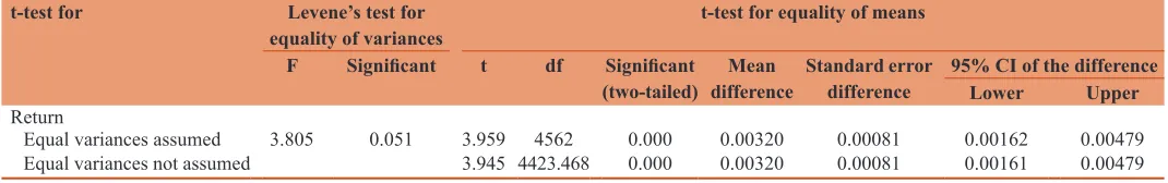
4.5. Non-January Months by Using the Conditional Method (up Market)

The probability of significance in Levene’s test for equality of

variances is 0.051 > 0.05, that means the variance is the same. Thus the t-test analysis should use equal variances assumed. The

probability of significance in equal variances assumed is 0.000

(two-tailed). So it can be concluded that there is no weekend effect, whereas the average return on Monday is higher than the average return on Friday, eventhough the average difference on

Monday and Friday is significant different (the probability of significance 0.000 ≤ 0.05) (Table 10).

4.6. Non-January Months Period by Using the Conditional Method (down market)

Table 11 shows that the average return on Monday is –0.0147, lower than the average return on Friday, –0.0116, or in other words, average loss in returns of Monday is bigger than Friday.

Thus the t-test analysis should use equal variances not assumed.

0.001 (two tailed). So it can be concluded that there is weekend effect, whereas the average return on Monday is lower than the average return on Friday, and the average difference on Monday

Return

Monday non-January 3791 −0.0007 0.03383 0.00055

Friday non-January 4140 0.0011 0.02798 0.00043

Return

Monday non-January up 2154 0.0135 0.02819 0.00061

Friday non-January up 2410 0.0103 0.02641 0.00054

Equal variances assumed 3.805 0.051 3.959 4562 0.000 0.00320 0.00081 0.00162 0.00479

Equal variances not assumed 3.945 4423.468 0.000 0.00320 0.00081 0.00161 0.00479

CI: Confidence interval

Equal variances assumed 13.936 0.000 −2.643 7929 0.008 −0.00184 0.00069 −0.00320 −0.00047

Equal variances not assumed −2.621 7374.977 0.009 −0.00184 0.00070 −0.00321 −0.00046

(6)

4.7. January Months Period by Using the Unconditional Method

Table 13 shows that the average return on Monday is –0.0116, lower than the average return on Friday, 0.0012.

The probability of significance in Levene’s test for equality of variances is 0.000 ≤ 0.05, that means the variance is

different. Thus the t-test analysis should use equal variances

not assumed. The probability of significance in equal variances

not assumed is 0.031 (two-tailed). So it can be concluded that there is weekend effect although in January month, whereas the average return on Monday is lower than the average return on Friday, and the average difference on Monday and Friday

is significant different (the probability of significance 0.031 ≤

0.05) (Table 14).

4.8. January Months Period by Using the Conditional Method (up market)

Thus the t-test analysis should use equal variances not assumed.

The probability of significance in equal variances not assumed

is 0.586 (two tailed). So it can be concluded that there is no weekend effect, whereas the average return on Monday is higher than the average return on Friday, and the average difference on

Monday and Friday is not significant different (the probability of significance 0.586 > 0.05) (Table 16).

Return

Monday non-January down 2129 −0.0147 0.03211 0.00070

Friday non-January down 1730 −0.0116 0.02497 0.00060

Return

Monday non-January 394 −0.0116 0.11353 0.00572

Friday non-January 360 0.0012 0.02828 0.00149

Return

Monday non-January up 145 0.0166 0.09371 0.00778

Friday non-January up 191 0.0122 0.02550 0.00184

(7)

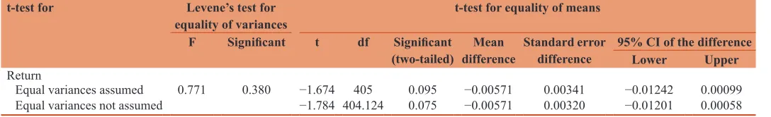
4.9. January Months Period by using the Conditional Method (down Market)

Table 17 shows that the average return on Monday is –0.0170 lower than the average return on Friday, –0.0113, or in other words, average loss in returns of Monday is bigger than Friday.

The probability of significance in Levene’s test for equality of

variances is 0.380 > 0.05, that means the variance is the same. Thus the t-test analysis should use equal variances assumed.

The probability of significance in equal variances not assumed

is 0.095 (two tailed). So it can be concluded that there is no weekend effect, because the average difference on Monday and

Friday is not significant different (the probability of significance

0.095 > 0.05) (Table 18).

5.

CONCLUSIONS AND RECOMMENDATIONS

Results support the weekend effect in three subperiods by using the unconditional method. But when using the conditional method, the weekend effect only appears in down market in all months period and non-January months period. There’s no weekend effect in January month period when using the conditional method, both in up market and down market.This paper presents new evidences

and supplements the finance literature on the weekend effect for

the case in Indonesian stock exchange, and also help investors to develop a good investment strategy. Investors could buy stocks on Monday with abnormally low returns and sell stocks on Friday with abnormally high returns in three subperiodsby using the unconditional method. Investors could also buy stocks on Monday, because the prices on Monday are lower than the prices on Friday in all months period and non-January months period by using the

conditional method in down market, and then sell stocks on Friday in three subperiods by using the unconditional method.

REFERENCES

Ahsan, A.F.M., Sarkar, A.H. (2013), Does january effect exist in Bangladesh?. International Journal of Business and Management, 8(7), 29-35.

Al-Rjoub, S.A.M., Alwaked, A. (2010), January effect during financial

crises: Evidence from the U.S. European Journal of Economics, Finance and Administrative Sciences, 24, 29-35.

Chen, C.Y., Lin, C.J., Lin, Y.C. (2008), Audit partner tenure, audit firm

tenure, and discretionary accruals: Does long auditor tenure impair earnings quality?. Contemporary Accounting Research, 25(2), 415-445.

Choudhry, T. (2001), Month of the year effect and january effect in pre-WWI stock returns: Evidence from a non-Linear GARCH Model. International Journal of Finance and Economics. 6(1), 1-11. Cinko, M., Afci, E. (2009), Examining the day of the week effect in

istanbul stock exchange. The International Business and Economics Research Journal, 8(11), 45-49.

Elango, R., Al Macki, N. (2008), Monday effect and stock return seasonality: Further empirical evidence. The Business Review, Cambridge, 10(2), 282-288.

Darrat, A.F., Li, B., Chung, R. (2013), Seasonal anomalies: A closer look at the johannesburg stock exchange. Contemporary Management Research, 9(2), 155-168.

Derbali, A., Khadraoui, N. (2011), Day of the week effect on assets return: Case of the stock exchange of casablanca. Interdisciplinary Journal of Contemporary Research in Business, 3(3), 1244-1255.

Fields, M.J. (1931), Stock prices: A problem in verification. The Journal

of Business of the University of Chicago, 4(4), 415-418.

French, K.R. (1980), Stock returns and the weekend effect. Journal of

Return

Monday non-January down 238 −0.0170 0.03853 0.00250

Friday non-January down 169 −0.0113 0.02606 0.00200

Equal variances assumed 4.626 0.032 0.615 334 0.539 0.00437 0.00710 −0.00960 0.01833

Equal variances not assumed 0.546 160.260 0.586 0.00437 0.00800 −0.01143 0.02016

Equal variances assumed 0.771 0.380 −1.674 405 0.095 −0.00571 0.00341 −0.01242 0.00099

Equal variances not assumed −1.784 404.124 0.075 −0.00571 0.00320 −0.01201 0.00058

(8)

Financial and Economics, 8(1), 55-69.

Guler, S. (2001), January effect in stock returns, evidence from emerging markets. Interdisciplinary Journal of Contemporary Research in Business, 5(4), 641-648.

Jones, C.P. (2004), Investments: Analysis and Management. 9th_{ed. United}

States of America: John Wiley & Sons, Inc.

Kamath, R., Liu, C. (2011), The day-of-the-week effect on the santiago stock exchange of chile. Journal of International Business Research, 10(1), ???.

Kato, K., Schallheim, J.S. (1985), Seasonal and size anomalies in the

Japanese stock market. The Journal of Financial and Quantitative

Analysis, 20(2), 243-260.

Lin, M.C. (2008), The profitability of the weekend effect: Evidence from

the Taiwan mutual fund market. Journal of Marine Science and Technology, 16(3), 222-233.

Nageswari, P., Selvam M., Vanitha, S., Babu, M. (2013), An empirical analysis of january anomaly in the Indian stock market. International Journal of Accounting and Financial Management

AQ4

Research, 3(1), 177-186.

Ogieva, O.F., Osamwonyi, I.O., Idolor, E.J. (2013), Testing calendar effect on nigerian stock market returns: Methodological approach. Journal of Financial Management and Analysis, 33, 277-282.

Pettengill, G.N., Sundaram, S., Mathur, I. (1995), The conditional relation

between beta and returns. Journal of Financial and Quantitative

Analysis, 30(01), 101-116.

Raj, M., Kumari, D. (2006), Day-of-the-week and other market anomalies in the indian stock market. International Journal of Emerging Markets, 1(3), 235-246.

Singhal, A., Bahure, V. (2009), Weekend effect of stock returns in the indian market. Great Lakes Herald, 3(1), 12-22.

Tachiwou, A.M. (2010), Day-of-the-week-effects in west African regional stock market. International Journal of Economics and Finance, 2(4), 167-173.

Wachtel, S.B. (1942), Certain observations on seasonal movements in stock prices. The Journal of Business of the University of Chicago, 15(2), 184-193.

Author Query???