Cho06

(1)

Computing, Artiﬁcial Intelligence and Information Technology

A tandem clustering process for multimodal datasets

Catherine Cho, Sooyoung Kim

*

_{, Jaewook Lee, Dae-Won Lee}

Department of Industrial Engineering, POSTECH (Pohang University of Science & Technology), Hyoja San 31, Pohang 790-784, South Korea

Received 19 March 2003; accepted 13 May 2004 Available online 7 August 2004

Abstract

Clustering multimodal datasets can be problematic when a conventional algorithm such ask-means is applied due to its implicit assumption of Gaussian distribution of the dataset. This paper proposes a tandem clustering process for multimodal data sets. The proposed method first divides the multimodal dataset into many small pre-clusters by apply-ingk-means or fuzzyk-means algorithm. These pre-clusters are then clustered again by agglomerative hierarchical clus-tering method using Kullback–Leibler divergence as an initial measure of dissimilarity. Benchmark results show that the proposed approach is not only effective at extracting the multimodal clusters but also efficient in computational time and relatively robust at the presence of outliers.

Keywords:Multivariate statistics; Artiﬁcial intelligence; Clustering; Multimodal dataset;K-means algorithm

1. Introduction

A number of clustering algorithms have been developed by many researchers in different areas of applications and many studies are still being carried out to develop the ways to find appropriate and meaningful clusters from given data. Such abundance and diversification of clustering algo-rithms indicate the necessity of developing

algorithms speciﬁc for certain data characteristics. There seems to be no one universal method of clus-tering which suits every type of datasets and ﬁnds the right clusters in every application. Thus, the development of clustering algorithms is usually bounded within certain data characteristics as it is the case in this study.

This study presents a method called tandem clustering process (TCP) designed for data with multimodal or non-Gaussian distributions within clusters. The proposed TCP is constituted of con-ventional k-means and hierarchical clustering algorithms with Kullback–Leibler divergence as an initial measure of dissimilarity followed by the

*

Corresponding author. Fax: +82 54 2792870. E-mail address:[email protected](S. Kim).

(2)

group-average linkage method. By usingk-means algorithm in the first step of generating pre-clus-ters, the effect of outliers is lessened and the com-putational time is reduced compared to running a hierarchical clustering algorithm alone. Secondly, the implementation of Kullback–Leibler (K–L) divergence into the hierarchical method could ex-tract the clusters with multimodal distributions more effectively.

In the following section, two major types of clustering algorithms are reviewed. The steps of the proposed TCP method are described in Section 3 along with the brief introductions of k-means algorithm and K–L divergence. An illustrative example of the proposed method is given in Sec-tion 4. SecSec-tion 5 gives the result of computaSec-tional tests on diﬀerent datasets. Finally, the conclusions are given in Section 6.

2. Background and review

Many algorithms and methods have been devel-oped under the eﬀort of mining meaningful infor-mation from a dataset by means of clustering. Those algorithms can be grouped according to their mathematical basis or the basic concept be-hind them. Two major branches of the conven-tional clustering techniques are hierarchical clustering and non-hierarchical algorithms such ask-means and fuzzyk-means method. Since our proposed method tries to resolve some of the dis-advantages that conventional hierarchical and k -means algorithm have, the current section is devoted to a brief survey on hierarchical and

k-means clustering algorithms.

The basis of hierarchical clustering is a cluster hierarchy whereas the essence of the algorithms is to build a tree structure from the data. The algo-rithms for building a tree from top to bottom, con-sidering all of the data points to be one cluster, are called hierarchical divisive clustering methods and the algorithms using bottom-up method are called hierarchical agglomerative clustering methods. The current survey is focused on the hierarchical agglomerative clustering (HAC) algorithms which are among the oldest and most popular clustering methods.

HAC algorithms start withNnumber of single data-point clusters and merge a pair of clusters that are closest to one another (or most similar to one another) recursively. After a single merge, new distances (or dissimilarities or similarities) be-tween all pairs of clusters are re-calculated before the next merge. The process is repeated until a stopping criterion is satisﬁed or all data points are merged into a single cluster. The hierarchical structures of the clusters are represented in the form of dendrograms.

One of the most critical issues in HAC is the measure of dissimilarity between pairs of clusters called linkage metrics. A number of linkage met-rics with the subsequent HAC algorithms have been developed. The linkage metrics can be subdi-vided into graphic metrics and geometric metrics as described in Dash et al. [4]. Single, complete, and average linkage are included in graphic meth-ods considering each point in a cluster to be its representative, whereas centroid, median, and WardÕs linkage are geometric metrics representing a cluster by its central point [2].

The early algorithms proposed by Sibson imple-mented single linkage as a measure of dissimilarity (or distance) between clusters where the distance between two clusters is represented by the mini-mum distance between any two points, one from each cluster [22]. The complete linkage used in the algorithm proposed by Defays [6] uses the maximum distance to be the representative dis-tance between two clusters. VoorheeÕs method

[24]is based on the average link where the dissimi-larity is measured as the average distance between any pair of points, one from each cluster.

(3)

using the objective function ofk-means, which will be mentioned in Section 3.1. Current study applies Kullback–Leibler divergence as an initial dissimi-larity measure between clusters which is discussed in detail in Section 3.2.

All of the discussed linkage methods used in hierarchical clustering have their base on the Lance–Williams scheme[14]which has the updat-ing formula as

dðk;i[jÞ ¼dði[j;kÞ

¼aðiÞdðk;iÞ þaðjÞdðk;jÞ

þcjdðk;iÞ dðk;jÞj: ð1Þ

This equation shows that the distance (dissimilar-ity) between the cluster k and the merged cluster ofiandjcan be calculated in terms of the distance between cluster i and kand the distance between cluster j and k. The a(i) and a(j) are constants which depend on cluster i and j whereas c is an arbitrary constant. The linkage metrics can be ver-iﬁed to be instances of this formula depending on the values of the constants[21].

Two major disadvantages of hierarchical clus-tering algorithms are the eﬀect of outliers and the computational complexity. Since most of the algo-rithms do not reconsider the sub-clusters for the purpose of improvement once they were merged in previous steps, the presence of outliers in the wrong place can cause low accuracy in construct-ing the hierarchical structure of the dataset. For example, a few outliers located in between two dis-tinct clusters can act as a bridge merging parts from the two clusters and thus, result in the wrong assignment of clusters[7].

Secondly, most of the traditional HAC algo-rithms suﬀer from time and memory complexity because they search through every pair of clusters to ﬁnd the shortest distance (dissimilarity). When clustering the dataset with N data points and dimension, d, into c clusters using single linkage method, the process requires O(N2) of memory space due to the storage of dissimilarity matrix and O(cN2d2) of time complexity [7]. Another example of high computational cost of HAC is presented in Dash et al.[4]showing that the tradi-tional algorithms using centroid linkage exhibit

O(N3) of computation time. A more eﬃcient algo-rithm for centroid method, called priority queue algorithm suggested by Day and Edelsbrunner[5]

slightly reduces the time complexity to O(N2logN)

[4].

Several studies have been carried out to over-come the disadvantages of HAC. Olson [17]tried to reduce the computational time by parallel algorithms. Karypis et al.[13]use dynamic mode-ling in their algorithm called CHAMELEON with consideration of inter-connectivity and relative closeness in the cluster aggregation. Fisher[9] pro-posed an iterative hierarchical clustering algorithm improving the dendrogram structure by revisiting the merged clusters. An algorithm called CURE developed by Guha et al. [10] also takes care of outliers by implementing shrinkage factors and in-creases computational eﬃciency by data sampling and partitioning.

K-means algorithm ﬁrst proposed by Ball and Hall[1]is one of the most popular clustering algo-rithms in many application areas. It directly as-signs each observation to a cluster and each observation belongs to one and only one cluster. As the name ‘‘k-means’’ implicitly indicates, this method groups data points around k number of centroids by assigning an observation to the near-est centroid. Since checking all possible subsets of clustering is impossible, some greedy heuristics are applied as an iterative optimization. Formal deﬁnition ofk-means algorithm is given in Section 3.1.

The major advantage of thek-means algorithm is the comparatively light load of computation. A fast algorithm is especially useful when high dimensional data with large number of data points is being dealt with. However, the solutions found from the conventionalk-means process are bound to be sub-optimal local minima and depend heav-ily on the location of the initial centroids. The k -means algorithm proposed by Hatigan and Wong

(4)

The original k-means algorithm was modiﬁed so as to give more general fuzzy clusters by Dunn

[8] and Bezdek [3]. The fuzzy k-means clustering algorithm tries to minimize a heuristic global cost function which includes a probability term of each observation belonging to each class. Fuzzy

k-means method usually delivers a more stable solution and it is less dependent on the initial con-ditions at the cost of higher computational complexity.

One critical disadvantage of the k-means and fuzzyk-means algorithms comes from their impli-cit assumption of Gaussian distribution of the data points. They tend to group the data points in spherical clusters and are often unsuccessful at detecting clusters with diﬀerent shapes[20]. Thus, our objective is to resolve such problem of missing multimodal nature of datasets by the proposed tandem clustering process (TCP).

3. The proposed method

We propose a simple two-step method called tandem clustering process (TCP) suitable for data with multimodal distribution within clusters. The basic idea is to apply simple k-means or fuzzy k -means algorithm to the raw dataset for identifying someÔpre-clustersÕ. The ﬁrst step would group the data into some small pre-clusters with normal distributions. In the second step, a hierarchical clustering method is applied to the pre-clusters using Kullback–Leibler divergence as a measure of distance for the ﬁrst merge followed by group-average linkage method used in the subsequent merges.

In Section 3.1, k-means algorithm is explained and Section 3.2 introduces the Kullback–Leibler divergence used in the second step of the TCP. The overall steps of the TCP are presented in Sec-tion 3.3.

3.1. K-means algorithm

K-means clustering was developed in order to assign theNobservations to theKclusters in such a way that the following criterion (the error sum of squares of the clustering) is minimized.

ESS ¼X N

i¼1

ðxitCðiÞÞ0ðxitCðiÞÞ;

whereC(i) is the cluster index forith objectxiand

tCis the centroid for clusterC. An iterative descent

algorithm for minimizing ESS is described below as given in Lattin et al. [16].

K-means Clustering Algorithm

1. Initialization: Choose random values for the ini-tial centroidsftigK_i¼1from input space.

2. Cluster assigning: Assign each object xi to the

cluster index of the closest centroid point.

kðxiÞ ¼arg min

j ðxitjÞ 0

ðxitjÞ; j¼1;. . .;K;

wherek(xi) denote the cluster index of a object

xi.

3. Updating centroid: Adjust the centroids ftigK_i¼1

by re-calculating the means of currently assigned clusters.

4. Continuation: Continue the procedure Step 2– Step 3 until no change is observed in the cent-roidsftigK_i¼₁.

The clustering process begins with the initialK

number of centroids and each data point is as-signed to one of the centers of the Kcentroids in such a way as to minimize the objective function. The initial cluster assignment is used to calculate a new set of centroids to minimize the total cluster variance and the data points are re-assigned to the center of the new centroids minimizing the sum of squared error criterion. This process of calculat-ing centroids and assignment of points is re-peated until the convergence is achieved.

3.2. Kullback–Leibler divergence

Kullback–Leibler divergence, also called rela-tive entropy, is a measure of the diﬀerence between two arbitrary distributions [19]. The general Kull-back–Leibler divergence is written as

DðfjgÞ ¼

Z flogf

g; ð2Þ

(5)

The above equation can be modiﬁed to give symmetric diﬀerence (or distance) between two clusters,k1andk2as

Dðk1;k2Þ ¼

1 2

Z

Rn

pðxjk1Þlog

pðxjk1Þ

pðxjk2Þ

dx

þ1

2

Z

Rn

pðxjk2Þlog

pðxjk2Þ

pðxjk1Þ

dx; ð3Þ

where p(xjk1) and p(xjk2) are the conditional

probability density of x for clusters k1 and k2

respectively[19].

The symmetric Kullback–Leibler distance can be simpliﬁed when two distributions for which the distance is to be measured are assumed to be Gaussian. The simpliﬁed expression of the distance between two clusters with Gaussian distributions derived by Larsen et al. [15]is

D1ðk1;k2Þ ¼

d

2þ 1 4Tr½R

1

k1Rk2 þTr½R

1

k2Rk1

þ1

4ðlk1lk2Þ T

ðR_k₁1þR_k₂1Þðlk1lk2Þ:

ð4Þ

ThelkiandRkirepresent the mean and covariance

matrix of clusterirespectively and a simple Eucli-dean distance between clustersk1andk2is written

asd. Since all clusters in the ﬁrst level of hierarchi-cal clustering can be assumed to follow Gaussian distributions in the TCP method, it is suitable to use the above equation in the ﬁrst step of the hier-archical clustering.

Since the distributions of some clusters are not Gaussian after the initial merge in the hierarchical clustering step, the group-average link method is adopted as a measure of dissimilarity in the subse-quent steps. The group-average link method can also be understood as the weighted K–L distances by the mixing proportions[15]. The group-average link method uses the following distance:

Djþ1ðk;k3Þ ¼

ðPjðk1ÞDjðk1;k3Þ þPjðk2ÞDjðk2;k3ÞÞ

ðPjðk1Þ þPjðk2ÞÞ

:

ð5Þ

This equation approximates the distance between clusterskandk3wherekis the result of the

previ-ous merge of clustersk1andk2. Also,Pj(ki)

repre-sents the priors of the clusterkiat jth level.

3.3. Tandem clustering process (TCP)

As mentioned previously, the proposed tandem clustering process is basically constituted of two widely used methods,k-means (or fuzzyk-means) and the hierarchical clustering method. The ﬁrst part of TCP is to runk-means algorithm with clus-ter number greaclus-ter than the expected number of clusters. This step of producingk0_pre-clusters

seg-regates the small clusters of Gaussian distributions within multimodal clusters. Also, this step could reduce the eﬀect of outliers which can be magniﬁed if running one step hierarchical ork-means algo-rithm alone. The second part of TCP re-groups the k0 _{pre-clusters generated from the previous}

step to capture the multimodal nature of dataset. In this part, the agglomerative hierarchical cluster-ing process is adopted. The detailed steps are given in the following.

Steps of TCP

1. Runk-means or fuzzyk-means algorithm with

k0₌_n_·_k ₍_k0_{= number of the pre-clusters,}

k= the number of expected clusters) and the initial value 2 for multiplier n.

2. Run the ﬁrst step of the agglomerative hierar-chical clustering process using K–L divergence modiﬁed for Gaussian distribution given in Eq. (4).

3. Run the rest of the steps in the agglomerative hierarchical clustering process using group-average link method with the distance given in Eq. (5).

4. Determine the ﬁnal clusters using the hierarchi-cal structure constructed.

5. Compare the current clustering result to the previous one by calculating Rand index to be deﬁned in the later section. (This step is skipped in the ﬁrst iteration.)

6. Repeat steps 1 to 5 increasing n by one until two consecutive results show little diﬀerence in terms of the Rand index (for example, if the index value is greater than or equal to 0.9).

(6)

esti-mate the value ofkwhich is normally unknown at the beginning of the ﬁrst iteration. In such a case, a reasonably big number may be used fork0_{in a trial}

run through steps 1–4, and the resultingkcan be used for the initial clustering of the full TCP.

In step 6, the similarity of the current result to the result of the previous iteration is judged by the Rand index described in Section 5.2. The Rand index is one of the indicators of the similarity be-tween two diﬀerent clustering results with 1.0 (i.e., equivalent results) as the maximum value. The cutoﬀ value of the Rand Index at which the iteration stops may be set depending upon the problem characteristics and the amount of com-puting time allowed.

4. Illustrative example

The step-by-step procedure of TCP is explained in detail with an example ofÔTaegukÕ data shown

in Fig. 1. As presented in the algorithm, TCP is

based upon the iterative search for the best value ofk0_{(pre-clusters) repeating the}_k_{-means and}

hier-archical clustering steps until there is no significant change in the final result. In this illustrative exam-ple, the last iteration will be described assuming the finalk0 _{is already found.}

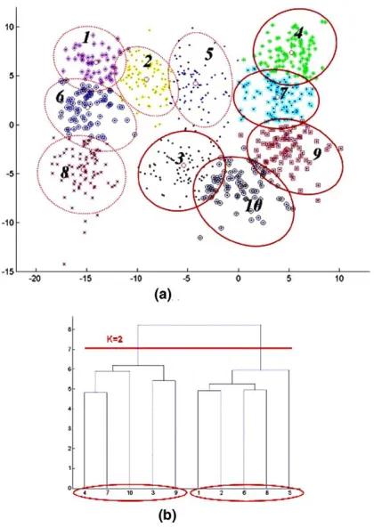
The dataset is clustered byk-means algorithm and 10 pre-clusters are found, i.e.,k0_{= 10, as}

plot-ted in Fig. 2(a). For the case of relatively small

dataset with low variable dimension, fuzzy k -means algorithm is recommended due to its stabil-ity against the location of initial k0_{s. When}

k-means is used for a large dataset instead of fuzzy

k-means algorithm which requires longer compu-tation time, it is recommended to run it several times to diminish the eﬀect of initialk0_s.

Considering the small pre-clusters as individual data points, the ﬁrst merge of agglomerative hierarchical clustering process is carried out with Gaussian-like pre-clusters. The centroids and covariance matrices of the pre-clusters are used to calculate the dissimilarity matrices using symmetric Kullback–Leibler divergence as a measure of dis-tance in the ﬁrst merge. The rest of merges in the hierarchical clustering process are carried out using the group-average link method since the

Fig. 1. Illustrative example of Taeguk data (k= 2 in this case).

(7)

distributions of some clusters are not Gaussian anymore after the ﬁrst merge of pre-clusters. The weighted average method such as group-average linkage is suitable to approximate the dissimilarity between distributions of the data points after the initial merge. The dendrogram generated from the hierarchical clustering step is shown in Fig. 2(b).

Using the hierarchical structure produced, the ﬁnal clusters are determined. The stopping of the merging process or, in other way, horizontal cut-ting of the dendrogram can be carried out accord-ing to the appropriate number of clusters which is either known or expected. In the example ofÔ Tae-gukÕ data, the two clusters are identiﬁed by hori-zontal cutting of the dendrogram as marked in

Fig. 2(b). The numbers in thex-axis of the dendro-gram matches the labels of the pre-clusters on

Fig. 2(a).

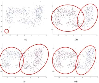
InFig. 3, a set of results obtained by applying

four conventional clustering methods to the same

Taeguk dataset is shown. The red ellipses in the graphs approximately depict the shapes of the identiﬁed clusters to show the diﬀerences from the original clusters. (Note that no overlapping of clusters actually exists in the results.) Prelimi-nary tests to be described in the following section were carried out to test several conventional clus-tering methods on sample datasets.

5. Computational test

The proposed TCP algorithm is implemented in Matlab 6.1 along with some conventional algo-rithms for comparison purpose. In the following sections, tested datasets, performance measure, and the test results are described.

5.1. Datasets

In order to evaluate the eﬀectiveness of the pro-posed TCP, three sample datasets and six publicly

(8)

known datasets were used. The detailed informa-tion of the nine datasets is listed inTable 1 includ-ing the number of observations and the number of clusters as well as the number of dimensions. Since the ﬁrst step of the TCP implementsk-means algo-rithms, the datasets with only continuous variables were used in the simulation.

The six datasets (Balance Scale, Iris, Liver Dis-order, Sonar, Tokyo1, and Waveform 21) were ob-tained from UCI Machine Learning Repository

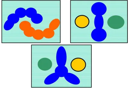
[23]. The datasets obtained from UCI Repository are originally designed for classiﬁcation problems. Of course, the fact is that clustering algorithms are unsupervised methods without known answers. However, for evaluation purpose, we tested with the datasets with known clusters, such as Iris which is often adopted in many clustering prob-lems. In addition to these datasets, three sets of data (Taeguk, Triangle, and Xours as shown in

Fig. 4) were generated according to three

multimo-dal distributions shown ifFig. 5in order to test the eﬃciency of the proposed algorithm. For the pur-pose of simplicity and visualization of the results,

the datasets were generated with two-dimensional variables.

5.2. Rand index

The performance of a clustering algorithm can be assessed by measuring the agreement between the clustering result and the actual answer of the cluster membership. The current study adopted one of the most widely used measures, Rand index, as the performance measure of the tested algo-rithms[18]. It represents the eﬀectiveness of a clus-tering algorithm when the actual target value is known [2]. The calculation of the index starts by selecting a pair of data points and evaluating whether each pair has the same type of cluster membership. It is the ratio of the number of the similar assignments of the point-pairs to the total number of the point-pairs.

Suppose we compare the result from a test algo-rithm against the actual answer known for the

Table 1

Datasets used for the computational tests

Data Name Variable dimension

Number of observations

Number of clusters

Taeguk 2 800 2

Triangle 2 600 3

Xours 2 800 3

Balance scale 4 625 3

Iris 4 150 3

Liver disorder 6 345 2

Sonar 60 208 2

Tokyo1 44 959 2

Waveform 1 21 500 3

Fig. 4. Three generated datasets: (a) Taeguk, (b) Triangle, (c) Xours.

(9)

dataset. We then deﬁne the following numbers for all possible pairs of the data points in the dataset.

a= the number of pairs of data points clustered to be in the same cluster in the algorithm result and also exist in the same cluster in the known answer.

b= the number of data pairs placed in the same class in the answer but clustered to be in diﬀerent classes in the result.

c= the number of pairs placed in the way re-verse to the way that bis deﬁned.

d= the number of pairs of data points that are in diﬀerent clusters for both algorithm result and the actual answer.

The Rand index can be deﬁned as

RI¼total number of similar assignment pairs

total number of point pairs

¼ aþd

aþbþcþd:

ð6Þ

The index value lies between 0 and 1 and has the value of 1 when the two sets of partitions agree perfectly. Obviously, a value closer to 1 would rep-resent a better performed algorithm for the speciﬁc dataset. In simulation, the RI was obtained for all the results and used as a performance measure to evaluate the eﬀectiveness of the proposed algo-rithm. It can be used not only as a performance measure of the obtained result compared to the true result, if available, (Tables 2 and 3) but also as a similarity measure of two consecutive cluster-ing solutions as in step 6 in the proposed TCP if the true result is not available.

5.3. Preliminary clustering using conventional methods

Several conventional clustering algorithms were run to compare their performance to the proposed method. The results of the preliminary test are listed inTable 2for our nine datasets. For

hierar-Table 2

Rand Index values of the preliminary tests applying the conventional algorithms

Taeguk Triangle Xours Balance scale

Iris Liver disorder

Sonar Tokyo1 Waveform 21

Hierarchical-Single 0.4994 0.4451 0.4378 N/A 0.7766 0.5104 0.5006 0.5377 N/A Hierarchical-Complete 0.5283 0.5774 0.7082 N/A 0.8368 0.5104 0.4978 0.5377 N/A Hierarchical-Centroid 0.4994 0.7880 0.6767 N/A 0.8923 0.5050 0.4976 0.5377 N/A Hierarchical-Average 0.7142 0.7920 0.7543 0.5800 0.8923 0.5050 0.5032 0.5377 N/A Hierarchical-Wards 0.7866 0.7148 0.6887 0.6003 0.8797 0.4989 0.4978 0.5681 N/A K-means 0.8118 0.7518 0.7055 0.5885 0.8797 0.5037 0.5014 0.5844 0.6673 Fuzzyk-means 0.8059 0.7589 0.7063 0.5627 0.8797 0.4998 0.5032 0.5987 0.6842

Table 3

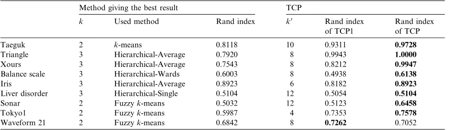
Results of the proposed TCP, TCP1, and the conventional algorithms

Method giving the best result TCP

k Used method Rand index k0 _{Rand index}

of TCP1

Rand index of TCP

Taeguk 2 k-means 0.8118 10 0.9311 0.9728

Triangle 3 Hierarchical-Average 0.7920 8 0.9943 1.0000

Xours 3 Hierarchical-Average 0.7543 8 0.8212 0.9947

Balance scale 3 Hierarchical-Wards 0.6003 8 0.4938 0.6138

Iris 3 Hierarchical-Average 0.8923 6 0.8182 0.8923

Liver disorder 3 Hierarchical-Single 0.5104 12 0.5054 0.5104

Sonar 2 Fuzzyk-means 0.5032 12 0.5123 0.6458

Tokyo1 2 Fuzzyk-means 0.5987 4 0.7353 0.7578

(10)

chical algorithms, four linkage methods such as single, complete, average and Wards were evalu-ated along withk-means, and fuzzyk-means algo-rithm. The performance was measured in terms of the Rand index. The missing RI values substituted byÔN/AÕin the table represent the cases where the given dataset was not analyzed by the speciﬁc algorithms due to high computational complexity.

5.4. Comparison

The proposed TCP was applied to nine datasets and the performance was compared against the conventional algorithms using the Rand index as tabulated inTable 3. The RI values of the conven-tional algorithms were determined by selecting the best value among the conventional approaches ap-plied during the preliminary test. As shown in the ﬁrst three rows of the table, the three generated datasets with distinctive multimodal distributions produced relatively large improvements by TCP in the performance. Also, the RI values of TCP runs on Sonar, Tokyo1 and Waveform 1 exhibited increased performance.

The proposed TCP was also compared against

ÔTCP1Õwhich utilizes the pure group-average clus-tering method in the hierarchical clusclus-tering part of the original TCP (i.e., instead of the K–L diver-gence in Step 2 of TCP, the usual Euclidean dis-tance is used as the dissimilarity measure). The comparison was made to verify the usefulness of the K–L divergence, and the results show that it is in general better, even though the overall diﬀer-ence between the two seems to be rather small. One exception was found for the last dataset, Waveform 21, but the two results are close.

Another beneﬁt found in TCP was its reduction of the computing time, especially when a large dataset was analyzed. Even though there was only a slight improvement in the performance for the dataset Balance Scale and no improvement for Iris and Liver Disorder, the computing times were sig-niﬁcantly smaller compared to the hierarchical methods. The computing burden of TCP seemed to be robust to the changes in the number of dimensions and observations, while the hierarchi-cal algorithms often failed to handle a large data-set within a reasonable amount of computing time.

6. Conclusions

A tandem clustering algorithm termed TCP suitable for clustering the datasets with multimo-dal distributions has been presented in this paper. The major steps of TCP consist of k-means and hierarchical clustering methods. TCP tries to com-bine the strengths of the two methods, and the advantages are the simplicity and the speed of analysis. The computational tests on three gener-ated multimodal datasets and six open datasets demonstrated the performance of TCP. The clus-tering results were compared against those of sev-eral widely known clustering methods and a simple modiﬁcation of TCP itself. In most of the tested cases, TCP outperformed other methods exhibit-ing improvements in both the accuracy of cluster assignment and the computing time.

A further research to ﬁnd the better starting values of the initial number of the pre-clusters would be useful. One may consider the reduction of overall computing time by applying a prudent search of the best value of the number of pre-clusters.

Acknowledgements

The authors would like express the deepest appreciation to the anonymous referees who pro-vided invaluable and detailed comments and edit-ing which signiﬁcantly helped enhancedit-ing the presentation of the paper. This work was sup-ported in part by the Korea Research Foundation under Grant KRF-2003-041-D00608 and in part by BK21 project with POSTECH.

References

[1] G.H. Ball, D.J. Hall, A clustering technique for summa-rizing multivariate data, Behavioral Science 12 (1967) 153– 155.

[2] P. Berkin, Survey of Clustering Data Mining Techniques, Technical Paper, Accure Software, San Jose, CA, 2002. [3] J.C. Bezdek, Numerical taxonomy with fuzzy sets, Journal

of Mathematical Biology 1 (1974) 57–71.

(11)

[5] W.H.E. Day, H. Edelsbrunner, Eﬃcient algorithms for agglomerative hierarchical clustering methods, Journal of Classiﬁcation 1 (1) (1984) 7–24.

[6] D. Defays, Eﬃcient algorithm for a complete link method, The Computer Journal 20 (1977) 364–366.

[7] R.O. Duda, P.E. Hart, D.G. Stork, Pattern Classiﬁcation, Wiley-Interscience, New York, 2001.

[8] J.C. Dunn, A fuzzy relative of the ISODATA process and its use in detecting compact well-separated clusters, Jour-nal of Cybernetics 3 (1974) 32–57.

[9] D. Fisher, Iterative optimization and simpliﬁcation of hierarchical clustering, Journal of Artiﬁcial Intelligence Research 4 (1996) 147–179.

[10] S. Guha, R. Rastogi, K. Shim, Cure: An eﬃcient clustering algorithm for large databases, Information Systems 26 (1) (2001) 35–58.

[11] T. Hastie, R. Tibshirani, J.H. Friedman, The Elements of Statistical Learning: Data Mining, Inference, and Predic-tion, Springer-Verlag, 2001.

[12] J. Hatigan, M. Wong, Algorithm AS136: A k-means clustering algorithm, Applied Statistics 28 (1979) 100–108. [13] G. Karypis, E.H. Han, V. Kumar, Chameleon: A hierar-chical clustering algorithm using dynamic modeling, Com-puter 32 (1999) 68–75.

[14] G. Lance, W. Williams, A general theory of classiﬁcation sorting strategies, Computer Journal 9 (1963) 373–386. [15] J. Larsen, L.K. Hansen, A.S. Have, T. Christiansen, T.

Kolenda, Webmining: Learning from the world wide web,

Computational Statistics & Data Analysis 38 (2002) 517– 532.

[16] J. Lattin, J.D. Carroll, P.E. Green, Analyzing Multivariate Data, Thomson (2003).

[17] C. Olson, Parallel algorithms for hierarchical clustering, Parallel Computing 21 (1995) 1313–1325.

[18] W.M. Rand, Objective criteria for the evaluation of clustering methods, Journal of the American Statistical Association 66 (1971) 846–850.

[19] B.D. Ripley, Pattern Recognition and Neural Network, Cambridge University Press, Cambridge, 1996.

[20] P.J. Rousseeuw, L. Kaufman, E. Trauwaert, Fuzzy clus-tering using scatter matrices, Computational Statistics & Data Analysis 23 (1996) 135–151.

[21] R. Sharan, R. Elkon, R. Shamir, Cluster analysis and its applications to gene expression data, Ernst Schering Res Found Workshop, 2002, pp. 83–108.

[22] R. Sibson, Slink: An optimally eﬃcient algorithm for the single link cluster method, Computer Journal 16 (1973) 30– 34.

[23] UCI Machine Learning Repository. Available from: http://www.ics.uci.edu/~mlearn/MLRepository.html>. [24] E.M. Voorhees, Implementing agglomerative hierarchical