Do the rich consume higher quality goods 170622.pdf

(1)

Do the rich (really) consume higher quality goods?

Evidence from international trade data

Vincenzo Merella

y

_{Daniel Santabárbara}

z

June 2017

Abstract

We provide novel evidence on the relationship between importer income and quality of

imports. Instead of investigating this relationship using import prices as a proxy for product

quality, our approach exploits the di¤erences in quantitative markets shares of products

sourced from distinct exporters to obtain a disaggregated quality measure, within a discrete

choice model where richer consumers demand goods of higher quality. The resulting quality

measure explicitly relates to consumer income, and we test its relationship with income via

a carefully structured panel data. Speci…cally, we treat EU members as distinct consumers

operating in a single market and, exploiting Eurostat’s COMEXT product-level data over

the period 1995-2007, report the existence of a positive link between income and quality that

is robust to a number of di¤erent speci…cations and controls. Based on our estimates, we

also develop a novel quality upgrading indicator that conveniently quanti…es import quality

improvements as importer income rises.

Keywords: import quality, import shares, unit values, nested logit demand

JEL Classi…cations: F12, F14, L15

We would like to thank Henrique Basso, Paola Bertoli, Esteban Jaimovich, Monika Junicke, Pantelis Kazakis, Giovanni Mastrobuoni, Alessio Moro and Miroslav Zajicek for comments and suggestions, as well as seminar participants at the Bank of Spain, the SAEe meeting (Santander), the SIE meeting (Bocconi) and the University of Economics Prague. This paper was written while Vincenzo Merella was a Research Fellow at the Bank of Spain, whose …nancial support is kindly acknowledged.

y_{University of Cagliari and BCAM, University of London. Mailing address: Department of Economics and} Business, Viale Sant’Ignazio 17, 09123 Cagliari, Italy. Email: [email protected].

(2)

1 Introduction

This paper provides novel evidence on the relationship between importer income and quality

of imports. Our objective is to test the link between quality and income departing from the

traditional assumption that information on quality is fully embedded in prices. For this reason,

we infer product quality from prices and market shares within a parsimonious discrete choice

model in which richer consumers demand goods of higher quality. The resulting quality measure

explicitly relates to consumer income. Our empirical exercise exploits this novel feature of our

quality measure, and investigates the quality-income relationship on a panel data, carefully

structured to have a comparable set of products over time and across countries, and at the same

time take importer income heterogeneity into account.

The relationship between product quality and consumer income is a key determinant of

international trade patterns. A number of theoretical contributions show that richer importers

trade more with exporters producing higher quality goods, and this prediction also appears to

…nd support in the empirical literature. The extent to which such empirical …ndings actually

relate to the theoretical prediction is, however, controversial. The crux of the matter is that unit

values (import prices) are typically used as proxies for the quality levels of the imported goods.1

Unit values are calculated at the product level as the ratio between the total value and

the total volume traded from a source country (exporter) to a destination country (importer).

The rationale for using them as proxies for quality hinges on a number of arguments: e.g., higher quality goods would require more costly inputs, hence be more expensive; a market price

di¤erential between two similar goods may hold only if their quality levels di¤er. The correlation

between prices and income may, however, be unrelated to quality, and determined by factors such

as heterogeneous tari¤s and trade costs, pricing-to-market (market-speci…c markups), residual

horizontal di¤erentiation (between close-substitute products).2

1_{Further to establishing the quality-income relationship, the theoretical literature points out that this link} helps in explaining a number of observed regularities: for example, the international product cycle (Flam and Helpman, 1987); the Linder (1961) hypothesis, both from a supply side (Murphy and Shleifer, 1997) and, more recently, a demand-side perspective (Fajgelbaum, Grossman and Helpman, 2011); the ‘Washington apples’ e¤ect (Benedetti Fasil and Borota, 2013); the evolution of terms of trade (Jaimovich and Merella, 2012) and comparative advantage (Jaimovich and Merella, 2015). Empirical studies on the correlation between unit values and importer income include Hummels and Klenow (2005), Hallak (2006), Fieler (2011) and Flach (2016). Within country evidence on the quality-income link can be found in,e.g., Bils and Klenow (2001), Broda and Romalis (2009), and Choi, Hummels and Xiang (2009).

(3)

Building on this criticism, part of the literature attempts to construct alternative quality

measures that do not rely solely on prices. A notable example is Khandelwal (2010), who develops

a discrete choice model where quality measures for goods exported by a given country is inferred

from volumes of trade and import prices.3 While this approach allows to avoid using unit values

as proxies for product quality, its typical representation prevents a transparent investigation of

the relationship between quality and income. The reason is that consumers’willingness to pay

for quality holds …xed at any level of income.4

In this paper, we adopt the discrete choice approach, and build on it by letting consumers’

willingness to pay for quality rise with income.5 _{In line with the literature, the resulting model}

predicts that richer importers purchase their goods from exporters producing higher quality

products. The novel feature in our approach is how this relationship is tested empirically. Instead

of studying the link between importer income and average import prices, we investigate how

importer income in‡uences the quality measure delivered by the model, which by construction

takes into account products’quantitative market shares as well as prices.

Our empirical strategy is to obtain the income heterogeneity required to investigate the

quality-income relationship by considering di¤erent members of the European Union (EU) as

(representative) consumers operating in a single market, and by using their per capita GDPs as

measures for importer incomes. We opt to focus on the EU to attain a more homogeneous data

availability, and we choose to include in our sample only the …ve largest markets within the EU

to have a comparable set of products across importers and over time.

We produce highly disaggregated measures of the product quality levels for each importer

Schott (2011), among others. See Simonovska (2015) for a thorough analysis of the pricing-to-market mechanism. Alessandria and Kaboski (2011) provide further evidence of this phenomenon, showing that US exporters ship the same goods to low-income countries at lower prices.

3_{This approach builds on the tradition of models with a nested logit demand structure (McFadden,1973; Berry,} 1994). This modeling strategy has been …rst applied to international trade by Goldberg (1995) and Verboven (1996). For an application of the methodology to the European Union, see Pula and Santabárbara (2012).

4_{For two important, supply-side, alternatives, see Hallak and Schott (2011) and Feenstra and Romalis (2014).} Unlike Khandelwal’s (2010), these contributions explicitly feature nonhomothetic demand. The reason why we choose to adopt and extend the demand-side approach is that the quality-income link unfolds in a much more transparent way than in those supply-side frameworks.

(4)

by exploiting the Eurostat’s COMEXT database.6 _{The empirical procedure that computes the}

product quality measures speci…cally identi…es, along with several others, an income-dependent

component. The analysis of this component suggests a positive correlation between income and

product quality. In particular, our results are robust to di¤erent speci…cations, do not rely on any

particular sector, and are also robust to a number of controls and alternative instrumentation

strategies.

An important corollary of our analysis is that our estimates allow us to develop a novel

quality upgrading indicator, which provides a key practical …gure to quantify import quality

improvements as importer income rises. As we discuss in greater details in Section 3.3, this

indicator represents a promising tool for illustrating and analyzing the quality dimension of

demand structure, even at the sectoral level.

According to the indicator, for example, we can infer that within the EU economies considered

by our sample import quality rises on average by about2:75%relative to the length of the quality ladder (i.e., the space of available qualities) in response to a ten percent increase in importer income. In the ‘Processing and preserving of …sh, crustaceans and molluscs’sector (NACE rev.2

4-digit code: 1020), the same income rise produces a mere 0:67% quality upgrading; whereas in the ‘Manufacture of homogenised food preparations and dietetic food’ sector (code: 1086),

quality goes up by7:22%.

The remaining of the paper is organized as follows. Section 2 illustrates the model from which

we derive our prediction. Section 3 describes our empirical strategy, shows that our estimations

support the theoretical prediction of the model, and o¤ers a discussion about the meaning and

the implications of our …ndings. Finally, section 4 concludes.

2 Theoretical framework

This section builds on the tradition of the nested logit discrete choice models.7 Our objective

is to establish a functional relationship between quality of consumption goods and consumer

6_{The database provides information on each EU member state’s imports from 240 partner economies at the} CN-8 digit product level (approximately 8500 product headings).

(5)

income, within a framework where information on product quality is obtained from quantitative

market shares as well as import prices, and consumers’willingness to pay for quality rises with

income. To achieve this, we let consumers face a set of vertically and horizontally di¤erentiated

goods, produced by monopolistically competitive …rms. They have objective taste for quality,

whose di¤erent levels are identi…ed on the vertical dimension, and idiosyncratic tastes for the

speci…c characteristics that horizontally di¤erentiate products with the same level of quality. To

this standard representation, we add a preference feature that allows for consumers’ valuation

for quality to vary with income. Therefore, our framework allows for the valuation of quality to

be income-dependent.

Most features of our model are standard: (i) we consider a partial equilibrium world economy

where a large number of independent markets exist; (ii) throughout the whole theoretical

analy-sis, we restrict our attention to a single, representative, market;8 _{(iii) products are potentially}

sourced from, and destined to, several countries: to simplify matters, we only consider two source

countries, denotedN andS, and two destination countries, denotedH andL. The novel feature

of our approach is that (iv) we allow for willingness to pay for quality to rise with income. The

last feature is critical to obtain a direct link between consumer income and the product quality

measure delivered by the model; link that we investigate empirically in Section 3.

Within every source country there is a unit mass of …rms, indexed by j, each producing a

di¤erentiated good. Labor inputs are immobile (which allows for di¤erent wages inNandS) and

technologies di¤er across countries. We assume that countryN enjoys higher wages (wN > wS)

and technological capabilities (AN > AS) than countryS. Every destination country is populated

by a continuum of consumers. The two countries di¤er in their income levels and (possibly) size,

and we assume that countryH is richer (yH > yL) than countryL. Size is denoted by and

expressed in relative terms, hence the destination region has size one, and _L 1 _H. Two additional features complete the model. First, outside sectors determine wages and incomes.

Second, domestically produced outside varieties are available to consumers in every sector of

each destination country.

By di¤erentiating their products, …rms in the source region engage in monopolistic

(6)

tion. They exercise their degree of market power by setting the prices of their products taking

consumer demand into account. For this reason, we begin our analysis by studying consumer

choice. Each individual i in country M = _fH; L_g may consume one unit of a di¤erentiated good (j; X), produced by …rm j in country X = _fM; N; S_g. Good (j; X) is shipped to M in the quality levelqM_j;X (which is agreed upon by all consumers) and with speci…c horizontal traits (whose valuation is instead consumer-speci…c).

Valuation of good (j; X) by consumer i in country M is represented by the indirect utility function:

V_j;Xi;M = Mq_j;XM pM_j;X+"i;M_j;X (1) where M re‡ects the country-M consumers’ (common) valuation for quality, pM

j;X is the price

of good (j; X) when traded in countryM, represents consumers’ (worldwide common) price sensitivity and"i;M_j;X is the (idiosyncratic) valuation for the horizontal di¤erentiation term. We introduce the concept of rising willingness to pay for quality as income increases by assuming

that valuation for quality is an increasing function of income.

Assumption Valuation for quality M (yM)is such that (0)>0and@ (yM)=@yM >0. As a result, the largeryM, the higher M, and the greater the willingness to pay for quality, all

other conditions holding constant.

Under the assumption that the horizontal valuation term"i

j;x follows a Gumbel distribution,

the expected aggregate demand for good(j; X)by countryM is:

cM_j;X = M

exp M_j;X

P

Y=fM;N;Sg

R1

0 exp

M k;Y dk

(2)

where Mj;X Mqj;XM pMj;X represents the average valuation of good(j; X), which is

indepen-dent ofn"i;M_j;Xosince idiosyncratic elements vanish when aggregating across consumers.9

In each country of the source region, …rms compete by producing vertically and horizontally

di¤erentiated goods. Vertical di¤erentiation consists of choosing a particular quality version

of the supplied good. To produce one unit of quality q, a …rm in country X faces the cost

(7)

wX +q2₌₍₂_AX₎_{. (Recall that} _AX _{is a country-speci…c technological parameter, and wages}

wX are determined by an outside sector and, as such, are exogenous.) Horizontal di¤erentiation

consists of choosing whether to embed speci…c characteristics to further individualize the supplied

good. All …rms horizontally di¤erentiate goods at no additional cost.

Each …rmj in countryX take country-M consumer demand (2) into account when choosing

pricepM

j;X and qualityqMj;X to maximize pro…ts:

M

j;X = max_p;q p wX q2

2AX

Mexp Mq p

P

Y=fM;N;Sg

R1

0 exp

M k;Y dk

(3)

(Atomless) …rms cannot in‡uence the equilibrium allocations, so the optimal price charged is:

pM_j;X = 1 +wX+ qM

j;X

2

2AX (4)

and the optimal quality is:

q_j;XM =

M_AX

(5)

From (4) and (5), we may note that: (i) all …rms within each source country optimally supply

to countryM goods of the same quality level (qM

j;X =qXM, 8j), which are hence equally priced

(pM

j;X =pMX,8j); (ii) sinceAN > AS, goods produced inN are always of higher quality than those

produced inS; (iii) by replacing (5) into (4) it turns out thatpM_X =wX+ M

2

AX= 2 2 +1=

and, sincewN > wS, goods produced inN are also more expensive than those produced inS.10

Recall that valuation for quality is an increasing function of consumer income. Considered

in conjunction with (5), this feature of the model delivers the central prediction of our paper,

which we may summarize as follows.

Proposition. Goods sourced from countryX to the destination countryH are always of higher

quality than those sourced toL:

qH_X > q_XL; ₈X

Proof. The result immediately follows from noticing that, sinceyH > yL, then H > L from

(8)

Assumption 1, henceqH X =

H

AX= > LAX= =qL

X from (5).

This result implies that richer consumers (highery), displaying higher willingness to pay for

quality (larger ), have a di¤erent demand structure than poorer consumers and, in particular,

tend to import higher quality goods. The central prediction of our model is therefore in line with

those found in the literature: product quality and importer income should be positively related.

The novel feature in our approach is how this theoretical result translates into an empirical

test. As we discussed in the previous section, empirical contributions investigating the correlation

between importer’s income and consumption goods’ quality typically use unit values (average

import prices) as proxies for quality. We depart from the literature and infer product quality

from (quantitative) market shares in a direct fashion, once unit values are controlled for.

In order to o¤er a more accurate description of the link between theoretical prediction and

empirical test, it proves convenient to derive how import volumes translate into quantitative

market shares, relative to the domestic market share. To do so, …rst notice that we may obtain

total consumptioncM _{in the destination country}_M _{by summing up aggregate demand (2) across}

source countries:

cM X

X=fM;N;Sg

M

exp M_X

P

Y=fM;N;Sgexp

M Y

= M

We then derive the market share of the source country X in the destination country M by

computing the ratio between the relevant aggregate demand and total consumption:

sMX cM_X cM =

Mexp MX

P

Y=fM;N;Sgexp

M Y

1

M

=

exp M_X

P

Y=fM;N;Sgexp

M Y

(6)

Following the literature, we can further simplify this expression by normalizing to zero the

average valuation of the domestically produced goods(j; M), which amounts to imposing MM = M_qM

M pMM = 0. Using (6), the domestically produced goods market share is: sM_M =

exp M_M

P

Y=fM;N;Sgexp

M Y

=_P 1

Y=fM;N;Sgexp

M Y

(7)

(9)

countryM is given by the ratio of (6) to (7):

sM_X sM M

=

exp M_X

P

Y=fM;N;Sgexp

M Y

0

@_P 1

Y=fM;N;Sgexp

M Y

1 A

1

= exp M_X (8)

Taking logarithms, and using the de…nition of average valuation for good(j; X)in the destination countryM to replace MX, we obtain the equation that we bring to the data in order to infer our

measure of product quality and its relationship with importer income:

lnsM_X lnsM_M = M_X = M_X pM_X (9) where M

X MqXM is the observationally relevant variable.11

This result, implied by the logistic nature of the model, represents the cornerstone of this

type of models. From an empirical point of view, since quantitative market shares and prices are

observable whereas qualities are not, the latter may be inferred by market shares once the e¤ect

of price is accounted for. That is, not only for a given quality the ability to obtain a larger market

share is stronger if the product is available at a lower price since, for M

X = lnsMX lnsMM+ pMX

to hold constant,sM

X andpMX must be negatively related. But most importantly, for a givenpMX

(andsM

M) quality is deduced to be higher if the product captures a larger market share, since by

(9)sM

X and MX must be positively related.

The novelty of our analysis lies in investigating the relationship between consumer income

and product quality within this framework, where the newly developed quality measures replace

average import prices as proxies for quality. In this context, with rising income, even if the

relative market share remained constant, the higher capability and willingness to pay for quality

would entail a simultaneous rise in both quality and price of the importer good. Formally, if

lnsM_X lnsM_M held constant, then an increase in M_X (in turn due to a growing M with yM) would require a proportional rise inpM

X to keep the right-hand side of (9) …xed. In fact, quality

of imports might rise even if the relative market share declined, provided that a su¢ ciently large

1 1_{This de…nition is due to the impossibility to identify} M _and_qM

X separately. This caveat does not represent a major issue, since: (i) M is the same for all goods imported by a given country, hence it works as a mere scale factor applied to a measure (quality) that is ordinal by nature; (ii) when comparing goods imported by di¤erent regions, this scale factor only magni…es the di¤erence between (ordinal) quality levels: the mapping between

qM

X and

M_qM

X is monotonic sinceq M

(10)

increase in price would also be observed. Speci…cally, if the rise in the term pM

X were larger

than the decrease in the termlnsM

X lnsMM, then MX would have to grow for the equality in (9)

to hold.

3 Empirical approach

As we have shown in the previous section, our model predicts that the quality embodied in

each traded good is an increasing function of importer income. This relationship can be tested

empirically using (9). Since market shares and prices are observable, quality may be inferred

by (quantitative) market shares once the price e¤ect is taken into account. In what follows, we

…rst illustrate the data that we use for our empirical exercises, and describe how we develop

our estimations. We then present our empirical results. Finally, we interpret these results by

reviewing a number of their features, which lead us to develop a novel quality upgrading indicator

that conveniently quanti…es product quality variations as importer income rises.

3.1 Dataset and estimation strategy

We estimate the demand function (9) for each sector using data from the Eurostat’s COMEXT

database. The COMEXT database collects EU harmonized customs data and contains

informa-tion on all trade ‡ows reported by each EU country. It is a disaggregated data source, which

provides trade data at the CN8-digit product level.12 _{In particular, this database contains values}

and quantities of all imports for each EU country. For a more homogeneous data availability

and to obtain a properly balanced panel, in our empirical exercise we consider …ve developed

countries among the EU members, namely: Germany, France, Italy, Spain and the UK.13

Accord-ingly, our database is four dimensional: it contains import data for 5 destination EU countries

(M) under 8500 product labels (g) from 240 trade partners (X) for the 1995-2007 period (t). In

1 2_{For example, we are able to distinguish within the men’s knitted shirt category (CN 4 digit code 6105) by} material: cotton (61051000), synthetic …bre (61052010), arti…cial …bre (61052090), wool (61059010), or other material (61059090).

(11)

No. of importers

(M)

No. of exporters

(X)

15 Food 18 715 29,479 5 243 324,634 96 3,909 44,266

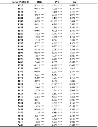
16 Tobacco 1 9 463 5 131 4,690 9 463 4,690

17 Textile 5 119 40,469 5 229 116,397 32 2,097 31,477 18 Wearing apparel 5 309 30,318 5 244 493,637 100 9,712 167,569 19 Leather and shoes 2 87 13,490 5 229 93,673 42 3,436 47,615

22 Publishing 1 4 3,696 5 123 3,647 4 316 3,647

24 Chemicals 3 153 22,856 5 212 105,746 57 2,508 35,987 35 Other transport 2 33 8,650 5 195 33,547 18 1,226 17,707 36 Furniture and other 3 44 16,316 5 216 53,841 25 1,681 28,964

40 1,473 165,737 5 202 1,229,812 42 2,816 42,436

Note.The table reports several descriptive statistics of the sample, for each 2-digit sector. A variety is defined as a product (according to the 8-digit classification) imported from a given country. All sectoral references are based on the NACE classification. S ource. Authors' calculations based on the dataset described in Section 3.1.

Table 1. Summary statistics.

S ector (NACE-2)

No. of 4-digit sectors

No. of products

(g)

No. of varieties

(z)

No. of observ. (M,z,t)

No. of products

per eq. No. of varieties

per eq. No. of observ. per eq.

Total

what follows, we denote the good imported under product labelg from countryX as a variety

z= (g; X). As such, in our analysis a variety can be seen as the basic unit of importer choice.14

In our analysis, all varieties belonging to undi¤erentiated products are dropped, as building

a quality index based on such varieties would make little sense; furthermore, since our theory

concerns consumers, we keep only varieties belonging to consumer-good intensive categories. The

varieties are selected using Rauch’s (1999) di¤erentiated products classi…cation on the one hand,

and the Eurostat’s Main Industrial Groupings on the other.15 Table 1 gives an overview of the

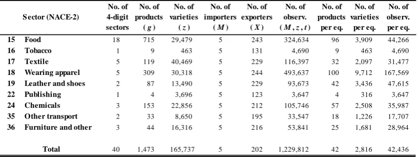
database at a 2-digit level. Overall, the database contains 40 four-digit sectors. On average,

per equation, we have 42 products g, nearly three thousands varieties z and more than forty

thousands observations(z; t). The coverage of the database varies signi…cantly across the 2-digit sectors. For example, the wearing apparel sector has on average almost ten thousands varieties

per equation, while the publishing sector has just over three hundreds.16

1 4_{Note that horizontal di¤erentiation, as discussed in the previous section, occurs at the product level. As a} result, every varietyzincludes each di¤erentiated goodsj, belonging to labelg, produced in source countryX.

1 5_{Since considering only consumer-good intensive varieties signi…cantly reduces the size of the database, for} robustness we also perform our empirical analysis using all di¤erentiated varieties, regardless their end-use catego-rization. The results hold qualitatively intact. We report the relevant …ndings in the Online Appendix, available at http://sites.google.com/site/vincenzomerella/research/…les/OnlineAppendixDRCHQG.pdf.

(12)

di-In order to guarantee a certain homogeneity in the demand function for the di¤erentiated

products, we estimate a separate demand function for each NACE 4-digit sector.17 _{Due to data}

availability, the number of separate equations we can actually estimate reduces from 40 to 39.

Taking all the speci…cs of our database into consideration, we can rewrite (9) as:

lnsz;t lns0;t= z+ t+ M + y pz;t+ lnnsz;t+ z;t (10)

This is the equation that we estimate separately for each NACE 4-digit sector. In each destination

country, sz;t measures the market share of variety z relative to total consumption of goods in

the relevant 4-digit sector, in turn computed as the sum of domestic production and imports,

minus exports. The market share is calculated in quantitative terms. We also consider an outside

variety, required by the demand system, as the domestic substitute for imports in each country,

whose market share,s0;t, is calculated as one minus the sectoral overall import penetration.18

In equation (10), we estimate quality — the term M_X in (9)— as the sum of …ve components: (i) the time invariant component ( _z), captured by variety …xed e¤ect; (ii) the common trend component ( _t), captured by year …xed e¤ect; (iii) the destination market component, captured by importer dummy ( _M); (iv) an unobserved component ( _z;t), captured by the estimation error term; and (v) the income e¤ect component, _y lnyM, obtained by introducing the log

of importer per-capita GDP as a regressor in (10). The parameter is the central object of

interest of our analysis. In equation (10), this parameter governs how a market share relate to

product quality. Since our model predicts that product quality increases with importer income,

we expect >0.

The demand function (10) allows for di¤erent degrees of substitutability across products. In

fact, in a nested logit speci…cation of demand, di¤erent substitutability patterns may arise among

groups of varieties or ‘nests’, which must however be determinedex-ante. We let product labelsg

serve as nests. In particular, it is assumed that varieties within the same product exhibit a higher

mension. This fact does not however represent an issue since, as we discuss below, each sector is by construction independently considered.

1 7_{Each 4-digit NACE sector is linked to the relevant CN 8-digit classi…cation through appropriate} correspon-dence tables provided by Eurostat.

(13)

degree of substitutability than varieties of di¤erent products. For example, a Vietnamese cotton

shirt is assumed to be a closer substitute to a Chinese cotton shirt than a Chinese nylon shirt.19

The nest termnsz;tis calculated as the import share of varietyzin the total imports of product

g(the nest), and is introduced to limit the extent of the issues arising from the independence of

irrelevant alternatives in traditional logit models.20

The substitution parameter can be interpreted as follows. If approached one, there would

be perfect substitution among varieties within the nest (e.g., between Chinese and Vietnamese cotton shirts), but no substitution across nests (e.g., no substitution between cotton and nylon shirts). As a result, if the price of a given variety increased, importers would substitute it with

varieties from the same nest but not from other nests. On the one hand, this would imply that

the varieties’relative market share would change within the nest, but not outside the nest, and

thus changes in the overall market sharesz;t would be exclusively determined by the sharensz;t

within the nest.21 In fact, in the case of an increase in its relative price, a variety easier to

substitute would have a stronger decline in its market share, even if no change occurred in its

relative quality. On the other hand, market shares of varieties in a given nest would not be

in‡uenced by price variations occurring to varieties in other nests. Of course, if approached

zero, then the opposite would occur.

Given that the price pz;t and the nest share nsz;t are endogenous, i.e., contemporaneously

correlated with the residual _z;t, in order to obtain consistent estimates of (10) we consider a number of instruments. For the unit values, pz;t, we use two sets of instruments. Given that

the COMEXT database contains neither variety-level transportation costs nor non-rival variety

characteristics (which are widely used instruments in the literature since Hausman, 1997), our

…rst set of instruments relies on non-variety speci…c data, and in particular on country level data, namely the bilateral exchange rate and a proxy for transportation costs calculated as the

1 9_{In this example, cotton shirts and nylon shirts are two distinct nests.}

2 0_{Theoretically,}_nsz;t_{should be calculated as a market share in consumption. However, given that we have no} information on the size of the domestic market at the product level, we calculate it as an import share,i.e., as the share of varietyz import in the total imports of productg. This is equivalent to the assumption that each product market in a given sector exhibits the same import penetration.

2 1_{In the example introduced above, if the price of the Chinese cotton shirt went up, importers would substitute} it with Vietnamese cotton shirts and not by Chinese nylon shirts. The overall market share of both cotton and nylon shirts would remain unchanged, while the market share of Chinese cotton shirt within the apparelsector

(14)

interaction of bilateral country distances and the oil price.22 _{This set of instruments has the}

advantage of being available for the whole sample. The second set of instruments is variety-speci…c, and consists of the average unit values of each variety observed on alternative EU markets. The idea behind using these so called Hausman instruments is that changes in unit

values in third markets can be assumed to re‡ect cost shocks and thus be used as instruments for

prices with regard to the EU member state market under consideration.23 _{The nest share,}_ns z;t,

is instrumented with the number of varieties within the nest and with the number of varieties

exported by the source country.

In what follows, we compare the results obtained using three methods: the ordinary least

square estimation (labelled ‘OLS’), which does not deal with endogeneity issues; and two

instru-mental variable estimations, one making use of the subset of non-variety-speci…c instruments only

(‘IV1’); and the other using the full set of variety and non-variety speci…c instruments (‘IV2’).

3.2 Estimation results

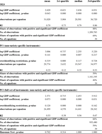
To give an overview of the goodness of the regressions, Table 2 reports a summary of the

esti-mation results, focusing on the coe¢ cient of our variable of interest, i.e., the log of per capita GDP (hereafter, GDP coe¢ cient).24 Given the relatively large number of separate equations,

one per 4-digit sector, the table shows the distribution of the coe¢ cients and of the associated

p-values across our estimations.25 _{From top to bottom, the three boxes in Table 2 illustrate the}

results of the OLS estimation and of the two sets of IV estimations, the …rst one considering

only non-variety speci…c instruments (IV1), and the second one with the full set of instruments

(IV2). Hereafter, we refer to the IV2 approach as the benchmark estimation, since it deals with

endogeneity using a wider set of instruments, thereby providing more e¢ cient estimates.

As expected, the mean of the GDP coe¢ cient is positive in all di¤erent estimation strategies,

suggesting that richer countries’consumers tend to import higher quality goods from their trade

2 2_{Bilateral exchange rates are taken from IFS database; distances are from the CEPII database.}

2 3_{We use average unit values in order to minimize the e¤ect of parallel trade potentially in place among the} EU members, which could a¤ect the variety market share as well as its price. Since the largest economies in the EU are those included in our dataset, averaging across alternative declarants has the advantage of obtaining the instrument for virtually every variety in the sample. As we show in the next subsection, our tests are suggestive of the validity and reliability of the instrument.

(15)

OLS

log GDP coefficient 2.620 -0.621 2.636 6.031 log GDP coefficient, p-value 0.043 0.000 0.000 0.000

observations per equation 31,020 5,904 20,501 36,720

R2 0.79 0.73 0.79 0.86

No. of observations 1,209,783

69%

No. of equations 39

overidentifying restrictions, p-value 0.319 0.000 0.117 0.728 observations per equation 29,774 5,632 19,547 34,977

R2 0.33 0.12 0.32 0.53

46%

overidentifying restrictions, p-value 0.120 0.000 0.000 0.162

R2 0.53 0.38 0.56 0.67

66%

No. of observations 955,480

59%

Hausman Test , p-value 0.702 0.314 1.000 1.000 59% S hare of equations with positive and significant GDP coefficient

S hare of observations with positive and significant GDP coefficient

IV1 (non-variety specific instruments)

88%

Table 2. Summary of benchmark estimation results: coefficients of log GDP.

mean 1st quartile median 3rd quartile

Note.The table reports several moments of the distribution of the estimates of the log of importer's per capita GDP coefficients, based on a separate demand function for each NACE 4-digit sector. The dependent variable is the log of the variety market share in a given sector. A variety is defined as a product (according to the NACE 8-digit classification) imported from a given country. The variety unit value and a nest term (computed as the variety import share for a given product) are included as regressors, along with other determinants of quality, namely: variety, year and importer effects. The component of quality measure unrelated to income is estimated as the sum of these three effects plus the error term. Each panel of the table refers to a different set of regressions: the top panel summarizes the results obtained using the ordinary least square (OLS) estimator; the mid panel those obtained with an instrumental variable estimator using a subset of non-variety specific instruments only (IV1); the bottom panel those obtained with an instrumental variable estimator using the full set of variety and non-variety specific instruments (IV2). The Hansen-Sargan test is used to assess the over-identifying restrictions. The Hausman test assesses the validity of the full set of instruments. S ource.Authors' calculations based on the dataset described in Section 3.1.

IV2 (full set of instruments: non-variety and variety specific instruments)

S hare of equations with positive and significant GDP coefficient S hare of observations with positive and significant GDP coefficient

S hare of equations with positive and significant GDP coefficient

(16)

OLS IV1 IV2

2.620 3.006 2.371

p-value 0.021 0.006 0.028

no. of observations 39 39 39

mean of log GDP coefficient

Note.M ean test conducted by regressing the log GDP coefficients (originating from the set of estimates summarized in Tables 2 and 6) on a constant, assuming a heteroscedastic distribution of the coefficients. S ource. Authors' calculations based on the dataset described in Section 3.1.

Table 3. Mean test for log GDP coefficients.

partners. The result of our estimations is not driven by just a few sectors: across the 39 estimated

equations, the share of positive and statistically signi…cant GDP coe¢ cients is 59%, and involves

66% of the nearly one million observations in our sample. Table 2 also reports the distribution of

the p-values associated to the GDP coe¢ cient estimates. These …gures represent the measure of

statistical signi…cance for single equations. To assess the joint signi…cance of our GDP coe¢ cients

we need to run a formal test, whose results are shown in Table 3, separately for each approach.

It is straightforward to notice that all our estimates are signi…cantly di¤erent from zero. All

statistical exercises thus lend support to our prediction that product quality rises with importer

income.

We also conducted a number of exercises to assess the robustness of our results. The …rst

one determines to what extent the Linder hypothesis may bias the quality estimates and, hence,

might distort the relationship between quality and income. The Linder hypothesis postulates

that countries with similar per capita GDP, displaying similar demand structures, would trade

more with each other. In this perspective, any destination country would exhibit an inverse

relationship between the market shares captured by exporters from a particular source country

and the per capita GDP gap between the two countries. To check whether our results might be

mainly driven by this occurrence, we perform again our estimation exercise including as an

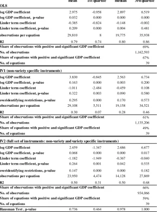
addi-tional regressor a ‘Linder term’, computed as the absolute value of the di¤erence between the log

of per capita GDPs of the relevant importer and exporter. Table 4 reports the results relative to

the GDP coe¢ cients and the Linder terms.26 _{As expected, the Linder term is negative (though,}

on average, not statistically signi…cant), but its introduction seems to have little in‡uence on

(17)

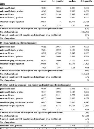
OLS

log GDP coefficient 2.975 -0.958 2.897 6.519

log GDP coefficient, p-value 0.032 0.000 0.000 0.000

Linder term coefficient -0.385 -0.824 -0.148 -0.002

Linder term coefficient, p-value 0.209 0.000 0.004 0.481

observations per equation 29,810 8 19,775 35,938

R2 0.79 0.74 0.80 0.86

69%

67%

Linder term coefficient -1.011 -2.484 -0.459 0.108

R2 0.30 0.07 0.28 0.46

61%

49%

Linder term coefficient -1.182 -1.949 -0.367 -0.040

R2 0.50 0.31 0.50 0.68

66%

59%

Hausman Test , p-value 0.736 0.464 0.978 1.000

Note.The table reports several moments of the distribution of the estimates of the coefficients of the log of importer's per capita GDP and of a Linder term (computed as the absolute value of the difference in per capita GDP between importer and exporter), based on a separate demand function for each NACE 4-digit sector. The dependent variable is the log of the variety market share in a given sector. A variety is defined as a product (according to the NACE 8-digit classification) imported from a given country. The variety unit value and a nest term (computed as the variety import share for a given product), are included as regressors, along with other determinants of quality, namely: variety, year and importer effects. The component of quality measure unrelated to income is estimated as the sum of these three effects plus the error term. Each panel of the table refers to a different set of regressions: the top panel summarizes the results obtained using the ordinary least square (OLS) estimator; the mid panel those obtained with an instrumental variable estimator using a subset of non-variety specific instruments only (IV1); the bottom panel those obtained with an instrumental variable estimator using the full set of variety and non-variety specific instruments (IV2). The Hansen-Sargan test is used to assess the over-identifying restrictions. The Hausman test assesses the validity of the full set of instruments. S ource.Authors' calculations based on the dataset described in Section 3.1.

IV2 (full set of instruments: non-variety and variety specific instruments) S hare of equations with positive and significant GDP coefficient

Table 4. Summary of estimation results: coefficients of log GDP and Linder term.

(18)

OLS IV1 IV2

1.062 0.228 0.830

p-value 0.038 0.007 0.013

-10.944 -2.673 -8.837

p-value 0.039 0.007 0.011

no. of observations 1,209,784 1,161,196 955,481 mean of log GDP coefficient

constant

Note.The table reports the OLS estimates of the coefficients of the log of importer's per capita GDP and of a constant. The dependent variable is a measure of product quality that abstracts from the income component, and is computed as the sum of variety, year and importer effects plus the error term; the results of the set of regressions from which these effects originate are summarized in Table 9. Each column of the table refers to a different regression: the left column summarizes the results obtained using the ordinary least square (OLS) estimator; the mid column those obtained with an instrumental variable estimator using a subset of non-variety specific instruments only (IV1); the right column those obtained with an instrumental variable estimator using the set of variety and non-variety specific instruments (IV2). S ource.Authors' calculations based on the dataset described in Section 3.1.

Table 5. Regressions of quality measures on importer's log GDP.

the GDP coe¢ cients, which remain positive and signi…cant, and actually exhibit a slight rise in

their average magnitudes relative to those delivered by our benchmark exercises.

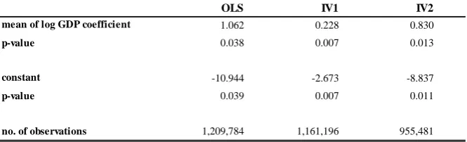
As a further robustness exercise, we test the relationship between quality and income

follow-ing a two stage approach. First, we estimate product quality without considerfollow-ing the income

term _y in (10), in line with the original Khandelwal (2010) speci…cation. Then, we assess the relationship between quality estimates and importer income by means of a OLS regression. Table

5 summarizes the results that we obtain on aggregate.27 Once again, these results show that

the relationship between product quality and importer’s income per capita is positive and highly

signi…cant.

3.3 Discussion

In our estimations, the GDP coe¢ cient captures how our quality measure changes with the log

of the importer’s per capita income. As such, we can interpret its magnitude in terms of

semi-elasticity: that is, a ten percent increase in importer income produces, on average, approximately

a0:23units rise in product quality.28

2 7_{Tables 9 and 10 in Appendix B respectively report the price and nest coe¢ cients of the …rst-stage estimation} and the results relative to the coe¢ cients of log GDP at the sectoral level of the second-stage estimation.

(19)

Of course, our main interest is actually in whether the estimated magnitude of the GDP

coe¢ cient should be considered as sizeable or negligible. As it is often the case with

semi-elasticity, pinpointing a benchmark against which to compare the …gure would help in obtaining

a more transparent assessment. Furthermore, our …gure refers to the average of the income

semi-elasticities of quality across heterogeneous sectors. In order to get a more reliable assessment, the

benchmark should then be determined at the sectoral level, and the average should be computed

on the sectoral …gures ‘standardized’against the relevant benchmarks.

We identify the benchmark as the length of the sectoral quality ladder. A quality ladder is

de…ned as the set of available (or, in this case, observed) qualities in a given market (here, the

relevant sector). Its length is measured by the di¤erence between the highest and the lowest

quality levels. Divided by the length of the quality ladder, a (properly scaled down as above)

sectoral GDP coe¢ cient is interpretable as the percentage distance covered by moving from

consuming a product to another across the sectoral quality ladder, in response to a given

per-centage increase in importer income. The resulting sectoral …gures are ‘adimensional’statistics,

hence their mean produces a fairly transparent and reliable indicator of imports’average product

quality upgrading as importer income rises.

The newly developed quality upgrading indicator reveals that a ten percent increases in

importer income produces a shift of the products consumed across the quality ladders that

covers, on average, 2:75% of their length. This implies that an importer that is twice as rich as another enjoys products sitting, on average, in a position20% higher in the sectoral quality ladders; and that in order for the shift in the product consumed to cover 50% of the quality ladder, an importer should be 5:6 times as rich. Thanks to the quality upgrading indicator, we may also deduce more concrete …gures. For example, we can infer that the 2013 per capita

income distribution interdecile ratio produces a shift in the products imported that covers an

average distance across the sectoral qualities ladders of about56%in France and Germany;71%

in Italy;74%in Spain; and68%in the UK. If we dared bringing our quality upgrading indicator out of sample, the average distance covered across the sectoral quality ladders would be ranging

from less than50%in Iceland and Denmark to well over80%in the United States and Chile.29 formal discussion on how we derive this …gure, together with the rest of the auxiliary computations used in this subsection, see Appendix A.3.

(20)

Another noteworthy aspect arising from our estimates is that the magnitude of the GDP

coe¢ cients is rather varied across sectors. This might be partly due to the fact that, at a 4-digit

disaggregation level, products are quite heterogeneous in some sectors; and partly to the mere

fact that the dataset is admittedly somewhat noisy. To put things into perspective, we may focus

our attention to those sectors where products are relatively ‘homogeneous’(i.e., cross-products substitutability is estimated to be relatively high), and demand is ‘well-behaved’(i.e., negatively related to the product price): that is, sectors where the nest share coe¢ cient, , is estimated

to be positive; the price coe¢ cient, , negative; and both coe¢ cients statistically signi…cant.

The share of sectors with positive and signi…cant GDP coe¢ cients raises from59%to70%when ‘homogeneous’ sectors are considered, and up to 83% if we also condition on ‘well-behaved’ demand.

A further possible reason for the observed heterogeneous magnitude of the GDP coe¢ cients

may arise from the sectoral di¤erences in thescopefor quality upgrading. For example, if higher quality products are relatively inexpensive in a given sector, then there could be more scope

for purchasing them even with a limited rise in the importer income, and vice versa. We may

think of the length of a sectoral quality ladder also as an observed measure of the scope for quality upgrading, since by de…nition it reveals the largest possible quality range for a given

income di¤erential: the one between the richest and the poorer importer.30 _{In this context, one}

could expect GDP coe¢ cients to be larger in those sectors exhibiting longer quality ladders. For

the generality of sectors, the correlation between the two variables is however not statistically

signi…cant ( 0:19with p-value0:24). If we condition on ‘homogeneous’and ‘well-behaved’sectors (in the sense speci…ed above), then the correlation becomes positive and signi…cant (0:75 with p-value0:005) as expected.

Finally, a note on potentially interesting further development and investigation of the link

between product quality and importer income within the framework used in this paper. The

theory presented here relies on the assumption that some products are imported because, though

11:4in Italy,12:7in Spain,10:6in the UK; and5in Iceland,5:3in Denmark,18:5in the United State,20:6in Chile (source: OECD).

(21)

ine¢ ciently produced, they meet the idiosyncratic taste of some consumers. Such products are

therefore expensive and capture small markets shares, thus are accordingly assigned a low quality

level. In the presence of a bell-shaped income distribution in the destination country, however,

our empirical results on the link between import quality and importer income are suggestive of

a competing explanation for niche products. Although e¢ ciently produced, some top quality

products might be so expensive to be a¤ordable only for a thin fraction of rich importers. These

products are also assigned a low quality level though, since they command high prices and

small (quantitative) market shares. Unfortunately, we are at present unable to disentangle

the two groups of products, since the available data include neither end user characteristics

of the importer, nor su¢ cient elements to determine whether the exported goods are e¢ ciently

produced.

It should be noted, however, that this caveat should not substantially a¤ect our …ndings.

Fail-ure to identify the quality level of high segment products would in fact shorten the quality ladder,

if anything underestimating the scope for quality upgrading. In this perspective, the estimated

GDP coe¢ cients might actually be interpreted as a lower bound to the magnitude of the actual

link between product quality and importer income. Furthermore, it should be noted that the

quality upgrading indicator developed above would be in‡uenced by the identi…cation issue both

at thenumerator(downward-biased GDP coe¢ cient) and at thedenominator (downward-biased quality ladder length). Under the assumption that the two biases are not too disproportionate,

one may conjecture that this indicator might provide not only a more transparent …gure, but

also a more reliable measure of the relationship between import quality and importer income

than our estimated GDP coe¢ cients, even at the sectoral level.

4 Conclusion

This paper provides theoretical support and empirical evidence to one of the major issues in

the international trade literature: whether quality of imports rises systematically with importer

income. Our framework builds on the discrete choice models approach. The novelty of the

paper lies in the joint consideration of two results stemming from our framework. First, product

(22)

measure depend not only on product prices but also on market shares; hence, in our estimations,

we depart from the traditional assumption that prices are proxies for quality.

We test our hypothesis on a dataset consisting of import data of …ve EU countries (namely:

France, Germany, Italy, Spain and the UK), and over a 13-year time span,i.e., 1995-2007. The main contribution of the paper is that we …nd a positive and signi…cant relationship between the

per capita GDP of the selected countries and the alternative quality measure delivered by the

model. Our estimates are robust to a number of controls and to three di¤erent methodological

approaches, based on di¤erent instrumental variable strategies.

As an additional contribution, we derive from our estimates a novel, fairly transparent and,

under certain assumptions, reliable indicator of import quality upgrading as importer income

rises. Based on this indicator, our …ndings reveal that doubling importer income brings about an

average product quality upgrading of20%, relative to the length of the quality ladders. Looking at the 2013 per capita incomes in our …ve destination countries, this in turn implies that moving

up from the …rst to the ninth decile of the income distribution generates a ‘in-sample’product

quality upgrading of about65%the length of the quality ladders; out-of-sample, that percentage goes up to almost90%in other OECD countries.

Appendices

A

Proof of theoretical results

A.1 Derivation of aggregate demand (2)

Consider the choice of a generic good(j; X)over all possible alternatives in the market, namely f(k; Y)_g, with k₆= j whenY =X. Given (1), the decision rule for consumer i in country M

is as follows: consume good (j; X)only if V_j;Xi;M > V_k;Yi;M,₈(k; Y)₆= (j; X). Our task is thus to compute the probability:

Pr (j; X_ji; M) = Pr "i;M_j;X > max

Y=fN;S;Mg maxk

n

M k;Y +"

i;M k;Y

M j;X

o

(k;Y)6=(j;X)

(23)

The term on the right-hand side represents the joint probability that horizontal di¤erentiation

of good(j; X)is valued by consumeriin countryM more than that of any other good. We can therefore write:

Pr (j; X_ji; M) =

Z +1 1

f "i;M_j;X exp

Z

k6=j

ln

Z "i;M_j;X+ M j;X Mk;X

1

f "i;M_k;X d"i;M_k;X

!

dk

+ X

Y6=X

Z 1 0

ln

Z "i;Mj;X+ M j;X

M k;Y

1

f "i;M_k;Y d"i;M_k;Y

!

dk

1

Ad"i;M_j;X (11)

where, exploiting the properties of the exponential function, we have expressed the product of a

generic sequencezh as:

Y

h

zh=Y

h

exp (ln (zh)) = expX

h

(ln (zh))

The term R" i;M j;X+

M j;X Mk;Y

1 f "

i;M k;Y d"

i;M

k;Y is the cumulative distribution function (CDF) of "i;M_k;Y up to the value"i;M_j;X + M_j;X M_k;Y. Since"i;M_k;Y is a Gumbel random variable, we have:

Z "i;M_j;X+ M j;X Mk;Y

1

f "i;M_k;Y d"i;M_k;Y = Pr "i;M_k;Y < "i;M_j;X + M_j;X M_k;Y = exp exp h"i;M_j;X + M_j;X M_k;Yi

Replacing this value into (11) yields:

Pr (j; X_ji; M) =

Z +1 1

f "i;M_j;X exp

Z

k6=j

exp h"i;M_j;X + M_j;X M_k;Xi dk

X

Y6=X

Z 1 0

exp h"i;M_j;X + M_j;X M_k;Yi dk

1

Ad"i;M_j;X (12)

Also, the probability density function (PDF) of a Gumbel random variable is:

(24)

Plugging this expression into (12), and rearranging, we obtain:

Pr (j; X_ji; M) =

Z +1 1

exp "i;M_j;X exp "i;M_j;X 1 +

Z

k6=j

exp M_k;X M_j;X dk

+ X

Y6=X

Z 1 0

exp M_k;Y M_j;X dk d"i;M_j;X

=

Z +1 1

exp "i;M_j;X exp "i;M_j;X

X

Y=fN;S;Mg

Z 1 0

exp M_k;Y M_j;X dk d"i;M_j;X (13) where in the last equation we have exploited the fact that1 = exp (0) = exp M_j;X M_j;X .

Denote:

$ X

Y=fN;S;Mg

Z 1 0

exp M_k;Y M_j;X dk

and:

g "i;M_j;X exp "i;M_j;X $exp "i;M_j;X

Note thatg "i;M_j;X is the PDF of a Gumbel random variable with CDF:

exp $exp "i;M_j;X =$

since:

dexp $exp "i;M_j;X =$

d" =

exp $exp "i;M_j;X

$ $exp "

i;M j;X

= exp "i;M_j;X $exp "i;M_j;X =g "i;M_j;X

Thus, we can use the last equation to rewrite (13) as:

Pr (j; X_ji; M) = _P 1

Y=fN;S;Mg

R1

0 exp

M

k;Y Mj;X dk

2 4exp

0

@ exp "i;M_j;X X Y=fN;S;Mg

Z 1 0

exp M_k;Y M_j;X dk

1 A 3 5

+1

(25)

where the term in square brackets vanishes since its limit value for"i;M_j;X _!+₁equals one, and for"i;M_j;X _{! 1}equals zero. Finally, we multiply and divide byexp M_j;X to get:

Pr (j; X_ji; M) =

exp M_j;X

P

Y=fN;S;Mg

R1

0 exp

M k;Y dj

Noting that countryM has measure M, integrating over consumers, (2) obtains.

A.2 Derivation of optimality conditions (4) and (5)

Di¤erentiating (3) with respect top, and setting the resulting expression equal to zero, yields:

1 pM_j;X wX q

2

2AX

Mexp Mq pMj;X

P

Y=fM;N;Sg

R1

0 exp

M k;Y dk

= 0

simplifying and rearranging, (4) straightforwardly obtains. Di¤erentiating (3) with respect toq,

and setting the resulting expression equal to zero, we get:

"

q_j;XM AX +

M

p wX q

M j;X 2 2AX !# Mexp M qM j;X p P

Y=fM;N;Sg

R1

0 exp

M k;Y dk

= 0

Simplifying this expression returns:

q_j;XM AX =

M

p wX q

M j;X

2

2AX

!

Using (4) to substitute forp=pM

j;X, simplifying and rearranging leads immediately to (5).

For completeness, we might also compute the (average) valuation of good (j; X)in countryM. Plugging (4) into the de…nition of Mj;X, we have:

M

j;X =qMj;X M

2AXq M

(26)

Then, using (5) to substitute forqM

j;X, and rearranging we get:

M j;X =

M 2 AX

2 1 wX (14)

We may note that all …rms within each source country optimally supply to country M goods

that are, on average, equally valued ( M_j;X = M_X,₈j). Furthermore, by comparing (14) computed for the two countries, it follows that and goods from N are given larger valuation than those

fromS if

M 2₍_A

N AS)

2 > (wN wS) (15)

since either consumers’valuation for quality must be su¢ ciently high, or technological capabilities

inN su¢ ciently superior, to overcome its disadvantage in manufacturing costs.

A.3 Auxiliary derivations for Section 3.3

GDP coe¢ cients and quality ladder length. Consider a sector s with a quality space

of measure s (hereafter, quality ladder length), and suppose that the following relationship

between quality (qs) and per capita GDP (Y) holds at the sectoral level:

qs= _slnY

where _s is a …xed sectoral parameter. For a given change in per capita GDP, say from Y0 _to

Y1 _gY0_{, quality vary from}_q0

s toq1s according to the expression:

qs qs1 q0s= slnY1 slnY0= sln Y1=Y0 = slng (16)

In the text, we refer to the average value of the GDP coe¢ cient, ^_s ( _s) = 2:371, where

( )here denotes the arithmetic mean operator across sectors. By averaging both sides of (16), we obtain:

^

qs ( qs) = ^_slng

(27)

2:371 0:095 = 0:23units.

We may ‘standardize’(16) by dividing both sides by s, to get:

s qs

s

= s

s

lng= slng

where s s= s. Here, s can be interpreted as the distance covered by the quality variation

relative to the quality ladder length. We can average both sides of the last expression to obtain:

^_s= ^slng

In the data, ^s is 0:29. Hence, for a10% growth in per capita GDP (g = 1:1), the quality

ladder is on average climbed up by^_s= 0:29 0:095 = 2:75%. If per capita GDP doubles (g= 2), then ^_s = 0:29 0:69 = 20%. To cover, on average, half of the quality ladder (^_s= 50%), per capita GDP should grow by the factorg=e^s=^s ₌_e0:50=0:29_{= 5}_:₆_.

Regarding the 2013 interdecile ratios of the income distribution in the cited countries, we

obtain an average climbing up the quality ladder of about ^_s = 0:29 ln 6:9 = 56% in France,

^_s= 0:29 ln 6:8 = 55:6%in Germany,^_s= 0:29 ln 11:4 = 71%in Italy,^_s= 0:29 ln 12:7 = 74%

in Spain,^_s= 0:29 ln 10:6 = 68%in the UK;^_s= 0:29 ln 5 = 47%in Iceland,^_s= 0:29 ln 5:3 = 48% in Denmark,^_s= 0:29 ln 18:5 = 85% in the United States, and ^_s = 0:29 ln 20:6 = 88%

in Chile.

Cost of quality upgrading and quality ladder length. In order to explicitly di¤erentiate

the cost functions across sectors, let a sectoral parameter _s(where the subscriptsidenti…es the sector under consideration) enter the cost function, to obtain:

wX+ sq2

2AX

Di¤erentiating this expression with respect toqand using (5) yields the sectoral measure of the

cost of quality upgrading:

s s

(28)

Finally, de…ning the sectoral quality ladder in a given destination country M as the di¤erence

between the highest and the lowest quality levels of the goods imported byM, the model yields

L M_N M_S . Using the de…nition of M_X and once again (5), we may rewrite this expression as:

Ls L s; M = M

s M

(AN AS) = 1

s M

(AN AS)

It is then immediate to notice the inverse relationship between the length of the ladderLsand the

cost of quality upgrading s: hence, a sector characterized by a lower cost of quality upgrading

(29)

B

Additional tables

OLS

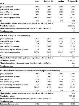
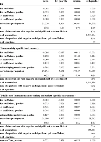
price coefficient -0.003 -0.004 0.000 0.000 price coefficient, p-value 0.058 0.000 0.000 0.001

nest coefficient 0.880 0.833 0.889 0.924

nest coefficient, p-value 0.000 0.000 0.000 0.000

R2 0.79 0.73 0.79 0.86

87%

82%

price coefficient -0.077 -0.047 -0.007 0.000 price coefficient, p-value 0.288 0.000 0.224 0.576 nest coefficient 0.245 -0.127 0.683 0.910 nest coefficient, p-value 0.110 0.000 0.004 0.106

R2 0.33 0.12 0.32 0.53

68%

44%

price coefficient -0.003 -0.007 -0.001 0.000

price coefficient, p-value 0.287 0.001 0.129 0.594

nest coefficient 0.526 0.297 0.756 0.995

nest coefficient, p-value 0.045 0.000 0.000 0.013

R2 0.53 0.38 0.56 0.67

69%

44%

Hausman Test , p-value 0.702 0.314 1.000 1.000 Note.The table reports several moments of the distribution of the estimates of the coefficients of price and nest term (computed as the variety import share for a given product), based on a separate demand function for each NACE 4-digit sector. The dependent variable is the log of the variety market share in a given sector. A variety is defined as a product (according to the NACE 8-digit classification) imported from a given country. The log of importer's per capita GDP is included as a regressor, along with other determinants of quality, namely: variety, year and importer effects. The component of quality measure unrelated to income is estimated as the sum of these three effects plus the error term. Each panel of the table refers to a different set of regressions: the top panel summarizes the results obtained using the ordinary least square (OLS) estimator; the mid panel those obtained with an instrumental variable estimator using a subset of non-variety specific instruments only (IV1); the bottom panel those obtained with an instrumental variable estimator using the full set of variety and non-variety specific instruments (IV2). The Hansen-Sargan test is used to

Table 6. Summary of benchmark estimation results: price and nest coefficients.

mean 1st quartile median 3rd quartile

S hare of observations with negative and significant price coefficient

S hare of equations with negative and significant price coefficient

S hare of observations with negative and significant price coefficient

S hare of equations with negative and significant price coefficient S hare of equations with negative and significant price coefficient

IV2 (full set of instruments: non-variety and variety specific instruments)

(30)

Sector (NACE-4)

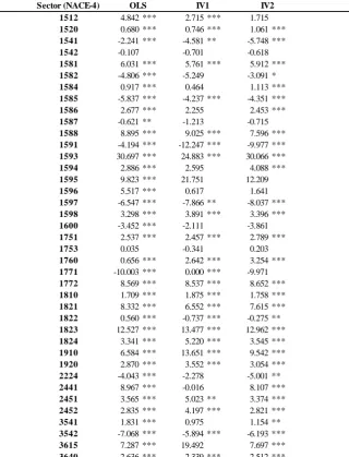
1512 4.842 *** 2.715 *** 1.715

1520 0.680 *** 0.746 *** 1.061 ***

1541 -2.241 *** -4.581 ** -5.748 ***

1542 -0.107 -0.701 -0.618

1581 6.031 *** 5.761 *** 5.912 ***

1582 -4.806 *** -5.249 -3.091 *

1584 0.917 *** 0.464 1.113 ***

1585 -5.837 *** -4.237 *** -4.351 ***

1586 2.677 *** 2.255 2.453 ***

1587 -0.621 ** -1.213 -0.715

1588 8.895 *** 9.025 *** 7.596 ***

1591 -4.194 *** -12.247 *** -9.977 ***

1593 30.697 *** 24.883 *** 30.066 ***

1594 2.886 *** 2.595 4.088 ***

1595 9.823 *** 21.751 12.209

1596 5.517 *** 0.617 1.641

1597 -6.547 *** -7.866 ** -8.037 ***

1598 3.298 *** 3.891 *** 3.396 ***

1600 -3.452 *** -2.111 -3.861

1751 2.537 *** 2.457 *** 2.789 ***

1753 0.035 -0.341 0.203

1760 0.656 *** 2.642 *** 3.254 ***

1771 -10.003 *** 0.000 *** -9.971

1772 8.569 *** 8.537 *** 8.652 ***

1810 1.709 *** 1.875 *** 1.758 ***

1821 8.332 *** 6.552 *** 7.615 ***

1822 0.560 *** -0.737 *** -0.275 **

1823 12.527 *** 13.477 *** 12.962 ***

1824 3.341 *** 5.220 *** 3.545 ***

1910 6.584 *** 13.651 *** 9.542 ***

1920 2.870 *** 3.552 *** 3.054 ***

2224 -4.043 *** -2.278 -5.001 **

2441 8.967 *** -0.016 8.107 ***

2451 3.565 *** 5.023 ** 3.374 ***

2452 2.835 *** 4.197 *** 2.821 ***

3541 1.831 *** 0.975 1.154 **

3542 -7.068 *** -5.894 *** -6.193 ***

3615 7.287 *** 19.492 7.697 ***

3640 2.636 *** 2.339 *** 2.512 ***

Table 7. Benchmark estimation results: coefficients of log GDP by 4-digit sector.

OLS IV1 IV2