Absolute density measurements in the middle atmosphere

Geophysicae

Absolute density measurements in the middle atmosphere

M. Rapp1, J. Gumbel2, and F.-J. L ¨ubken1

1_{Leibniz Institute of Atmospheric Physics, Schlossstr. 6, 18225 K¨uhlungsborn, Germany} 2_{Department of Meteorology, Stockholm University, 10691 Stockholm, Sweden}

Received: 6 October 2000 – Revised: 21 February 2001 – Accepted: 3 April 2001

Abstract. In the last ten years a total of 25 sounding rock-ets employing ionization gauges have been launched at high latitudes (∼70◦N) to measure total atmospheric density and its small scale fluctuations in an altitude range between 70 and 110 km. While the determination of small scale fluc-tuations is unambiguous, the total density analysis has been complicated in the past by aerodynamical disturbances lead-ing to densities inside the sensor which are enhanced com-pared to atmospheric values. Here, we present the results of both Monte Carlo simulations and wind tunnel measure-ments to quantify this aerodynamical effect. The comparison of the resulting ‘ram-factor’ profiles with empirically deter-mined density ratios of ionization gauge measurements and falling sphere measurements provides excellent agreement. This demonstrates both the need, but also the possibility, to correct aerodynamical influences on measurements from sounding rockets.

We have determined a total of 20 density profiles of the mesosphere-lower-thermosphere (MLT) region. Grouping these profiles according to season, a listing of mean density profiles is included in the paper. A comparison with density profiles taken from the reference atmospheres CIRA86 and MSIS90 results in differences of up to 40%. This reflects that current reference atmospheres are a significant potential error source for the determination of mixing ratios of, for ex-ample, trace gas constituents in the MLT region.

Key words. Middle atmosphere (composition and chem-istry; pressure, density, and temperature; instruments and techniques)

1 Introduction

During the last ten years a total of 25 sounding rockets have been launched by the Atmospheric Physics group of Bonn University (which is now at the Leibniz Institute of Atmo-spheric Physics in K¨uhlungsborn) carrying ionization gauges

Correspondence to: M. Rapp (rapp@iap-kborn.de)

to measure the neutral number density and its small scale fluctuations in an altitude range between 70 and 110 km. For a compilation of dates, flight labels, etc., see Table 1. The fluctuations have been used to unambiguously deduce turbu-lent parameters, such as the turbuturbu-lent energy dissipation rate (L¨ubken, 1992, 1997). On the other hand, the derivation of absolute number densities is complicated by the fact that at-mospheric densities are disturbed by the supersonic motion of the rocket vehicle, leading to densities inside the sensor, which are significantly larger than atmospheric densities.

In this paper we describe a procedure to quantify this aero-dynamic effect, both experimentally and numerically. We first give a short description of the ionization gauges and characterize the aerodynamic problem in more detail. We then present the results of wind tunnel measurements of the so-called ‘ram factor’, i.e. the ratio between the density ac-tually measured by the gauge and the undisturbed density of the flow. We use these results and the numerical results of Monte Carlo simulations of the density fields inside the gauges to determine altitude profiles of the ram-factors in or-der to correct the measured densities. Finally, we use the cor-rected density measurements to deduce mean density profiles for selected times of the year (January until March, July until August, and September until October). These mean profiles are compared to profiles from reference atmospheres like CIRA86 (Fleming et al., 1990) and MSIS90 (Hedin, 1991).

2 Experimental technique

Table 1. Listing of all TOTAL and CONE flights. In the last column the gauge type is indicated: T: TOTAL, C: CONE

Flight Date Time (UT) apogee gauge [km]

DAT13 22/01/90 10:20:00 132 T DAT50 25/02/90 19:20:00 128 T DAT62 06/03/90 02:41:00 133 T DAT73 08/03/90 22:53:00 119 T DAT76 09/03/90 00:25:00 130 T DAT84 11/03/90 20:42:00 131 T DBN01 20/02/90 04:54:00 128 T DBN02 06/03/90 05:18:28 128 T DBN03 13/03/90 04:21:00 128 T TURBO-B 01/08/91 01:40:00 131 T TURBO-A 09/08/91 23:15:00 130 T LT01 17/09/91 23:43:00 124 T LT06 20/09/91 20:48:00 129 T LT13 30/09/91 20:55:15 130 T LT17 03/10/91 22:27:30 129 T LT21 04/10/91 00:08:00 131 T SCT03 28/07/93 22:23:00 128 C SCT06 31/07/93 01:46:00 127 C ECT02 28/07/94 22:39:00 124 C ECT07 31/07/94 00:50:33 126 C ECT12 12/08/94 00:53:00 129 C NLTE-1 03/03/98 22:33:00 133 C MDMI05 06/07/99 00:06:00 102 C MSMI03 06/05/00 17:08:00 106 C MSMI05 15/05/00 00:46:00 102 C

absolute densities, the gauges are calibrated in the labora-tory using a high quality pressure sensor, such as a Baratron. A schematic presentation of the gauges TOTAL and CONE is shown in Fig. 1. As is seen from this figure, the main difference between the two ionization gauges is their geo-metrical design. TOTAL is a ‘closed’ gauge, where the tri-ode system is placed inside a cylindrical tube accessible only by ambient molecules through a small orifice (Hillert et al., 1994). Atmospheric air molecules can enter the ionization volume only after at least two collisions with the tube walls. In contrast, CONE consists of spherical electrode grids of high transparency without being surrounded by any struc-ture (Giebeler et al., 1993). This allows the air molecules to stream ‘through’ the sensor. The main purpose of the CONE design is to reduce the instrumental time constant, thus enhancing the ability to resolve turbulent fluctuations of even smaller scales than was possible with TOTAL. Note that CONE posseses two more electrodes than TOTAL. While the outermost grid is biased to+6V to measure electrons, the next-inner grid (−15V) is meant to shield the ionization gauge from ambient plasma.

Both ionization gauges took data at a frequency of∼3 kHz, resulting in a theoretical altitude resolution of∼0.3 m for a typical rocket velocity of 1000 m/s. However, due to the spin modulation, the data must be averaged, resulting in an ef-fective altitude resolution of∼200 m for the total number

Structure Shielding grid

Inflow Inflow

Entrance grid Baffle

Anode Ion collecor

Filament Accomodation

chamber

Shielding grid Electron collector

Fig. 1. Sketches of the ionization gauges TOTAL (left) and CONE (right). For more technical details on the gauges (dimensions, volt-ages, etc.), see the papers by Hillert et al. (1994) and Giebeler et al. (1993).

density measurement.

3 Aerodynamic effects

While the procedure to derive absolute number densities from the ionization gauge current works well in the laboratory where the gas streams slowly into the measuring volume, the densities are modified if the gauge is mounted on a sound-ing rocket. These rockets typically move at a speed of sev-eral times the speed of sound. Compression waves develop in the front of such payloads, leading to a disturbed density and temperature field around the vehicle. Thus, the density measured by CONE or TOTAL is enhanced relative to the ambient density by a ram-factor fram:

nmeas=fram·n (1)

wherenmeas is the density measured by the instrument and

nis the undisturbed atmospheric density. For a general dis-cussion of the influence of aerodynamics on rocket-borne in situ measurements in the middle atmosphere, we refer to Bird (1988) and Gumbel (2001b).

How can this ram-factor be determined? It turns out that it is very difficult to access this factor theoretically: the atmo-spheric altitude range of interest (110–70 km) includes the altitude region where the mean free path of the air molecules is of similar magnitude as typical dimensions of the gauges (some centimeters). Flow characteristics are usually de-scribed by means of the Knudsen numberKn=λ/L, where

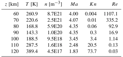
Table 2. Atmospheric and aerodynamic parameters during a sound-ing rocket flight in summer for an apogee of 130 km. Atmospheric temperatures and densities have been adopted from CIRA86 for the month July and 70◦N (Fleming et al., 1990). zdenotes altitude, T temperature,nnumber density,Mathe Mach number,Knthe Knudsen number, andRethe Reynolds number. KnandRehave been calculated forL=5 cm.

z[km] T [K] n[m−3] Ma Kn Re 60 260.9 8.7E21 4.00 0.004 1107.1 70 220.6 2.5E21 4.07 0.01 335.2 80 168.8 5.9E20 4.35 0.06 92.9 90 143.3 1.0E20 4.35 0.3 16.9 100 188.5 9.5E18 3.45 3.4 1.14 110 287.5 1.6E18 2.48 20.5 0.13 120 389.4 4.5E17 1.83 73.7 0.03

Table 3. Parameters of the wind tunnel experiments. z˜ denotes the altitude which corresponds to the density in the experiment chamber. The altitude dependence of density has been taken from CIRA86 for the month July and a geographical latitude of 70◦ N (Fleming et al., 1990). Knand Re have been calculated for L=5 cm.

Nr. T [K] n[m−3] z˜[km] Ma Kn Re 1 164.4 1.2E21 74.0 2.0 0.029 121.4 2 155.9 2.1E20 86.8 2.12 0.162 23.2 3 153.1 9.8E19 90.2 2.16 0.337 11.4 4 64.9 2.7E21 69.4 4.0 0.012 849.7 5 65.9 1.2E21 75.4 4.18 0.028 400.9 6 56.4 3.1E20 84.7 4.61 0.106 129.7 7 50.2 1.2E20 89.3 4.95 0.285 56.0

have listed some aerodynamic and atmospheric parameters for a typical flight of the TOTAL or the CONE ionization gauge. As can be seen from Table 2, the scientifically most interesting altitude range between 80 and 100 km where, for example, the mesopause is located and phenomena, such as noctilucent clouds and polar mesospheric summer echoes, occur (e.g. L¨ubken, 1999; Witt, 1962) is characterized by 0.1< Kn <10. Thus, neither of the above mentioned ‘sim-ple’ theories can be applied. Here, two methods are available to deduce the ram factor: experimentally, by directly measur-ing the ram-factor in a wind tunnel; and theoretically, by the numerical simulation of the paths and interactions of individ-ual molecules applying Monte Carlo techniques (Bird, 1988; Gumbel, 2001b). We have utilized both methods and we will now present the results of these efforts in the next section.

4 Determination of the ram-factor

4.1 Wind tunnel measurements

In order to determine the ram-factor experimentally, the aero-dynamic situation of the rocket flight through the middle

at-Fig. 2. Ram-factors for CONE as a function of the angle of attack measured for different flow conditions. The different results are labeled according to the flow condition number given in Table 3.

Fig. 3. As for Fig. 2 but for TOTAL.

mosphere has to be simulated in a wind tunnel. However, it turns out that most of the existing wind tunnel facilities op-erate with densities that are too high (e.g. appropriate for airplane design). Fortunately, we had access to the Facility

for Rarefied, Supersonic, and Reactive Flows at the

10 mm

0 0.5 1 1.5 2 2.5

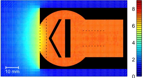
Fig. 4. Simulated density field inside the CONE ionization gauge. Densities are given in units relative to the undisturbed density of the background flowfield.

the wind tunnel to atmospheric flight conditions. However, what we can study in the wind tunnel is the variation of the ram-factor with the angle of attack,α, i.e. the angle between the rocket axis and the velocity vector.

The ram-factors for CONE and TOTAL were measured by exposing them directly to the supersonic jet of the wind tun-nel. The free flow density was directly measured by means of an electronbeam fluorescence technique (Gumbel, 2001b). In Figs. 2 and 3 we present the results of the measured ram-factors for both CONE and TOTAL, respectively, as a func-tion ofα. We only present results from wind tunnel condi-tions 4–7, since the corresponding Mach numbers are clos-est to those during rocket flights (see Table 2). For CONE andα=0, the ram-factor increases with increasing free stream density between 1.6 at the lowest, and 2.4 at the highest den-sity. Since CONE is an open ionization gauge, the ram-factor shows little variation withα. Forα≤60◦, there is hardly any variation detectable. This is a very convenient result because the correction of the atmospheric data due to different an-gles of attack can be neglected (during a typical rocket flight, the angle of attack normally does not exceed 60◦). The TO-TAL measurements show a different behaviour. First of all the ram-factors show more than double the values than the CONE-data, a behaviour which is caused by the closed de-sign of this gauge. Second, the ram-factors show a distinct variation withα. For comparison, we have also plotted solid lines showing a cos(α)-dependence normalized to the mea-sured ram-factor for 0◦. We see that the measurements can be described by such a simple law to a very good

approxima-10 mm

0 2 4 6 8

Fig. 5. Same as for Fig. 4 but for the TOTAL ionization gauge.

tion.

In summary, we conclude that the CONE measurements are independent of the angle of attack, provided thatα ≤ 60◦_{, while the dependence of the ram-factors for TOTAL is} well described by a cosine law.

4.2 Direct Simulation Monte Carlo calculations

As has been explained above, the experimental results for the ram-factors cannot directly be applied to atmospheric flight conditions because of different temperatures in the wind tun-nel flowfield and the atmosphere. Therefore, we have simu-lated the density fields inside the CONE and TOTAL gauge appropriate for atmospheric flight conditions with the Direct Simulation Monte Carlo (DSMC) method (Bird, 1988) in the version of the Stockholm DSMC model (Gumbel, 1997, 2001b). For this model approach, the flow in the vicinity of the two gauges was simulated using two-dimensional ax-ially symmetric grids. While the TOTAL gauge is basically a bucket, the CONE sensor consists of 4 concentrical spheri-cal meshes forming the electrodes of the gauge. In a com-panion paper, Gumbel (2001a) has presented an approach to model the flow through meshes of a given transparency in the framework of the DSMC method. Gumbel has mea-sured the density fields of the flow through meshes of differ-ent transparencies in a wind tunnel experimdiffer-ent under meso-spheric flow conditions and also simulated these flow fields with the DSMC technique. The agreement between measure-ments and simulations was satisfying and we have, therefore, decided to utilize this model approach to simulate the density fields inside the CONE instrument. The basic assumption to model the transmission of the electrodes is to assume that the spherical shells are infinitely thin. Molecules passing through the location of the spheres penetrate the electrodes if a random number between 0 and 1 is less than the given transmission of the electrode (e.g. 0.884 for the outermost grid) and if not, are reflected.

enhanced densities (mean density ratio is of the order of 2) compared to TOTAL (density ratio∼8). On the other hand, the density distribution inside the TOTAL instrument is quite homogenous, whereas inside CONE, there are sharp gradi-ents and inhomogeneities due to the different meshes. Based on flowfield calculations for the whole altitude range of inter-est, i.e. from 70 to 110 km altitude, we have now determined altitude profiles of the ram-factors for both CONE and TO-TAL. While for TOTAL this is an easy exercise due to the homogeneity of the density distribution, more care needs to be taken in the case of the CONE sensor. With the additional knowledge of the spatial distribution of the ionization events in the gauge which we have calculated with the aid of the ion-trace-model SIMION (Dahl, 1995), the ram-factor has been determined by a weighted mean over the ionization volume.

Before we turn to the presentation and discussion of the ram-factor profiles appropriate for atmospheric applications, we state that we have also calculated ram-factors for wind-tunnel conditions. For both CONE and TOTAL, we have determined ram-factors for experiment Nr. 7 (see Table 3 for more details), i.e. for laboratory conditions which are close to flight conditions in the vicinity of the mesopause at alti-tudes of∼90 km (see Table 2). For CONE, we obtain a DSMC result of 1.6±0.1 compared to a measured value of 1.6±0.25. For TOTAL, the Monte Carlo simulations give 4.6±0.1 compared to a measured value of 4.1±0.7. Thus, both for CONE and TOTAL, the simulated and measured ram-factor values agree within the uncertainty of their error bars.

4.3 Validation of DSMC results with falling sphere densi-ties

An independent check of the altitude profiles of calculated ram-factors can be achieved by comparing the uncorrected densities of the ionization gauges with the density measure-ments by falling spheres. All TOTAL/CONE sounding rocket flights were accompanied by at least one falling sphere flight in order to determine meteorological conditions in the mid-dle atmosphere. The falling sphere technique has been de-scribed intensively in the literature (e.g. Schmidlin, 1991). The prime quantity measured is atmospheric density which is deduced from the measured deceleration of the sphere due to the friction with the atmospheric air. Density profiles are achieved from∼95 km down to 30 km, with an altitude res-olution of some kilometers in the upper part of the trajectory (e.g. Schmidlin, 1991; L¨ubken, 1999). The falling sphere profiles used in this paper have been published by L¨ubken and von Zahn (1991) and L¨ubken (1999).

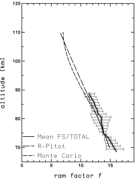
In Fig. 6 we show a height profile of the mean density ratio determined from the comparison of a total of 5 density profiles measured with the CONE instrument, with 7 falling sphere density profiles (in two cases there was one falling sphere shortly before and after the ionization gauge). The error bars indicate the rms variation of the data. In this plot we have also indicated the results of the DSMC simulations. In the altitude range of overlap, the profiles reveal a rather

Fig. 6. Altitude profiles of ram-factors for the CONE instrument once determined numerically with DSMC calculations (dashed line) and once determined from the comparison of CONE and falling sphere measurements (thick solid line). Error bars of the DSMC data represent the statistical uncertainty of the simulations; those of the CONE/falling sphere data represent the rms variation of the seven individual profiles.

good agreement. Note that the apparent small deviation at ∼82 km is not significant, i.e. the profiles still agree within their error bars. This apparent deviation is probably due to the rather crude statistics of only seven simultaneous data sets of CONE and falling sphere measurements. The devia-tion vanishes, for example, in case of TOTAL, where 17 pro-files are available (see below). This demonstrates that indeed the DSMC method is useful in quantitatively determining the ram-factor for the CONE instrument.

Fig. 7. Mean altitude profile of density ratios between TOTAL and falling sphere measurements (thick solid line). Error bars indicate the rms variation of the data. In addition, the results from the DSMC calculations (short dashed line) and a ram-factor calculated with the Rayleigh-Pitot formula (long dashed line) (Shapiro, 1954) are shown.

90 km is expected, as the Rayleigh-Pitot formula is based on continuum mechanics. Therefore, it is approximatly at alti-tudes where the Knudsen number becomes larger than∼0.1 where the Monte Carlo results depart from the Rayleigh-Pitot values.

In summary, we conclude that the excellent agreement of the calculated ram-factors and empirically determined den-sity ratios from falling spheres and ionization gauges sug-gests that we can indeed apply the results of the Monte Carlo simulations to correct the ionization gauge density measure-ments. If we take these correction factors to be exact, then the remaining uncertainty of our density measurements is de-termined by the uncertainty of the laboratory calibration with an upper limit of 2%.

5 Results

We have corrected all the density profiles measured during the rocket flights, listed in Table 1, with the ram-factor files introduced in the last section. The resulting density pro-files have been grouped according to season. Thus, we ob-tain the four sets of density measurements listed in Table 4.

Table 4. Rocket flights used to derive mean seasonal density pro-files.

Time of Year Flights

July/August TURBO-A,TURBO-B,SCT03 SCT06,ECT02,ECT07,ECT12

September/October LT01,LT06,LT13,LT17,LT21 January/March DAT13,DAT50,DAT62,DAT73

DAT76,DAT84,NLTE1

May MSMI03

All the sounding rockets have been launched from the North-Norwegian launch site Andøya (69◦N, 16◦E), except for the flights TURBO-A and TURBO-B, which have been launched from ESRANGE in Northern-Sweden (68◦ N, 22◦ E) and flights DBN01 - DBN03 which have been launched from Biscarrosse in southern France (e.g. Lehmacher and L¨ubken, 1995). Andøya and ESRANGE have nearly the same lat-itude, such that the data can be merged together to derive mean profiles. Our guideline to group the measured profiles was the seasonal variation of densities and temperatures, ear-lier deduced from falling sphere measurements (L¨ubken and von Zahn, 1991; L¨ubken, 1999). While the July/August data and the January/March data fall into the core summer and winter season, respectively, the September/October and the May data have been measured in the transition times from one state to the other (L¨ubken, 1999). Note that we have only used data from rocket flights listed in Table 1 during which the angle of attack did not exceed a limit of∼60◦. For angles of attack larger than this limit, we cannot easily cor-rect for the angular dependence of the ram-factor (see Sect. 4.1 for more details). A listing of mean densities, except for the month May, where only one successful measurement has been performed up until now, is presented in Table 5.

We start with the presentation of the results for the summer flights in July and August. In Fig. 8 we present a summary plot of all seven density profiles. In order to make small scale features on top of the exponential trend of the profiles more easily visible, we have divided all profiles by a reference pro-file from CIRA86 (Fleming et al., 1990). Furthermore, we have calculated the mean of the profiles and indicated the deviation every five kilometer of our data from CIRA86. It turns out that the CIRA86 densities are too low below 80 km altitude, by about 20%. However, above 80 km, we find that CIRA86 densities are too large by about 40%, consistent with the results of L¨ubken (1999).

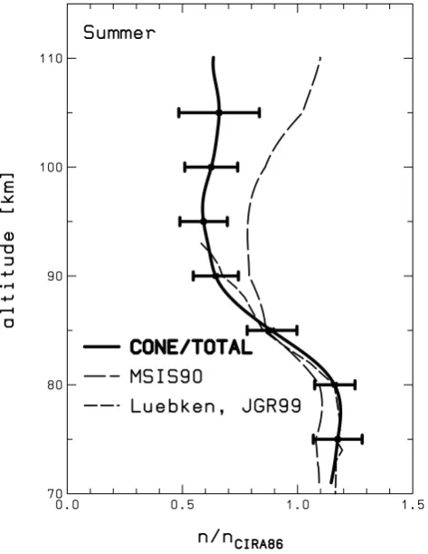
How do our mean summer densities compare to other mea-surements or reference atmospheres? In Fig. 9 we present a comparison of our mean profile with a mean falling sphere profile from L¨ubken (1999) and the reference atmosphere MSIS901(Hedin, 1991). We first note that the agreement of the CONE/TOTAL densities and the falling sphere densities is perfect. Below 85 km, both profiles are merely

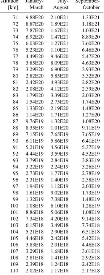
Table 5. Seasonal variation of ionization gauge neutral number den-sities. All densities are given in m−3. Read yEx as y·10x.

Altitude January- July- September-[km] March August October

71 9.88E20 2.10E21 1.33E21 72 8.87E20 1.89E21 1.18E21 73 7.87E20 1.67E21 1.03E21 74 6.92E20 1.47E21 8.89E20 75 6.03E20 1.27E21 7.60E20 76 5.23E20 1.10E21 6.46E20 77 4.49E20 9.46E20 5.47E20 78 3.85E20 8.09E20 4.63E20 79 3.29E20 6.90E20 3.93E20 80 2.82E20 5.85E20 3.32E20 81 2.42E20 4.93E20 2.82E20 82 2.08E20 4.12E20 2.39E20 83 1.79E20 3.39E20 2.03E20 84 1.54E20 2.75E20 1.74E20 85 1.33E20 2.19E20 1.48E20 86 1.14E20 1.71E20 1.27E20 87 9.76E19 1.32E20 1.08E20 88 8.35E19 1.01E20 9.11E19 89 7.15E19 7.65E19 7.65E19 90 6.11E19 5.86E19 6.41E19 91 5.21E19 4.56E19 5.37E19 92 4.44E19 3.59E19 4.52E19 93 3.79E19 2.84E19 3.83E19 94 3.22E19 2.24E19 3.26E19 95 2.73E19 1.77E19 2.78E19 96 2.31E19 1.40E19 2.38E19 97 1.94E19 1.12E19 2.03E19 98 1.61E19 9.02E18 1.73E19 99 1.32E19 7.38E18 1.48E19 100 1.08E19 6.10E18 1.26E19 101 8.86E18 5.06E18 1.08E19 102 7.34E18 4.20E18 9.14E18 103 6.15E18 3.49E18 7.74E18 104 5.21E18 2.90E18 6.51E18 105 4.46E18 2.42E18 5.42E18 106 3.83E18 2.01E18 4.46E18 107 3.29E18 1.68E18 3.61E18 108 2.81E18 1.41E18 2.92E18 109 2.39E18 1.24E18 2.42E18 110 2.02E18 1.17E18 2.17E18

able, and above that the deviation is well within the rms-variability of the CONE/TOTAL measurements, as indicated by the error bars. We further note that below 85 km, MSIS90 represents the correct situation closer than CIRA86. Here, the deviation between the CONE/TOTAL and the MSIS90 data is also within the CONE/TOTAL rms-variation. How-ever, above 85 km, MSIS90 also has densities which are too large, i.e. 20% at 90 km and 40% at 110 km.

The situation changes for the data sets during the transition months of September/October presented in Fig. 10. In this case, the comparison of the CONE/TOTAL data, the MSIS90 data, as well as the falling sphere data shows a close

agree-Fig. 8. All summer density profiles measured with the TOTAL or CONE ionization gauges divided by the appropriate CIRA86 ref-erence profile. The thick line indicates the mean profile of all ion-ization gauge measurements. Furthermore, the deviation between the mean ionization gauge densities and CIRA86 is indicated every 5 km.

ment at least when the rms-variation of the ionization gauge densities is included. We conclude that during this period all of the discussed data sets describe the real mean state of the atmosphere sufficiently well. Only CIRA86 shows sig-nificant deviations of the order of 25% at 85 km and 105 km altitude, respectively.

In the period from January to March (see Fig. 11), all den-sities agree well, except (this time) for the MSIS90 data set, which shows a maximum deviation of nearly 40% at 100 km altitude from the ionization gauge measurements. On the other hand, the natural variability of atmospheric densities at this altitude is also rather large, i.e. on the order of 20%. Yet, the difference between the CONE/TOTAL data and the MSIS90 data is significant.

qual-Fig. 9. Comparison of ionization gauge densities to density pro-files from MSIS90 (Hedin, 1991) and mean falling sphere densities (L¨ubken, 1999) for the core summer months July and August.

ity of our algorithm to correct for the aerodynamical effects described above. While all previously discussed sounding rocket flights had an apogee of approximately 130 km, flight MSMI03 only reached an apogee of 106 km. Hence, the aerodynamical parameters for this flight are different such that the Monte Carlo calculations had to be repeated for this particular rocket flight. The good agreement between the falling sphere and the CONE data emphasizes impressively the quality of the Monte Carlo method.

Apart from this more technical point of view, we would also like to emphasize the discrepancy between the actual CONE measurements and the mean falling sphere profile from L¨ubken (1999). While for all other periods of the year there was a near perfect agreement between the ionization gauge and the mean falling sphere densities, here we find a discrepancy of the order of 15%. This is due to the large natural variability which characterizes the transition period during which the data were taken. It is just at the beginning of May when the atmosphere departs from its stable ‘win-ter state’ and passes over to its ‘summer state’ with steep temporal gradients of atmospheric temperatures in between (L¨ubken, 1999).

Fig. 10. As for Fig. 9 but for the months September and October.

6 Summary

Fig. 11. As for Fig. 9 but for the months January through March. The falling sphere densities have been adopted from L¨ubken and von Zahn (1991).

it turns out that particularly during the summer, the use of CIRA86 or MSIS90 densities to derive, for example, mixing ratios of trace constituents can be wrong by as much as 40%. Finally, it should be emphasized that our results establish the method of measuring absolute neutral air densities with rocket-borne ionization gauges provided that aerodynamic effects are corrected, as described in this paper. Compared to measurements with falling spheres this has the great advan-tage of a real simultaneous common volume measurement with different instruments, as well as a measurement with a higher altitude resolution in the mesopause region (200 m compared to several km), and finally a larger upper altitude limit (i.e. 110 km compared to∼90 km). The last point is especially important during winter when the mesopause has an average altitude of∼100 km and cannot be determined in situ from the falling sphere technique.

Acknowledgements. The authors thank J. All`egre for his excellent support during the wind tunnel experiments and J.C. Lengrand for supporting us to get funded under the Access to Large Scale Fa-cilities activity of the Training and Mobility of Researcher’s pro-gramme of the European commission. We further greatly appreciate C. Unckell’s contribution to this work by developing the ion-trace model for the determination of the actual ionization volume inside the CONE sensor. The rocket flights were supported by the Bun-desministerium f¨ur Bildung, Wissenschaft, Forschung und Tech-nologie under DARA grants 01OE88027 and 50OE9802.

Fig. 12. As for Fig. 9 but for May. The ionization gauge data set comprises only of a single rocket flight in this case. For compar-ison we also show the data of a falling sphere, labeled MSFS02, measured only a few minutes before the sounding rocket flight.

The Editor in Chief thanks R. Goldberg and M. Horanyi for their help in evaluating this paper.

References

Bird, G. A., Aerodynamic effects on atmospheric composition mea-surements from rocket vehicles in the thermosphere, Planet. Space Sci., 36, 921–926, 1988.

Dahl, D. A., SIMION 3D: version 6.0, Ion Source Software, KLACK Inc., Idaho Falls, 1995.

Fleming, E. L., Chandra, S., Barnett, J. J., and Corney, M., Zonal mean temperature, pressure, zonal wind, and geopotential height as functions of latitude, Adv. Space Res., 10(12), 11–59, 1990. Giebeler, J., L¨ubken, F.-J., and N¨agele, M., CONE – a new

sen-sor for in-situ observations of neutral and plasma density fluc-tuations, Proceedings of the 11th ESA Symposium on European Rocket and Balloon Programmes and Related Research, Mon-treux, Switzerland, ESA-SP-355, 311–318, 1993.

Gumbel, J., Rocket-borne optical measurements of minor con-stituents in the middle atmsophere, Ph.D. thesis, Stockholm Uni-versity, 1997.

Gumbel, J., Rarefied gas flows through meshes and implications for atmospheric instruments, Ann. Geophysicae, this issue, 2001a. Gumbel, J., Aerodynamic influences on atmospheric in situ

middle and lower atmosphere, J. Geophys. Res., 96, 1159–1172, 1991.

Hillert, W., L¨ubken, F.-J., and Lehmacher, G., TOTAL: A rocket-borne instrument for high resolution measurements of neutral air turbulence during DYANA, J. Atmos. Terr. Phys., 56, 1835– 1852, 1994.

Lehmacher, G. and L¨ubken, F.-J., Simultaneous observation of con-vective adjustment and turbulence generation in the mesosphere, Geophys. Res. Lett, 22, 2477–2480, 1995.

L¨ubken, F.-J., On the extraction of turbulent parameters from atmo-spheric density fluctuations, J. Geophys. Res., 97, 20385–20395, 1992.

L¨ubken, F.-J., Seasonal variation of turbulent energy dissipation rates at high latitudes as determined by insitu measurements of neutral density fluctuations, J. Geophys. Res., 102, 13441–

13456, 1997.

L¨ubken, F.-J., The thermal structure of the arctic summer meso-sphere, J. Geophys. Res., 104, 9135–9149, 1999.

L¨ubken, F.-J. and von Zahn, U., Thermal structure of the mesopause region at polar latitudes, J. Geophys. Res., 96, 20841–20857, 1991.

Patterson, G. N., Molecular flow of gases, John Wiley & Sons, New York, 1956.

Schmidlin, F. J., The inflatable sphere: A technique for the accurate measurement of middle atmosphere temperatures, J. Geophys. Res., 96, 22673–22682, 1991.

Shapiro, A., The Dynamics and Thermodynamics of Compressible Fluid Flow, vol. I, The Ronald Press Company, New York, 1954. Witt, G., Height, structure and displacements of noctilucent clouds,