POM - QM
FOR WINDOWS
Version 3
Software for Decision Sciences:
Quantitative Methods,
Production and Operations Management
Howard J. Weiss
www.prenhall.com/weiss [email protected]
Table of Contents
Chapter 1: Introduction
Overview...1
Hardware and Software Requirements ...3
Installing the Software ...4
The Program Group ...5
Starting the Program ...6
The Main Screen ...7
Chapter 2: A Sample Problem
Introduction...12Creating a New Problem ...13
The Data Screen ...15
Entering and Editing Data...15
The Solution Screen ...17
Chapter 3: The Main Menu
File ...19 Edit ...25 View ...26 Module ...27 Format ...28 Tools...30 Window...31 Help...32Chapter 4: Printing
The Print Setup Screen...37Information to Print...38
Page Header Information ...39
Page Layout...40
POM-QM for Windows
Chapter 5: Graphs
Introduction...43
File Saving ...44
Print...44
Colors and Fonts ...45
Chapter 6: Modules
Overview...45Aggregate (Production) Planning...46
Assembly Line Balancing/Line Balancing ...57
The Assignment Model ...65
Breakeven/Cost-Volume Analysis ...67
Capital Investment/Financial Analysis ...71
Decision Analysis ...73
Forecasting ...84
Game Theory...99
Goal Programming ...102
Integer and Mixed Integer Programming...106
Inventory ...109
Job Shop Scheduling (Sequencing)/Scheduling ...117
Layout/Process Layout...127
Learning (Experience) Curves ...131
Linear Programming ...134
Location ...140
Lot Sizing...146
Markov Analysis ...151
Material Requirements Planning/Resource Planning ....155
Networks ...162
Productivity...166
Project Management ...167
Quality Control/Process Performance and Quality ...176
Reliability...183
Simulation ...186
Statistics ...189
The Transportation Model ...194
Waiting Lines...198
Work Measurement/Measuring Output Rates...207
Preface
It is hard to believe that POM-QM for Windows (formerly DS for Windows) has been in existence, first as a DOS program and then as a Windows program, for more than 15 years. It seems as if people have been using both minicomputers and Windows forever but, in fact, large-scale Windows usage has occurred for less than a decade. At the time that I finished the original DOS version, few students had personal computers or knew what an Internet service provider (ISP) was. Today, the large majority of students have their own computers, which makes this software even more valuable than it has ever been.
The original goal in developing this software was to provide students with the most user-friendly package available for production/operations management, quantitative methods, management science, and operations research. We are gratified by the response to the four previous DOS versions and two previous Windows versions of POM-QM for Windows,
indicating that we have clearly met our goal.
The first version of this software was a DOS version published in 1989 as PC-POM. Subsequent DOS versions were titled AB:POM. The first Windows version, QM for Windows
(Version 1.0), was distributed in the summer of 1996 whereas a separate but similar program,
POM for Windows (Version 1.1), was first distributed in the fall of 1996. DS for Windows, which contained all of the modules in both POM and QM and also came with a printed manual, was first distributed in 1997. Version 2 of all three programs was created for Windows 95 and distributed in the fall of 1999.
POM-QM for Windows
This is a package that can be used to supplement any textbook in the broad area known as Decision Sciences. This includes Production and Operations Management, Quantitative Methods, Management Science, or Operations Research.
Following is a summary of the major changes included in Version 3. These changes fall into three categories: module enhancements, functionality, and user friendliness.
Module Enhancements
In the aggregate planning module, we have added a model to create and solve a transportation model of aggregate planning. For assembly-line balancing, we have added a display that summarizes the minimum number of stations necessary when using each of the available methods. For decision tables, we have added an output display for various values of alpha when computing the Hurwicz value. Our most exciting new addition is that in decision analysis we now have an easy-to-use graphical user interface to create the decision tree. In addition, we have added a new model for creating decision tables for one-period inventory (supply/demand) problems. In forecasting, we have added a model that allows the user to enter the forecasts in order to run an error analysis. In addition, we have added the MAPE as standard output for all models and added forecast control with computation of the tracking signal. In inventory, we have added the reorder point models for both normal and discrete demand distributions. In job shop scheduling, for one-machine sequencing we have allowed for inclusion of the dates that jobs are received and we have added a display that summarizes the results when using all of the methods. In location, we have added a location cost-volume (breakeven) analysis model. In linear programming we display the input in equation form on the right side of the table and have added an output that has the dual model of the original problem. It is also now possible to print the corner points of a graph. In project management, we display the critical path in red. In quality control, it is now possible to set the center line in the control charts rather than using the mean of the data. We have extended our statistics model to include computations for a list of data, a frequency table, or a probability distribution as well as adding a normal distribution model.
Functionality
expanded to include nearly all of the models. The Windows calculator will be used when found rather than the more primitive calculator that is included with the software. Scroll bars have been added to the forecasting, learning curve and operating characteristic graphs in order to easily display the changes in the graphs as a function of the model parameters.
User Friendliness
As mentioned previously, we have combined all three packages into one package in order that all models will be available to the students – especially students who take both an Operations Management course and a Quantitative Methods course. We still allow for student choice of the menu (POM, QM, or both) to minimize confusion. In addition, in order to improve the understanding of the models we have added separators between models in the model submenu selection menu. We have combined integer and mixed integer programming into one module. We have added an overview tab to the problem creation screen to help describe the options that are available. Manuals (this document) in PDF and Word format have been added so that users may easily access the manual while running the program or print selected pages from the manual. Tutorials that walk you through certain operations step-by-step are included in the Help menu. The examples used in this manual are included in the installation. More user customization options are available in the User Preferences section under the Help menu.
POM-QM for Windows
Acknowledgments
The development of any large scale project such as POM-QM for Windows requires the assistance of many people. I have been very fortunate in gaining the support and advice of students and colleagues from around the globe. Without their help, POM-QM for Windows would not have been as successful as it has been.
In particular, though I would like to thank the students in Barry Render’s classes at Rollins College and the students in my classes at Temple University. These students have always been the first to see the new versions, and over the years several students have offered design features that were incorporated into the software. Other design features were developed in response to comments sent to me from users of the DOS versions and Windows versions 1 and 2. I am extremely grateful for these comments; they have immensely helped the evolution and continuous improvement of POM-QM for Windows.
Several changes in the software were put into place in version 3 as a result of the comments of Philip Entwistle, Northampton Business School. The original version of the POM for Windows and QM for Windows software was reviewed by Dave Pentico of Duquesne University, Laurence J. Moore of Virginia Polytechnic Institute and State University, Raesh G. Soni of Indiana University of Pennsylvania, Donald G. Sluti of the University of Nebraska at Kearney, Nagraj Balachandran of Clemson University, Jack Powell of the University of South Dakota, Sam Roy of Morehead State University, and Lee Volet of Troy State University. Their comments were very influential in the design of the software that has been carried over to the new version.
Discussions with Fred Murphy and the late Carl Harris have been very useful to me, especially in the mathematical programming and queueing modules.
There are several individuals at Prentice Hall to whom I must give special thanks. Rich Wohl and Tom Tucker are the editors with whom I had worked on this project for the first six versions. Not all editors have their keen understanding of computers, software, texts, students, and professors. Without this understanding and vision,
POM-QM for Windows would still be a vision rather than a reality. My current editors, Alana Bradley and Mark Pfaltzgraf, have been instrumental in getting this version to market. Fellow Prentice Hall authors, including Jay Heizer, Barry Render, Ralph Stair, and Chuck Taylor have helped me to develop the DOS versions and to make the transition from the DOS product to the current Windows products and to improve the Windows product. I am grateful for their many suggestions and the fact that they chose my software as the software to accompany their texts. The support, encouragement, and help from all of these people are very much appreciated. Nancy Welcher provides the support of the Prentice Hall Web pages that are maintained for my products. Finally, I would like to express my appreciation to Debbie Clare who has been the marketing manager for my software.
Chapter 1
Introduction
Overview
Welcome to Prentice Hall’s Decision Science software package: POM-QM for Windows (also known as POM for Windows and QM for Windows). This package is the most user-friendly software package available in the fields of production and operations management, quantitative methods, management science, or operations research. POM-QM for Windows has been designed to help you to better learn and understand these fields. The software can be used either to solve problems or to check answers that have been derived by hand. POM-QM for Windows contains a large number of models, and most of the homework problems in POM textbooks or QM textbooks can be solved or approached using POM-QM for Windows.
In this introduction and the next four chapters, the general features of the software are described. You are encouraged to read them while running the software on your computer. Chapter 6 contains the description of the specific models and applications available in POM-QM for Windows.
You will find that the software is very user friendly as a result of the following features.
Standardization
The graphical user interface for the software is a standard Windows interface. Anyone familiar with any standard spreadsheet, word processor, or presentation package in Windows easily will be able to use the software. This standard interface includes the customary menu, toolbar, status bar, and help files of Windows programs.
POM-QM for Windows
File storage and retrieval is simple. Files are opened and saved in the usual Windows fashion and, in addition, files are named by module, which makes it easy to find previously saved files.
Data and results, including graphs, can be easily copied and pasted between this application and other Windows applications.
Flexibility
There are several preferences that the user can select from the Help, User Information menu. For example, the software can be set to automatically save a file after data has been entered or to automatically solve a problem after data has been entered
The menu of modules can be either a menu that lists only POM model, a menu that list only QM models, or a menu that lists all available models.
The user can select the desired output to print rather than having to print everything. In addition, several print formatting options are available.
The screen components and the colors can be customized by the user. This can be particularly effective for overhead data shows.
User-oriented design
The spreadsheet-type data editor makes data entry and editing extremely easy. In addition, whenever data is to be entered, there is a clear instruction given on the screen describing what is to be entered. Also, when data is entered incorrectly, a clear error message is displayed.
It is easy to change from one solution method to another in order to compare methods and answers. In several cases, this is simply a one-click operation. In addition, intermediate steps are generally available for display.
The display has been color coded so that answers appear in a different color from data.
Textbook customization
Chapter 1: Introduction
User support
Updates are available on the Internet through the Prentice Hall Web site for this book, www.prenhall.com/weiss, and help is available by contacting [email protected].
What all of this means to you is that, with a minimal investment of time in learning the basics of POM-QM for Windows, you will have an easy-to-use means of solving problems or checking your homework. Rather than being limited to looking at the answers in the back of your textbook, you will be able to see the solutions for most problems. In many cases, the intermediate steps are displayed in order to help you check your work. In addition, you will have the capability to perform sensitivity analysis on these problems or to solve bigger, more interesting problems.
Hardware and Software Requirements
Computer
The software has minimal system requirements. It will run on any IBM PC compatible Pentium machine with at least 8 MB RAM and operating Windows 2000, Windows NT, Windows ME, or Windows XP.
Disk Drives/CD-ROM
The software is provided on a CD. This requires a CD-ROM drive.
Monitor
The software has no special monitor requirements. Different colors are used to portray different items, such as data and results. All messages, output, data, and so on will appear on any monitor. Regardless of the type of monitor you use, the software has the capability that allows you to customize colors, fonts and font sizes in the display to your liking. This is extremely useful when using an overhead projection system. These options are explained in Chapter 3 in the section titled Format.
Printer
POM-QM for Windows
Typographic conventions in this manual
1. Boldface indicates something that you type or press.
2. Brackets, [ ], name a key on the keyboard or a command button on the screen. For example [F1] means Function key F1, whereas [OK] means the “Okay” button on the screen.
3. [Return], [Enter], or [Return/Enter] indicate the key on your keyboard that has one of those names. The name of the key varies on different keyboards and some even have both keys.
4. Boldface and the capitalized first letter of a term refer to a Windows menu command. For example, File refers to the menu command.
5. All capitals refers to a toolbar command such as SOLVE.
Installing the Software
In the directions that follow, the hard drive is named C: and the CD-ROM is drive D:. The software is installed in the manner that most programs designed for Windows are installed. For all Windows installations, including this one, it is best to be certain that no programs are running while you are installing a new one.
Insert the CD with POM-QM for Windows in drive D:. After a little while, the installation program should begin automatically. If it does not, then
a. From the Windows Start Button select, Run.
b. Browse the CD for D:setup.pomqmv3.exe (case does not matter). c. Press [Enter] or click on [OK].
Follow the setup instructions on the screen. Generally speaking, it is simply necessary to click [NEXT] each time that the installation asks a question.
Default values have been assigned in the setup program, but you may change them if you like. The default folder is C:\Program Files\POMQMV3.
Chapter 1: Introduction
If you have the CD from the Operations Management, 8e textbook by Heizer and Render or the CD from the Operations Management, 8e textbook by Krajewski, Ritzman and Malhotra, the software will automatically be installed as POM for Windows and customized to the textbook. If you have the CD from Quantitative Analysis by Render, Stair and Hanna or the CD from Introduction to Management Science by Taylor, the software will automatically be installed as QM for Windows. If you have the POM-QM for Windows CD rather than a CD from the back of your textbook you can customize the software to the textbooks by using Help, User Information.
One option that the installation will question you about is whether you want to be able to run the program by double clicking on the file name in File Explorer. If you say “yes”, then the program will associate the proper extensions with the program name. This is generally very useful.
Please note that the software installs some files to the Windows system directory. The installation will back up any files that are replaced if you select this option.
If you see a message saying that something is wrong during installation and you have the option of ignoring it, choose this option. The program will likely install properly anyway. The message usually indicates that you are running a program or have run a program that shares a file with this software package. If you have any installation or operation problems, the first place to check is the download page at www.prenhall.com/weiss.
Installing and Running on a Network
With the written permission of Prentice Hall, it is permissible to install the software to a network only if each student has purchased an individual copy of the software. That is, each student must possess his or her own licensed copy of the CD in order to install the software on a network.
The Program Group
POM-QM for Windows
Help is available from within the program, but if you want to read some information about the program without starting it first, use the POM-QM for Windows 3 Help
icon.
The program group contains one icon named Prentice Hall Web Site Gateway. If you have an association for HTML files with a Web browser (e.g., Netscape or Internet Explorer), this document will point you to program updates.
Finally, the software comes with a Normal Distribution Calculator. The calculator is on the Tools menu of the program but also can be used as a stand-alone program without having to open POM-QM for Windows.
To uninstall the program use the usual Windows uninstall procedure (Start, Settings, Control Panel, Add/Remove Programs). The programs will be removed but the data files will not; they will have to be deleted using My Computer or File Explorer if you wish to do so.
In addition to the Start menu, the installation will place a shortcut to the program on the desktop. The icon appears as one of the three icons displayed below depending on the exact CD being used. Whichever desktop icon has been installed is the icon that can be used to easily begin the program.
Starting the Program
Chapter 1: Introduction
Name
The name of the licensee will appear in the display. This should be your name if you are running on a stand-alone computer or the network name if you are running on a network.
Version Number
One important piece of information is the version number of the software. In the example, the version is 3.0 and this manual has been designed around that number. Although this is version 3.0 there is also detailed information about the program version that can be found using Help, About (displayed at the end of Chapter 3). In particular, there is a build number. If you send e-mail asking for technical support, you should include the build number with the e-mail.
Note: If the program has been registered as being in a public lab or on a network then at this point the opening screen will change and give you the opportunity to enter your name. This is useful when you print your results.
The program will start in a couple of seconds after the opening display appears.
The Main Screen
The second screen that appears is an empty main menu screen. The first time that this screen appears, a Tip of the Day form will appear as displayed below. If you don’t want the Tip of the Day to appear each time, uncheck the box at the lower left of the form. If you change your mind later and want to see the Tip of the Day, go to the
POM-QM for Windows
Please notice the background in the middle of the screen. This is referred to as a gradient. This gradient appears whenever the main screen is empty and it appears on other screens in the software. You may customize the display of the gradient by using
Format, Colors as explained in Chapter 3.
Chapter 1: Introduction
The top of the screen shows the standard Windows title bar for the window. At the beginning the title is POM-QM for Windows (or POM for Windows or QM for Windows). If you are using a Prentice Hall text the names of the authors of the texts should appear in this title bar at the beginning of the program as shown in the figure on the previous page. (If not, go to Help, User Information.) The title bar will change to include the name of the file when a file is loaded or saved as shown above. On the left of the title bar is the standard Windows control box and on the right are the standard minimize, maximize, and close buttons for the window-sizing options.
Below the title bar is a bar that contains the main menu. The menu bar is very conventional and should be easy to use. The details of the menu options of File, Edit, View, Module, Format, Tools, Window, and Help are explained in Chapter 3. At the beginning of the program, the Edit option is not enabled, because there is no data to edit. The Window option is also disabled, because this refers to results windows and there are as yet no results. Although the menu appears in the standard Windows position at the top of the screen, it can be moved if you like by clicking on the handle on the left and dragging the mouse.
POM-QM for Windows
(balloon help or tool tip) appears on the screen. As with most software packages, the toolbar can be hidden if you so choose (right click on any of the toolbars or use View, Toolbars, Customize). Hiding the toolbar allows for more room on the screen for the problems. As is the case with most toolbars, they float. In order to reposition any of the toolbars, simply click on the handle on the left and drag.
One very important tool on the standard toolbar is the SOLVE tool on the far right of the toolbar. This is what you press after you have entered the data and you are ready to solve the problem. Alternatively, you may use File, Solve or press the [F9]
key. Please note that after pressing the SOLVE tool, this tool will change to an EDIT tool. This is how you go back and forth from entering data to viewing the solution. For two modules, linear programming and transportation, there is one more command that will appear on the standard toolbar. This is the STEP tool (not displayed in the figure), and it enables you to step through the iterations, displaying one iteration at a time.
Below the standard toolbar is a format toolbar. This toolbar is very similar to the toolbars found in Excel, Word, and WordPerfect. It too can be customized, moved, hidden, or floated.
There is one more toolbar, and its default location is at the bottom of the screen. This bar is a utility bar and it contains six tools. The tool on the left is named MODULE. A module list can appear in two ways — either by using this tool or the Module option on the main menu. The next tool is named PRINT SCREEN, and it is there to emulate the old print screen function in DOS. The next two tools will load files in alphabetical order either forward or backward. This is very useful when reviewing a number of problems in one chapter, such as the sample files that accompany this manual. The two remaining tools allow files to be saved as Excel or HTML files.
Chapter 1: Introduction
table background. The caption colors, table colors, and background color can be changed by using Format, Colors, as explained in Chapter 3.
Above the data table is an area named the extra data bar for placing extra problem information. Sometimes it is necessary to indicate whether to minimize or maximize, sometimes it is necessary to select a method, and sometimes some value must be given. These generally appear above the data. On the right of the extra data panel is an instruction panel. There is always an instruction here to help you to determine what to do or what to enter. When data is to be entered into the data table, this instruction will explain what type of data (integer, real, positive, etc.) is to be entered. The instruction location can be changed by using the View option.
There also is a form for annotating problems. A comment may be placed here. When the file is saved, the comment will be saved; when the file is loaded, the comment will appear and the comment may be printed if so desired.
POM-QM for Windows
Chapter 2
A Sample Problem
Introduction
In this chapter, a sample problem is examined from beginning to end in order to demonstrate how to use the package. Although not all problems or modules are identical, there is enough similarity among them that seeing one example will make it very easy to use any module in this software. As mentioned in the introduction, the first instruction is to select a module to begin the work.
In the preceding figure, the modules are displayed as they are listed when you use the MODULE tool on the utility bar (as opposed to the Module option in the main menu at the top).1 As you can see, there are 29 modules available. They are divided into three groups. The models in the first group typically are included in all POM and QM books, whereas the models in the second group typically appear only in POM books, and the models in the third group appears only in QM texts. The models are divided in
Chapter 2: A Sample Problem
this fashion so that you will understand it is completely fine to ignore POM-only modules if you have a QM course and vice versa.
If you choose the Module option from the main menu, you get the same modules listed in a single list in alphabetical order. (This is displayed in Chapter 3.) You have the option on this menu to display only the POM modules or only the QM modules.
Creating a New Problem
Generally, the first menu option that will be chosen is File, followed by either New, to create a new data set, or Open, to load a previously saved data set. In the figure that follows, the creation screen that is used when a new problem is started is displayed. Obviously, this is an option that will be chosen very often. The creation screens are similar for all modules, but there are slight differences that you will see from module to module.
POM-QM for Windows
For many modules, it is necessary to enter the number of rows in the problem. Rows will have different names depending on the module. For example, in linear programming, rows are “constraints”, whereas in forecasting, rows are “past periods”. At any rate, the number of rows can be chosen with either the scrollbar or the text box. As is usually the case in Windows, they are connected. As you move the scrollbar, the number in the text box changes; as you change the text, the scrollbar moves. In general, the maximum number of rows in any module is 90. There are three ways to add or delete rows or columns after the problem has been created. You may use the options in the Edit menu; you may right click on the data table, which will bring up both copy and insert/delete options; or, to insert a row or insert a column , you may use the tools on the toolbar.
This program has the capability to allow you different options for the default row names. Select one of the six option buttons in order to indicate which style of default naming should be used. In most modules, the row names are not used for computations, but you should be careful because in some modules (most notably Project Management and Material Requirements Planning) the names might be relevant to the computations. In most modules, the row names can be changed by editing the data table.
Many modules require a number of columns. This is given in the same way as the number of rows. The program gives you a choice of default values for column names in the same fashion as row names but on the tab Column Names.
An overview tab is included on the creation screen in this version of the software. The overview tab gives a brief description of the models that are available and also gives any important information regarding the creation or data entry for that module.
Chapter 2: A Sample Problem
When you are satisfied with your choices, click on the [OK] button. At this point, a blank data screen will appear as in the following figure. Screens will differ module by module but they will all resemble the following screen.
The Data Screen
The data screen was described briefly in Chapter 1. It has a data table and, for many models, there is extra information that appears above the data table follows.
Entering and Editing Data
After a new data set has been created or an existing one has been loaded, the data can be entered or edited. Every entry is in a row and column position. You navigate through the spreadsheet using the cursor movement keys (or the mouse). These keys function in a regular way with one very useful exception — the [Enter] key.
POM-QM for Windows
cursor will move to the cell with a “0" in the next row. It is possible to set the cursor to go to the first cell, the one with the name in it, by using Help, User Information.
In addition, if you use the [Enter] key to enter the data, after you are done with the last cell, the program will automatically solve the problem (saving you the trouble of clicking on the SOLVE tool). This behavior can be adjusted by using Help, User Information and, in addition, if you want the program to automatically prompt you to save the file when you are done entering data, this too can be accomplished through
Help, User Information.
The instruction frame on the screen contains a brief instruction describing what is to be done. There are essentially three types of cells in the data table.
One type is a regular data cell into which you enter either a name or a number. When entering names and numbers, simply type the name or number, then press the [Enter]
key, one of the direction keys, or click on another cell. If you type an illegal character, a message box will be displayed indicating so.
A second type is a cell that cannot be edited. For example, the empty cell in the upper left-hand corner of the table can not be edited. (You actually could paste into the cell.)
A third type is a cell that contains a drop-down box. For example, the signs in a linear programming constraint are chosen from this type of box, as shown in the following illustration. To see all of the options, press the arrow on the drop-down box.
When you are finished entering the data, press the SOLVE tool on the toolbar or use
Chapter 2: A Sample Problem
The Solution Screen
An important thing to notice is that there is more solution information available than the one table displayed. This can be seen by the icons given at the bottom. Click on these to view the information.
Alternatively, when you solve the problem, the form below can be set to appear on top of the solution through Help, User Information.
POM-QM for Windows
If you click on the OPTIONS button you can set up the behavior of the software when a problem is solved. The options are as follows:
The first option simply displays the solution. The next three options remind you that more results may exist than the one window displayed. The second option displays the Solutions Window, which contains a brief description of each solution Window. The third option automatically drops down the Window menu. These options can be reset using Help, User Information.
It is generally at this point that, after reviewing the solution, you would choose to print both the problem and solution.
Chapter 3: The Main Menu
Chapter 3
The Main Menu
File
File contains the usual options that one finds in most Windows programs, as seen in the figure that follows.
These options are now described.
New
POM-QM for Windows
Open
Open is used to open or load a previously saved file. File selection is the standard Windows common dialog type. An example of the screen for opening a file follows. Notice that the extension for files in the software system is given by the first three letters of the module name. For example, all forecasting files have the extension *.for. (The exceptions are assembly-line balancing (*.bal) and layout (*.ope) because of conventions in previous versions, and productivity (*.prd) to avoid a conflict with project management.). When you go to the Open File dialog, the default value is for the program to look for files of the type in this module. This can be changed at the bottom left, where it says “Files of type.” Otherwise, file opening and saving is quite normal. The drive or folder can be changed with the drive/folder drop-down box, a new directory may be created using the new button at the top, and details about the files may be seen by using the details button at the top right.
It is possible to use Help, User Information to set the program to automatically solve any problem when it gets loaded. This way, if you like, you can be looking at the solution screen whenever you load a problem rather than at the data screen.
Save
Chapter 3: The Main Menu
Save as
Save as will prompt you for a file name before saving. This option is very similar to the option to load a data file. When you choose this option, the Windows Common Dialog Box for Files will appear. It is essentially identical to the one previously shown for opening files.
The names that are legal are standard Windows file names. In addition to the file name, you may preface the name with a drive letter (with its colon) or path designation. The software will automatically append an extension to the name that you use. As mentioned previously, the extension is the first three letters of the module name. You may type file names in as uppercase, lowercase, or mixed. Examples of legal file names are
sample, sample.tra, c:myFile, c:\myCourse\test, and myproblem.example.
POM-QM for Windows
Save as Excel File
The software has an option that allows you to save most (but not all) of the problems as Excel files. The data is transported to Excel and the spreadsheet is filled with formulas for the solutions. In some cases, Excel’s Solver may be required in order to get the solution.
For example, following is the output from a waiting line model. The left-hand side has the data, whereas the right-hand side has the solution. Notice the color-coding of answer vis-à-vis data.
Chapter 3: The Main Menu
Save as HTML
Any table, either data or solution, may be saved as an HTML file, as shown in the following figure for the waiting line example.
If more than one table is on the screen when this option is selected, the active table is the one that is saved.
Print will display a Print Setup screen. Printing options are described in Chapter 4. Both Save and Print act slightly differently if a graph is being displayed at the time that you use Print or Save.
Print Screen
Print Screen will print the screen as it appears. Different screen resolutions may affect the printing. Printing the screen is more time consuming than a regular print. Use this option if you need to demonstrate to your instructor exactly what was on the screen at the time.
Solve
POM-QM for Windows
[F9] key. Also, if the data is entered in order (top to bottom, left to right, using
[Enter]), the program will solve the problem automatically after a value is entered into the last cell.
After solving a problem, the Solve option will change to an Edit option on both the menu and the toolbar. This is the way to go back and forth between data and solutions. Note that Help, User Information may be used to set the program to automatically maximize the solution windows if so desired.
Step
For the linear programming and transportation modules, a Step option (not displayed in the preceding figure) will appear in the File menu and on the toolbar.
Exit
The next option on the File menu is Exit. This will exit the program. You will be asked if you want to exit the program. You can eliminate this question by using Help, User Information.
Last Four Files
Chapter 3: The Main Menu
Edit
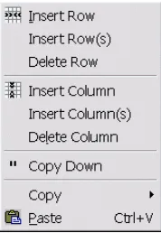
The commands under Edit can be seen in the following illustration. Their purposes are threefold. The first six commands are used to insert or delete rows or columns. The second type of command is useful for repeating entries in a column, and the third type is for cutting and pasting between Windows applications. It is also possible to enable the insert/delete and copy options by right clicking on the data or solution table.
Insert Row inserts a row after the current row, and Insert Column inserts a column after the current column. Insert Rows(s) and Insert Columns(s) ask you how many columns or rows you would like to insert after the current row or column.
Delete Row deletes the current row, and Delete Column deletes the current column.
Copy Entry Down Column
The Copy Down command is used to copy an entry from one cell to all cells below it in the column. This is not often useful, but it can save a great deal of work when it is.
Copy
Copy has five options available. It is possible to copy the entire table, the current row, or the current column to the clipboard. It is possible to copy from the data table or any of the solution tables. Whatever is copied can then be pasted into this program or some other Windows program. (The copy tool in the toolbar copies the entire table.) If you are at the solution stage, the copying will be for the table that is active.
POM-QM for Windows
Paste
Paste is used to paste in the current contents of the clipboard. When pasting into
POM-QM for Windows, the pasting begins at the current cursor position. Thus, it is possible to copy a column to a different column beginning in a different row. This could be done to create a diagonal. It is not possible to paste into a solution table, although, as indicated previously, it is possible to copy from a solution table.
Note: Right clicking on any table will bring up Copy options and if the table is the data table it will also bring up the insert and delete options.
View
View has several options that enable you to customize the appearance of the screen.
The Toolbars menu contains two options. The toolbar can be customized (as can most Windows toolbars) or the toolbar can be reset to its original look.
The Instruction bar can be displayed at its default location in the extra data panel, above the data, below the data, as a floating window, or not at all. The Status Bar
display can be toggled on or off.
Full Screen turns all of the bars (toolbar, command bar, instruction, and status bar) on or off.
Zoom generates a small form allowing you to reduce or increase the size of the columns. It is easier to use the zoom tool on the standard toolbar.
Colors can be set to Monochrome (black and white) or from this state to their
Chapter 3: The Main Menu
Module
A drop-down list with all of the modules in alphabetical order will appear. The MODULE tool on the utility toolbar below the data area is a second way to get a list of modules. At the bottom of the list are options for indicating whether you want to display only the POM modules (as displayed), only the QM modules, or all of the modules as the following display shows.2
POM-QM for Windows
Format
Format has several options for the display of data and solution tables, as can be seen in the following illustration. In addition, there are some additional format options available in the format toolbar.
Colors
Chapter 3: The Main Menu
The first tab is for setting the colors in the data table, and the second tab is for setting the colors in the solution tables. That is, it is possible to have the displays of the data and the display of the results appear differently, which can be helpful. For either the data or the results, you may set the background and foreground colors for rows to alternate by using the odd and even options. This makes reading long tables easier.
In order to set the colors, first select the table property that you want to set, then select foreground or background if applicable, then select rows if applicable, and then click on the color. For example, click on Body, Foreground, Odd, and then click on the red color box and the foreground for every other row will become red. The changes here will be maintained throughout until you return to this screen and reset the colors. If you want to make changes in only one table for one problem, it may be easier to use the toolbar options for foreground and background . Also, the foreground and background color selection tools, as well as the bold, italic, and underline tools, may be used on individual columns if you select these columns before pressing on the tool.
The third tab allows you to customize the colors in the panels (status, instruction). The fourth tab can be used to set the gradient that appears on several of the screens (problem creation, empty data screen), and the fifth tab allows you to reset the colors to their original (factory) settings.
Other Format Options
The font type, style, and size for all tables can be set. Zeros can be set to display as blanks rather than zeros in the data table. The grid line display can be set to horizontal, vertical, both, or none. The problem title that appears in the data table, and which was created at the creation screen, also can be changed .
In order to give some idea of the extensive formatting capabilities available, following is displayed a sample of an overly formatted screen.
POM-QM for Windows
named “Cippy” was selected and the background tool on the toolbar was used to reset the colors for this column only, then “Bruce” and “Lauren” were selected and the Bold and Italic tools on the toolbar were used. Finally, “Brian” was selected and the foreground tool was used.
Returning to the Format menu, observe that the table can be squeezed or expanded . That is, the column widths can be decreased or increased. Each press of the tool changes the column widths by 10 percent. This is very useful if (results) tables are wider than the screen. The toolbar has the zoom option, which also may be used for resizing the column widths.
Note: All tables can have their column widths changed by clicking on the line separating the columns and dragging the column divider left or right. Double clicking on this line will not automatically adjust the column width as it does in Excel.
Number of decimals, Comma and Fixed are used to format the displayed or printed output. The Comma option displays numbers greater than 999 with a comma. The Number of decimals drop-down box controls the maximum number of decimals displayed. If you have it set to “00," then .333 would be displayed as .33 whereas 1.5 would be displayed as 1.5. If you turn on the Fixed (decimal) option, then all numbers would have 2 decimals. Thus 1.5 would be displayed as 1.50 and align with 1.33.
The input can be checked or not. It is a good idea to always check the input, but not checking allows you to put entries into cells that otherwise could not be put there.
The last option of Insert/Delete takes you to the Edit menu.
Tools
The software should find the Windows calculator if you select the Calculator
Chapter 3: The Main Menu
There is an area available to Annotate problems. If you want to write a note to yourself about the problem, select Annotate. The note will be saved with the file if you save the file. An example of annotation appears in Chapter 1. In order to eliminate the annotation completely, the box must be blank (by deleting) and then the file must be resaved. When you print, you have an option to print the note or not.
Window
A sample of the Window options appears in the next illustration. This menu option is enabled only at the solution screen. Notice that in this example there are six different output screens that can be viewed. The number of windows depends on the specific module and problem.
Following is a display of the screen after using the Tile option from the Window
POM-QM for Windows
Help
The Help options are displayed next.
Chapter 3: The Main Menu
anything to be warned about regarding the option, it will appear on the help screen as well as in Chapter 6 of this manual.
Tip of the Day
The Tip of the Day will be displayed. From this option, it is possible to set the tip to display all of the time or not to display at all.
E-mail support
E-mail support uses your e-mail to set up a message to be sent to Prentice Hall. The first step is to click on the main body of the message and then to paste (CTRL-V or SHIFT-INS) the information that the program has created into the body of the e-mail.
Program Update
Program Updates points you to www.prenhall.com/weiss. Updates are on the download page.
Manual
The program comes with this manual in both PDF form and as a Word document. The PDF manual requires Adobe acrobat reader, which is available free through http://www.adobe.com/.
Tutorials
POM-QM for Windows
User Information
Chapter 3: The Main Menu
The second tab is used to set several of the options that have been discussed to this point.
POM-QM for Windows
About POM-QM for Windows
Chapter 4: Printing
Chapter 4
Printing
The Print Setup Screen
After selecting Print from the menu (or toolbar), the Print Setup screen will be displayed as shown in the accompanying figure. There are several options on this screen that are divided over five tabs. The first tab is shown in the figure below.
POM-QM for Windows
Information to Print
The options in the frame depend on whether Print was selected from the data screen or from the solution screen. From the data screen, the only option that will appear is to print the data. However, from the solution screen there will be one option for each screen of solution values.
For example, in the preceding linear programming example, there are six different output displays as well as an available graph and annotation because this file had a note attached. You can select which of these will be printed. In general, the data is printed when printing the output, and, therefore, it is seldom necessary to print the data, meaning that all printing can be performed after the problem is solved.
Tables versus Equations
For mathematical programming types of modules, there is an option available about the style of printing. The problem can be printed in regular tabular form or in equation form. Examples of each follow.
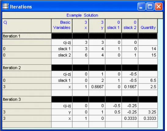
Tabular Form
Results ---
x y RHS Dual Maximize 3 3 labor hours 3 4 <= 14 0.5 material (pounds) 6 4 <= 15 0.25
Equation Form
Results --- OPTIMIZE: 3x + 3y
labor hours:+ 3x + 4y <= 14
material (pounds):+ 6x + 4y <= 15
Printing Graphs
If you select to print the graphs, the software will allow you to select which graphs should be printed. For example, Project Management results include three Gantt charts and a precedence graph. You can select which graphs you would like from the list that is presented in the following figure.
Chapter 4: Printing
If all you want is one of the graphs, it is also possible to do your graph printing from the graph screen (described in the next chapter) rather than from the results screen. Furthermore, if you want to control the size of the printed graph, use the options presented in the next chapter.
Page Header Information
POM-QM for Windows
Page Layout
The tab for page layout displays as follows.
Print As
There are two styles of printing that may be used. The most common and fastest way to print is as ASCII (plain text). In addition, you may also print a grid similar to the one that appears on the screen. Thus, you may format the grid, then go to the print option, and print a highly formatted grid. The formatted grids take longer to print than the plain text.
Paper Orientation
The paper can be printed in upright fashion (portrait) or it can be printed sideways (landscape) if you need more space for columns.
Answers
Answers can be bold, italic, color, or any combination of the three. Do not opt for color if you do not have a color printer. In fact, if you set the printing to use color on a black/white printer, the color answers generally appear lighter! This usually is not the desired characteristic.
Spacing
Chapter 4: Printing
Margins
The left, right, top, and bottom margins can be set from 0 to 1 inch in increments of .1 inches. The margin is above or beyond any natural margin that the printer itself has. Margins of 0 allow for the most printing across the page.
Maximum Column Widths
The maximum widths of the columns (in characters) can be set. The leftmost column which is usually names, can be set separately from the other columns. This is useful if you want to compress tables.
Printer Options
The tab for the printer options is as follows.
Print to and If File Already Exists
It is possible to print to the printer or to print to a file. If you print to a file you will be asked for a file name. Any name can be given. You also have the option of adding the printing to a file that was already there (appending) or erasing a file before printing (replace file).
POM-QM for Windows
Print Timing
Printing can occur each time that you use Print or at the end, when everything will be printed at once. Printing each time is generally preferable, but there are some situations where you want to wait until the end because this may save paper or minimize the number of trips to a network printer.
Change Default Printer
Chapter 5: Graphs
Chapter 5
Graphs
Introduction
POM-QM for Windows
When a graph is opened, two things occur. First the graph will be displayed covering the entire area below the extra data; and second, some of the menu options will change or execute differently.
File Saving
The file save option both under File on the main menu and on the toolbar will save the (active) graph rather than saving the file. The file may still be saved by using File, Save as or by going to a results window other than the graph window.
Print now will print the graph rather than presenting the general print setup screen. The print graph options are shown in the following figure. The graph can be printed in two sizes, and can be printed as either portrait (8.5 by 11) or landscape (11 by 8.5). Small graphs can be printed at the top or bottom of the page. Thus, there is slightly more customization of graph printing available through this method than when printing the graphs as part of the output, as described in the previous chapter.
Colors and Fonts
Chapter 6: Modules
Chapter 6
Modules
Overview
In this chapter, each of the 29 modules is detailed3. The input required for each module, the options available for modeling and solving, and the different output screens and reports that can be seen and printed are explained. Recall that the menu can be set to display only POM modules, only QM modules or all modules. For modules that are in both the POM and QM menus we display the POM-QM for Windows icon:
For all modules that are in the POM-only menu, we display the POM for Windows icon and for all modules that are in the QM-only menu we display the QM for Windows icon:
For example, in the first module, aggregate planning, which begins on the next page, the POM icon is displayed because aggregate planning is typically a topic in Operations Management courses but not in Management Science courses and thus appears in the POM-only menu. Finally, the examples used in this manual have been installed in the Examples folder in the POM-QM for Windows folder (Program Files\POMQMV3).
POM-QM for Windows
Aggregate (Production) Planning
Production planning is the means by which production quantities are prepared for the medium term (generally 1 year). Aggregate planning refers to the fact that the production planning is usually carried out across product lines. The terms aggregate planning and production planning are used interchangeably. The main planning difficulty is that demands vary from month to month. Production should remain as stable as possible, yet it should maintain minimum inventory and experience minimum shortages. The costs of production, overtime, subcontracting, inventory, shortages, and changes in production levels must be balanced.
In some cases, aggregate planning problems might require the use of the transportation or linear programming modules. The second submodel in the aggregate planning module creates and solves a transportation model of aggregate planning for cases where all of the costs are identical. The transportation model is also available as one of the methods for the first submodel.
The Aggregate Planning Model
Production planning problems are characterized by a demand schedule, a set of capacities, various costs, and a method for handling shortages. Consider the following example.
Example 1: Smooth Production
Consider a situation where demands in the next four periods are for 1200, 1500, 1900, and 1400 units. Current inventory is 0 units. Suppose that regular time capacity is 2000 units per month and that overtime and subcontracting are not considerations. The costs are $8 for each unit produced during regular time, $3 for each unit held per period, $4 for each unit short period, $5 for each unit by which production is increased from the previous period, and $6 for each unit by which production is decreased from the previous period. The screen for this example follows.
In addition to the data, there are two considerations — shortage handling and the method to use for performing the planning. These appear in the area above the data.
Chapter 6: Modules
if you cannot satisfy the demand in the period in which it is requested, the demand disappears. This option is above the data table.
Methods. Six methods are available, which will be demonstrated. Please note that smooth production accounts for two methods.
Smooth production will have equal production in every period. This yields two methods because the production can be set according to the gross demand or the net demand (gross demand minus initial inventory).
Produce to demand will create a production schedule that is identical to the demand schedule.
Constant regular time production, followed by overtime and subcontracting if necessary. The lesser cost method will be selected first.
Any production schedule is available in which case the user must enter the amounts to be produced in each period.
The transportation model.
Quantities
Demand. The demands are the driving force of aggregate planning and these are given in the second column.
POM-QM for Windows
quantities. When deciding whether to use overtime or subcontracting, the program will always first select the one that is less expensive.
Costs
The costs for the problem are all placed in the far right column of the data screen.
Production costs — regular time, overtime, and subcontracting. These are the per-unit production costs depending on when and how the unit is made.
Inventory (holding) cost. This is the amount charged for holding 1 unit for 1 period. The total holding cost is charged against the ending inventory. Be careful; although most textbooks charge against the ending inventory, some textbooks charge against average inventory during the period.
Shortage cost. This is the amount charged for each unit that is short in a given period. Whether it is assumed that the shortages are backlogged and satisfied as soon as stock becomes available in a future period or are lost sales is indicated by the option box above the data table. Shortage costs are charged against end-of-month levels.
Cost to increase production. This is the cost that results from having changes in the production schedule. It is given on a per-unit basis. The cost for increasing production entails hiring costs. It is charged against the changes in the amount of regular time production but not charged against any overtime or subcontracting production volume changes. If the units produced last period (see other considerations below) is zero, there will be no charge for increasing production in the first period.
Cost to decrease production. This is similar to the cost of increasing production and is also given on a per-unit basis. However, this is the cost for reducing production. It is charged only against regular time production volume changes.
Other Considerations
Initial inventory. Oftentimes we have a starting inventory from the end of the previous period. The starting inventory is placed in the far right column towards the bottom.
Chapter 6: Modules
The Solution
In the first example, shown in the following screen, the smooth production method and backorders have been chosen. The demands are 1200, 1500, 1900, and 1400, and the regular time capacity of 2000 exceeds this demand. There is no initial inventory. The numbers represent the production quantities. The costs can be seen toward the bottom of the columns. The screen contains information on both a period-by-period basis and on a summary basis. Notice the color coding of the data (black), intermediate computations (magenta) and results (blue).
Regular time production. The amount to be produced in regular time is listed in the “Regular time production” column. This amount is determined by the program for all options except User Defined. In this example, because the gross (or net) demand is 6000, there are 1500 units produced in regular time in each of the 4 periods. If the total demand is not an even multiple of the number of periods, extra units will be produced in as many periods as necessary in order to meet the demand. For example, had the total demand been 6002, the production schedule would have been 1501 in the first and second periods and 1500 in the other two periods.
The ending inventory is represented by one of two columns —either “Inventory” or “Shortage.”
POM-QM for Windows
Shortages. If there is a shortage, the amount of the shortage appears in this column. In the example, the 100 in the shortage column for Period 3 means that 100 units of demand have not been met. Because the backlog option has been chosen, the demands are met as soon as possible, which is in the last period.
In this example, no increase or decrease from month to month occurs, so these columns do not appear in this display.
Total. The total numbers of units demanded, produced, in inventory, short, or in increased and decreased production are computed. In the example, 6000 units were demanded and 6000 units were produced, and there were a total of 600 unit-months of inventory, 100 months of shortage, and 0 increased or decreased production unit-months.
Costs. The totals of the columns are multiplied by the appropriate costs, yielding the total cost for each of the cost components. For example, the 600 units in inventory have been multiplied by $3 per unit, yielding a total inventory cost of $1800, as displayed.
Total cost. The overall total cost is computed and displayed. For this strategy, the total cost is $50,200.
Graph
Chapter 6: Modules
Example 2: Starting inventory and previous production
Two modifications to the previous example have been made. These modifications can be seen in the following screen. In the “Initial Inventory” location, 100 is used. In addition, the method has been changed to use the net demand.
POM-QM for Windows
Example 3: Using overtime and subcontracting
In the next example shown in the following screen, the original example (without starting inventory) has had the capacity reduced to 1000 for regular time. Included are capacities of 100 for overtime and 900 for subcontracting, as well as unit costs for overtime and subcontracting of $9 and $11, respectively. This can be seen as follows.
Because there is not enough regular time capacity, the program looks to overtime and subcontracting. It first chooses the one that is less expensive. Therefore, in this example, the program first makes 1000 units on regular time, then 100 units on overtime ($9/unit), then 400 units (of the 900 available) on subcontracting $11/unit).
Example 4: When subcontracting is less expensive than overtime
Chapter 6: Modules
Example 5: Lost sales — case 1
From the previous example, backorders have been changed to lost sales, as can be seen in the following screen.
The output shows a shortage of 100 units at the end of Period 3. In the next period, we produce 1500 units even though we need only 1400 units. These extra 100 units are not used to satisfy the Period 3 shortage, because these have become lost sales. The 100 units go into inventory, as can be seen from the inventory column in Period 4. It does not make sense to use the smooth production model and have lost sales. In the end, the total demand is not actually 6000, because 100 of the sales were lost.
Example 6: The produce to demand (no inventory) strategy
POM-QM for Windows
Notice that the program has set the “Regular time production” column equal to the demand column. The inventory is not displayed because it is always 0 under this option. With production equal to demand and no starting inventory, there will be neither changes in inventory nor shortages. The production rates will increase and/or decrease. In this example, production in Period 1 was 1200 and production in Period 2 was 1500. Therefore, the increase column has a 300 in it for Period 2. The program will not list any increase in Period 1 if no initial production is given. The total increases have been 700; decreases 500.
Increase. The change in production from the previous period to this period occurs in this column if the change represents an increase. Notice that the program assumes that no change takes place in the first period in this example because the initial data (not displayed) indicated that 0 units were produced last month. In this example, there is no change in other periods because production is constant under the smooth production option.
Decrease. If production decreases, the decrease appears in this column.
Example 7: Increase and decrease charging
The previous example had increases and decreases in production. These increases and decreases are accounted for by regular time production. In the following screen, the regular time capacity is reduced in order to force production through regular time and overtime.
Chapter 6: Modules
The Transportation Model of Aggregate Planning
The transportation model of aggregate planning contains data that is nearly identical to the models previously examined. The only difference is that the transportation model does not consider changes in production levels, so there is no data entry allowed for increase and decrease costs or for units last period. The creation screen will ask for the number of periods and whether shortages are allowed. The similarity to the previous input screens can be seen as follows. Notice that there is only one entry for each of the costs. Thus, this model can not be used for situations where the costs change from period to period. You must formulate these problems yourself using the transportation model from the Module menu rather than this transportation submodel of aggregate planning.
Note: The transportation model that is the second submodel in the New menu can also be accessed as the last method in the first submodel,
POM-QM for Windows
The window on the left contains the production quantities as expressed in transportation form. The window on the right summarizes the production quantities, unit-months of holding (and shortage if applicable), and the costs.
It is even more obvious that this is a transportation problem if the second window of output which is the transportation model itself is examined.
Chapter 6: Modules
Assembly-Line Balancing/Line Balancing
This model is used to balance workloads on an assembly line. Five heuristic rules can be used for performing the balance. The cycle time can be given explicitly or the production rate can be given and the program will compute the cycle time. This model will not split tasks. Task splitting is discussed in more detail in a later section.
The Model
The general framework for assembly-line balancing is dictated by the number of tasks that are to be balanced. These tasks are partially ordered, as shown, for example in the precedence diagram that follows.
Method. The five heuristic rules that can be chosen are as follows:
1. Longest operation time 2. Most following tasks 3. Ranked positional weight 4. Shortest operation time
POM-QM for Windows
Note: Ties are broken in an arbitrary fashion if two tasks have the same priority based on the rule given. Note that tie breaking can affect the final results.
The remaining parameters are as follows:
Cycle time computation. The cycle time can be given in one of two ways. One way involves giving the cycle time directly as shown in the preceding screen. Although this is the easiest method, it is more common to determine the cycle time from the demand rate. The cycle time is converted into the same units as the times for the tasks. (See Example 2.)
Task time unit. The time unit for the tasks is given by this drop-down box. You must choose seconds, hours, or minutes. Notice that the column heading for the task times will change as you select different time units.
Task names. The task