Synthesis of observed air–sea CO 2exchange fluxes in the river-dominated East China Sea and improved estimates of annual and seasonal net mean fluxes

www.biogeosciences.net/11/3855/2014/ doi:10.5194/bg-11-3855-2014

© Author(s) 2014. CC Attribution 3.0 License.

Synthesis of observed air–sea CO

2

exchange fluxes in the

river-dominated East China Sea and improved estimates of annual

and seasonal net mean fluxes

C.-M. Tseng1, P.-Y. Shen1, and K.-K. Liu2

1_{Institute of Oceanography, National Taiwan University, Taipei 106, Taiwan}

2_{Institute of Hydrological & Oceanic Sciences, National Central University, Jungli, Taoyuan 320, Taiwan}

Correspondence to: C.-M. Tseng (cmtseng99@ntu.edu.tw)

Received: 3 July 2013 – Published in Biogeosciences Discuss.: 26 August 2013 Revised: 20 February 2014 – Accepted: 8 June 2014 – Published: 24 July 2014

Abstract. Limited observations exist for a reliable assess-ment of annual CO2 uptake that takes into consideration

the strong seasonal variation in the river-dominated East China Sea (ECS). Here we explore seasonally representa-tive CO2 uptakes by the whole East China Sea derived

from observations over a 14-year period. We firstly iden-tified the biological sequestration of CO2 taking place in

the highly productive, nutrient-enriched Changjiang River plume, dictated by the Changjiang River discharge in warm seasons. We have therefore established an empirical algo-rithm as a function of sea surface temperature (SST) and Changjiang River discharge (CRD) for predicting sea sur-facepCO2. Syntheses based on both observations and

mod-els show that the annually averaged CO2 uptake from

at-mosphere during the period 1998–2011 was constrained to about 1.8±0.5 mol C m−2yr−1. This assessment of annual CO2uptake is more reliable and representative, compared to

previous estimates, in terms of temporal and spatial coverage. Additionally, the CO2 time series, exhibiting distinct

sea-sonal pattern, gives mean fluxes of−3.7±0.5, −1.1±1.3, −0.3±0.8 and −2.5±0.7 mol C m−2yr−1 in spring, sum-mer, fall and winter, respectively, and also reveals apparent interannual variations. The flux seasonality shows a strong sink in spring and a weak source in late summer–mid-fall. The weak sink status during warm periods in summer–fall is fairly sensitive to changes ofpCO2and may easily shift

from a sink to a source altered by environmental changes un-der climate change and anthropogenic forcing.

1 Introduction

Continental shelves generally receive large loads of carbon from land, on the one hand, and sustain rapid biological growth and biogeochemical cycling with rates much higher than those in the open ocean, on the other hand (Walsh, 1991). Despite their relatively small total surface area (∼8 % of the whole ocean area), they overall play a significant role in the global biogeochemical cycle as a net sink of atmo-spheric CO2(0.2–0.5 Gt C yr−1), which represents 10–30 %

of the current estimate of global oceanic CO2uptake (Borges

et al., 2005; Cai et al., 2006; Chen and Borges, 2009; Laruelle et al., 2010). In addition, the coastal sea waters interact and exchange strongly, in complex ways, with the atmosphere and the open ocean. Thus, the environment complexities and diversity of the shelf seas pose a challenge to characterization of the dynamic carbon cycling in these regions. Based on lit-erature compilations and global extrapolation in estimates of CO2sequestration in marginal seas, the aforementioned

esti-mates existed with large uncertainties. That is because many regions are grossly undersampled, especially the mid-latitude continental shelves (Borge et al., 2010).

It was reported that continental shelves at mid- and high latitudes generally act as a sink for atmospheric CO2, while

as a source of CO2at low latitudes, between 30◦S and 30◦N.

The East China Sea (ECS) is situated between the low- and mid-latitudes (between 25◦N and 34◦N) with an estimated overall CO2sink strength of 1–3 mol C m−2yr−1(Peng et al.,

carbon uptake of 0.01–0.03 Gt C, representing 0.5–2.0 % of the global uptake. This implies a relatively high CO2uptake

rate compared to other ocean regions. Previously reported air–sea CO2 fluxes were, however, biased by inadequate

spatial and/or temporal coverage. For instance, Tsunogai et al. (1999) first showed estimates of∼3 mol C m−2yr−1 up-take of the ECS from atmospheric CO2 based on

extrapo-lating from a single transect data of the PN (Pollution Na-gasaki) line across the central ECS. Other later CO2 flux

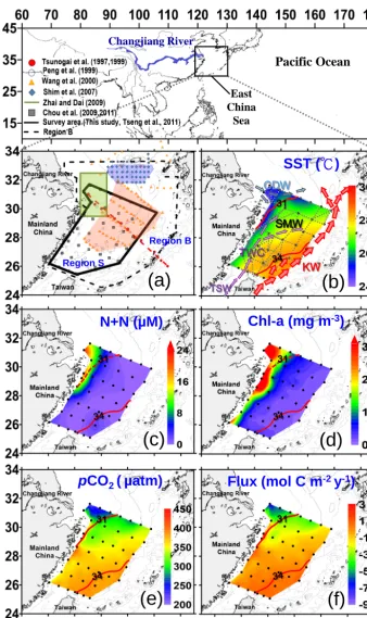
studies in the ECS with uptake rates of 1–3 mol C m−2yr−1 had been spatially limited as well (Fig. 1a). Moreover, a reli-able quantification in seasonally representative CO2uptakes

by the whole ECS has not been established to date.

The observational requirements to adequately investigate air–sea CO2exchange for the ECS are challenging due to the

high spatial and temporal heterogeneity and complexity of the physical and biogeochemical processes (Liu et al., 2003, 2010). Sea surface pCO2(pCO2w)distribution in the ECS

is spatially/temporally variable as a result of interactions be-tween the seasonal thermal cycle, net community production, surface/subsurface sea waters and river waters. The dominant processes in the ECS take place with typically active biolog-ical uptake of CO2in warm periods in the Changjiang plume

area. Although higher SST favors CO2 release to the

at-mosphere, better stratification favors phytoplankton growth, which draws down pCO2. However, while intense physical

mixing occurs in the cold season, the lower temperature in-creases the solubility of CO2 in the cold seasons that

over-compensates for the mixing up of CO2laden subsurface

wa-ter, usually resulting in a net air-to-sea CO2flux (Tseng et al.,

2011; Chou et al., 2011). In addition,pCO2wdistribution is

subjected to modification by mixing between different water masses, such as the nutrient-rich and less saline Changjiang Diluted Water (CDW, waters within 31 ‰ isohaline) and the warm, saline and nutrient-depleted waters, including the Kuroshio (KW), the Shelf Mixed (SMW) and the Taiwan Warm Current (TWC) waters (Fig. 1b). Consequently, the mixing of water masses with different biogeochemical char-acteristics in the ECS causes the spatial/temporal CO2

varia-tions (e.g., Tseng et al., 2011). Further, various circulation regimes lead to the shelf-edge processes for material ex-change between the East China Sea shelf and the shelf-break hugging Kuroshio (e.g., Liu et al., 2010). Thus, to enable bet-ter quantification of the ECS CO2uptake capacity reiterates

the need of greater spatial and temporal resolutions in ob-servational data, which are needed for accurate estimation of air–sea CO2fluxes in the ECS over an annual cycle.

This study presents new data and expands on the approach of Tseng et al. (2011) of adopting innovative methods to extend the spatial and temporal coverage for broad-scale assessments of distribution and air–sea exchange fluxes of CO2. A regional synthesis based on satellite remote sensing

data (e.g., sea surface temperature, SST) calibrated with di-rect near-surface underway pCO2 measurements and

mod-ified by the Changjiang (a.k.a Yangtze) River discharge

(CRD) has therefore been established. The CRD, as the dom-inant riverine nutrient source of the ECS, played a key influ-ence on modulating the CO2uptake (Tseng et al., 2011). We

found firstly an empirical relationship for predicting water

pCO2as a function of CRD and SST. The relation was then

applied to the whole ECS shelf (25–33.5◦N, 122–129◦E) af-ter the model generatedpCO2wresults had been well

vali-dated against the observedpCO2w. The resultant algorithm

aimed to improve the quantification of shelf CO2uptake

ca-pacity in the ECS eventually leads to a time series of the air–sea CO2exchange flux from 1998 to 2011 that yields an

annual mean value of unsurpassed accuracy after an exami-nation of different gas-transfer algorithms.

2 Materials and methods

2.1 Analytical methods and data analyses

Thirteen seasonal cruises for direct underway atmospheric (pCO2a)and waterpCO2(pCO2w)with hydrographic

mea-surements were carried out in the ECS shelf (25–32◦N, 120– 128◦E) between June 2003 and November 2011 on board R/V Ocean Researcher I. There was also one earlier cruise in July 1998 performing similar measurements. Most cruises (n=10) were conducted in warm seasons, whereas there were also cruises conducted in each of the other seasons (spring, fall and winter). Additional data were obtained to provide the complete seasonal coverage of CO2distribution

in the ECS. Although one-fourth of the cruises are during cold seasons, the limited cold-season data are accurate and coherent, and, therefore, representative. Essentially the cold season condition is controlled by cooling and vertical mix-ing, while the plume area is small. Therefore, the winter con-ditions are less variable in comparison to the warm season condition. In summer, by contrast, the conditions are mainly controlled by the Changjiang discharge, which is quite vari-able. Because the magnitude of the Changjiang plume in warm seasons determines the CO2uptake amount in the ECS

shelf (Tseng et al., 2011), it is necessary to conduct more cruises in summer to observe the conditions with high dis-charges of Changjiang. Consequently, the rich summer data allow us to delineate the effect of runoff variation on the bi-ological uptake of CO2.

The cruise tracks and hydrographic stations superimposed on main surface currents in this study area are shown in Fig. 1b. The underway system with continuous flow equili-bration, provided by the National Oceanic and Atmospheric Administration (NOAA) of the United States, is fully auto-mated and uses gas standards (thexCO2of the four standards

KW

TSW

CDW

SMW

TWC

31 Changjiang River

East China

Sea

Pacific Ocean

N+N (µM)

Chl-a (mg m

₎

31

31 31

31

pCO

(

µatm)

Flux (mol C m

_y

₎

Region B

Region S

SST (

℃

)

(a)

(b)

(c)

(e)

(f)

(d)

The precision and accuracy achieved with this method are ±0.1 and±1 µatm, respectively. The distributions of sea sur-face salinity (SSS) and temperature (SST) were recorded us-ing a SBE21 SEACAT thermosalinograph system (Sea-Bird Electronics Inc.). Surface chlorophyll a (Chla) concentra-tion was measured with a Sea Tech fluorometer attached to the Sea-Bird CTD (conductivity-temperature-depth) for a continuous in vivo fluorescence, with data calibrated by in vitro fluorometry (Turner Design 10-AU-005). Nutrient (e.g., nitrate + nitrite) and Chlaconcentrations were measured ac-cording to Gong et al. (1996) and Tseng et al. (2005).

The time-series records including remotely sensed SST data, archived hydrographic salinity (Japan Oceanographic Data Center, JODC), wind speed (at PenGaYi Islet; 25.62◦N, 122.07◦E), CRD (Datong hydrological gauge sta-tion; 30.76◦_{N, 117.62}◦_{E) and air pCO}

2 data (Jeju

Is-land, South Korea; 33.28◦_{N, 126.15}◦_{E) for estimating} pCO2w with related air–sea exchange flux in the ECS

re-gion (25–33.5◦N, 122–129◦E) were briefly described as below. The weekly average SST data were derived from the Advanced Very-High Resolution Radiometer (AVHRR) images from NOAA with 1 km×1 km resolution (http:// www.osdpd.noaa.gov/ml/ocean/sst.html). The AVHRR SST agreed well with shipboard observations (Tseng et al., 2007, 2009a, b). The archived hydrographic salinity data in the ECS were provided by the JODC with data resolution of 1◦×1◦ grids (http://jdoss1.jodc.go.jp/cgi-bin/1997/bss). The monthly wind speed data were estimated from the daily average data at the land-based weather station of Pen-GaYi Islet (25.62◦N, 122.07◦E) in the ECS provided by the Taiwan Central Weather Bureau (TCWB). The monthly CRD data at Datong hydrological gauge station (30.76◦_N,

117.62◦_{E) in the lower reach of Changjiang were obtained}

from the Hydrological information Centre of China (http:// sqqx.hydroinfo.gov.cn/websq/). The airpCO2was estimated

from the monthly atmospheric xCO2 (mole fraction)

mea-sured at Jeju Island (South Korea; 33.28◦N, 126.15◦E), after correction for water vapor pressure at 100 % humidity with SST and salinity data (http://www.esrl.noaa.gov/gmd/ccgg/ globalview/).

2.2 Air–sea CO2exchange flux estimates

Air–sea exchange flux, F, ofpCO2is estimated using the

equation F=K×δpCO2, where K (gas transfer

coeffi-cient) =kL(k: transfer velocity; L: gas solubility),δpCO2

is the difference between the pCO2 of surface water and

air (i.e.,pCO2w−pCO2a). ThepCO2awas estimated from

the monthly average pCO2 observed at Jeju Island during

the study period. Solubility of CO2 as a function of water

temperature and salinity can be estimated from the Weiss (1974) empirical equation. To obtain a more representative flux, gas transfer velocity (k) is derived using the Wan-ninkhof (1992, short-term formula) empirical relationship:

k=0.31×u2×(Sc/660)−0.5, where the Schmidt number

(Sc) is temperature-dependant for CO2 in seawater,

com-puted from in situ temperature data anduis the wind speed at 10 m height obtained from PenGaYi station (monthly aver-age wind data from the TCWB database of 1998–2011). The parameterization of Wanninkhof (1992), representing a rea-sonable estimate for calculating wind-inducedk, was firstly used for comparison with previous flux estimates in the ECS. Then, the air–sea exchange fluxes of CO2 in the ECS

re-ported in the previous studies were re-calculated according to the consistent wind speed data and Wanninkhof’s algorithm used in this study. Finally, uncertainties of CO2fluxes due to

using different gas-transfer algorithms (e.g., Liss and Mer-livat, 1986; Wanninkhof, 1992; Wanninkhof and McGillis, 1999; Jacobs et al., 1999; Nightingale et al., 2000; McGillis et al., 2004; Ho et al., 2006; Wanninkhof et al., 2009) and their appropriate flux ranges in the ECS shelf were quantita-tively evaluated.

2.3 Areal mean ofpCO2and environmental variables

To obtain a representative mean value for the ECS shelf, we prepared the interpolated data set of 0.01◦×0.01◦ (about 1 km×1 km grid points from observedpCO2and other

en-vironmental variables (e.g., SST, SSS, N + N, Chla etc.) by kriging and then calculated the areal means by integrating over the survey area. The grid resolution matches the spatial resolution of weekly AVHRR-SST data. For the areal mean of the air–sea flux, we first calculated the flux within a given grid box along the cruise track for underwaypCO2

measure-ments using the average values of SST, salinity, andδpCO2

in the box and the monthly averaged wind speed; then, we calculated the areal mean CO2flux over the study area in the

same fashion mentioned above. Likewise, we computed the monthly flux estimates for the model study regions, encom-passing almost the entire ECS (i.e., Region B: 25–33.5◦N, 122–129◦E, Fig. 1a), from the modeled averagepCO2which

was generated on a monthly basis from the CRD and SST.

3 Results and discussion

3.1 Representativeness of the study region

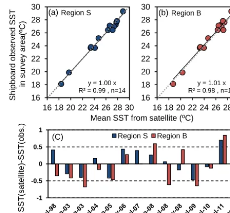
observed values in cruise survey area correlated well with the average AVHRR-SST data in two model domains with per-fect regression relationships (R2≥0.98) as shown respec-tively in Fig. 2a and b. It indicates, on the one hand, the re-motely sensed SST data used here are reliable and validated in terms of data assurance. After calibration, the satellite SST data have overall averaged RMSEs (root mean square errors) of less than 0.5◦C (e.g., 0.37 and 0.49◦C in Regions S and B, respectively) (Fig. 2c). In the East China Sea, the dif-ferences in SST between adjacent months are, on average, about 2.3◦, which is much greater than the possible errors in satellite SST. It demonstrates that errors in the remotely sensed SST do not affect significantly the calculation of the monthly variability in CO2solubility. On the other hand, the

areal mean SST data obtained on our cruise investigations can represent the variability of the areal mean value of the entire ECS. Therefore, it is reasonable to assume that the re-lationship between the areal means ofpCO2and mean

val-ues of hydrographic variables obtained on our cruises was also representative for the entire ECS.

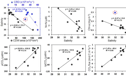
The average SSS is also representative. In the river-influenced ECS shelf, most variables are strongly controlled by mixing, i.e., well correlated with SSS (Fig. 3; Tseng et al., 2011). The relationships were mostly a reflection of mix-ing between the Changjiang runoff and the open shelf waters (e.g., Kuroshio or TWC waters). A very good correlation be-tween the average salinity and CRD was obtained. It is noted that a good correlation was also found between the average SSS and the area of the CDW (defined asS <31). So, we can see the salinity as a proxy of CDW or vice versa. Drawdown of CO2occurs in the mixing zone in the open shelf, where the

biological pump kicks in. The concurrent mixing and biolog-ical processes are responsible for the observed correlations. The areal mean SSS in Regions S and B are rather similar and both are representative. Briefly, the Changjiang River plume is the most important feature in the CO2uptake processes in

the warm season, and has been well observed on our cruises, i.e., most of it has been captured in observations. As a first approximation, the peripheral regions to the north and south of the plume are more or less symmetric and, therefore, the southern shelf is representative of the whole ECS shelf. Fur-ther, we may use the aforementioned relationship to derive representative average values ofpCO2for Region B, which

should be the most representative for the ECS shelf. 3.2 Summer CO2uptake determined by Changjiang

river discharge

Figure 1e and f show the composite distributions ofpCO2w

and air–sea CO2 exchange flux from nine cruises in

sum-mer between 2003 and 2011 (see Fig. S1 for the underway measuredpCO2along with cruise track). As reported

previ-ously and shown in Fig. 1, thepCO2wdistribution in the ECS

was associated with variations of water masses (Tseng et al., 2011). LowerpCO2wvalues were observed in the CDW

y = 1.00 x R² = 0.99 , n=14

16 18 20 22 24 26 28 30

16 18 20 22 24 26 28 30 Region S

y = 1.01 x R² = 0.98 , n=14

16 18 20 22 24 26 28 30

16 18 20 22 24 26 28 30

-1 -0.5 0 0.5 1

Region S Region B (C) S hi pboar d obs er v ed SST i n s ur v ey ar ea (º C)

Mean SST from satellite (ºC)

(a) (b) Region B

SST (s a te lli te )-SST (o b s .)

Figure 2. Linear regression relationships between areal mean AVHRR SST in two model regions, i.e., (a) S and (b) B; and field observed areal mean SST in cruise survey area (dashed line is 1:1 reference line). (c) Differences between the calibrated satellite data and shipboard-observed SST from 1998 to 2011.

plume area near the Changjiang River mouth and higher val-ues in the southeastern shelf area, where saline and nutrient-depleted Kuroshio, Shelf Mixed Water and Taiwan Warm Current water prevailed. Also, the distribution of CO2flux in

the ECS resembled that ofpCO2. More negative values (i.e.,

uptake of atmospheric CO2 by surface water) were mostly

found in the nutrient-rich river plume area with a gradual increase to the east and south. Despite the high sea surface temperature in summer that favored release of CO2 to the

atmosphere, the Changjiang River plume acted as a strong CO2 sink, mainly due to CO2drawdown in the outflow

re-gion where riverine nutrients induced strong phytoplankton growth, resulting in high Chlaand reducedpCO2in the

sur-face layer (Tseng et al., 2011).

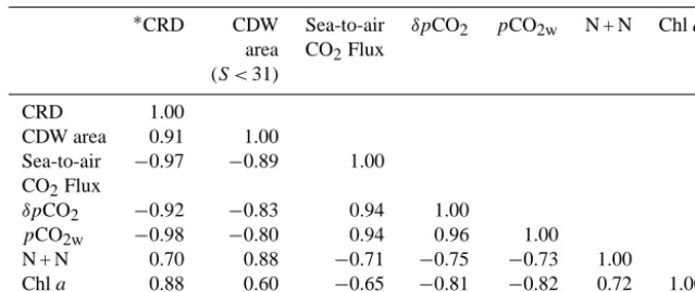
The results obtained through the statistic correlation analy-ses (Table 1) and figures (Figs. 3, 4) for areal means ofpCO2

and other environmental variables further demonstrate that the biological sequestration of CO2in the warm periods, as

indicated by the relatively low summerpCO2, was well

cor-related to the CRD. Figure 4 also illustrates that the whole ECS CO2uptake was significantly correlated with the CDW

area, the Changjiang discharge, the amounts of N + N or the mean Chla in summer. The relationship between CO2

up-take and nutrients suggest that the observed nutrient concen-tration supported the DIC (dissolved inorganic carbon) up-take, even when the surface was warming and favored CO2

Table 1. Correlation coefficient matrix for areal means ofpCO₂and other environmental variables in the ECS shelf in summer months from 1998 to 2011 (n=10).

∗_{CRD CDW Sea-to-air δpCO}

2 pCO2w N + N Chla area CO₂Flux

(S <31)

CRD 1.00

CDW area 0.91 1.00

Sea-to-air −0.97 −0.89 1.00 CO2Flux

δpCO2 −0.92 −0.83 0.94 1.00

pCO2w −0.98 −0.80 0.94 0.96 1.00

N + N 0.70 0.88 −0.71 −0.75 −0.73 1.00

Chla 0.88 0.60 −0.65 −0.81 −0.82 0.72 1.00

∗_{Average Changjiang River discharge data collected at Datong station during the LORECS cruise period.}

Regression results between other variables and Changjiang discharge were obtained for the ten cruises, not including OR1-686 (19–26 June 2003). Before that cruise, the Typhoon Soudelor (16–18 June 2003) passed over east of the ECS shelf toward Korea and Japan. Such a typhoon effect anomalously induced the more diluted plume area through enhanced rainfall in the lower watershed of Changjiang below Datong station. However, high typhoon-induced discharge was not recorded at Datong which is 624 km upstream from the river mouth.

amount of CO2 taken up by the sea in July or during the

warm period are between 5 and 7, which agrees well with the Redfield ratio. The preliminary results show that the nu-trient fluxes (July: nitrate, 9.9 Gmol under averaged CRD 45 000 m3s−1; warm periods: 51 Gmol under 39 000 m3s−1)

discharged to the sea were enough to support the DIC uptake estimated by air–sea exchange (July: 44 Gmol under the up-take rate of 0.88 mol C m2yr−1; warm period: 360 Gmol un-der 1.21 mol C m2yr−1). Please note that near-shore areas in the low salinity zone of the Changjiang plume with strong respiration (Zhai et al., 2009) and the coastal upwelling zone (Chou et al., 2009) had highpCO2values. However, the

out-gassing areas (<4 % of the ECS shelf area) were very small relative to the CO2uptake areas in the open shelf based on

the weighted statistic analyses. It barely changes the net sink terms at all. Consequently, the CO2distribution/uptake

dy-namics were associated yearly with the changes of the plume expansion determined by the CRD:

pCO2= −3.9×CRD+517, R2=0.97, n=9; (1)

CO2flux= −0.19×CRD+7, R2=0.95, n=9. (2)

where CRD is in units of 103m3s−1. The results demonstrate again that Changjiang River discharge governs coastal ocean production and CO2uptake capacity in the East China Sea

shelf in summer.

3.3 Empirical algorithm to simulate seasonalpCO2w variations

To derive representative mean values ofpCO2win different

seasons in the entire ECS shelf, we may use the strong cor-relation between river discharge and CO2uptake mentioned

above (e.g., Tseng et al., 2011). We thus developed an em-pirical algorithm by using the monthly areal mean (referred

to as “average” hereafter) of observedpCO2w, SST and the

CRD during warm periods. The data mentioned above were collected during warm cruises between May and Novem-ber between 1998 and 2011. Firstly, we found normalized

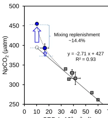
pCO2at 25◦C (NpCO2)correlated negatively with the CRD

(×103m3s−1)with a good regression relationship (Fig. 5) as follows:

NpCO2at 25◦C= −2.71×CRD+427 (R2=0.93). (3)

Here, NpCO2 at 25◦C, which is the observed average pCO2wnormalized to a constant temperature of 25◦C (mean

SST of all cruises), was computed by using the following equation proposed by Takahashi et al. (1993):

NpCO2atTmean=(pCO2w)obs×exp[0.0423(Tmean−Tobs)],

(4) whereTmeanis 25◦C andTobsis the observed monthly mean

value and (pCO2w)obsis the observed averagepCO2w. The

purpose of “pCO2normalized to 25◦C” is to eliminate the

temperature effect in order to discern other factors (e.g., bi-ological activities, air–sea exchange and vertical transport of subsurface waters etc.) that affectpCO2.

The inversely linear relationship between the NpCO2and

CRD during warm periods as shown by Eq. (1) indicates that

pCO2w changes in the ECS shelf water were mainly

gov-erned by biological processes, while other processes, such as the upward transport of DIC from subsurface waters and the air–sea CO2exchange, are minimal under strong

stratifica-tion.

We finally refined the empirical algorithm for predicting

pCO2waccording to Eqs. (3) and (4) as below,

Figure 3. Relationships between areal mean SSS and hydrographic variables in the whole ECS. (*A triangle denotes the data obtained from the cruise of OR1-686 (19–26 June 2003). In the plot of Chlavs. salinity, the circled triangle is an outlier that was not included in the regression analysis. The outlier was probably caused by the Typhoon Soudelor (16–18 June 2003) that passed over the eastern ECS shelf right before the cruise. The anomalously low salinity was probably caused by the typhoon rain instead of the river discharge, while the high Chlalevel was probably caused by typhoon-driven vertical mixing rather than river discharged nutrients.

where−2.71 is the slope obtained from the plot of NpCO2

versus CRD; CRD is the Changjiang River discharge in units of 103m3s−1;Tobsis the monthly average AVHRR SST. As

mentioned above, thepCO2estimates should be reasonable

since the bias in AVHRR SST has been minimized (lower than 0.5◦C; an estimated error of<10 µatm; Fig. 2c).

However, when we applied the same relationship to the cold season, we found that the relationship underestimated the NpCO2 (Fig. 3). The extra increment was probably

mainly caused by the increase in DIC provided by enhanced vertical mixing in the cold season. It is necessary to com-pensate for the mixing effect in the equation. As shown in Fig. 3, an increase of 57.4 µatm was needed to reach the observed NpCO2 of 455.1 µatm for January from the

com-puted NpCO2of 397.7 µatm, which was calculated from the

CRD of 10 211 m3s−1. This increment represents a 14.4 % increase to account for the mixing replenishment.

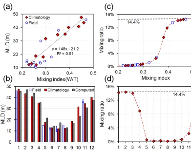
For the model calculation, the seasonal mixing contri-bution could be estimated from the data of wind speed (W) and remotely sensed SST (T) through the relation-ship between the mixing ratio and the mixing index de-fined asW/T (Fig. 6). We firstly found a significant correla-tion between climatological monthly averaged mixed layer depth (MLD) data obtained from the Ifremer/Los Mixed Layer Depth Climatology website (http://www.ifremer.fr/ cerweb/deboyer/mld/Surface_Mixed_Layer_Depth.php) and

Figure 4. Relationships betweenδpCO2and (a) the CDW plume area or the CRD; and (b) N + N and Chlain summer from July 1998 to July 2011 in the ECS shelf. “−“ indicates uptake of CO2 by shelf water from the atmosphere. The best-fit lines by a linear regression analysis (n=10, allpvalues<0.001) are shown in the plume area and Chla(solid line) and in CRD and N+N (dashed line), respectively. The CRD denotes average Changjiang River dis-charge data collected at Datong station during the LORECS cruise period. The blue circled triangle denotes the data point from the OR1-686 cruise, which was excluded from the regression analysis.

y = -2.71 x + 427 R² = 0.93

250 300 350 400 450 500

0 10 20 30 40 50 60 70

N

p

C

O2

(

μ

a

tm

)

CRD ( x103 _m3 _s-1₎

Mixing replenishment ~14.4%

Figure 5. The correlation between monthly average NpCO2and CRD (black square) was observed during warm cruises from May to November between 1998 and 2011: observed NpCO2 about 455.1 µatm (blue dot) and the computed NpCO2397.7 µatm (dotted circle) at the CRD at 10 211 m3s−1during the January cruise.

correlates to W and negatively toT, i.e., MLD∞W/T as the mixing index. Further, the computed MLDs estimated by the MLD–W/T relationship are in excellent agreement with observations and climatologic averages (Fig. 6b). It indicates the mixing index as wind versus SST (W/T) shall be con-sidered as a proper vertical mixing parameter. The seasonal mixing ratio as a function of mixing index further follows an arctan curve made by the inverse tangent function: mix-ing ratio (%) = (tan−1[61.2(W/T )−23] +1.5)/20 (Fig. 6c). Overall, the greatest contribution of the mixing replenish-ment is ca. 14.4 % due to strongly vertical mixing in cold months (e.g., January, February and March) in the ECS shelf, when the SST is the lowest and wind speed highest during the northeast monsoon (Fig. 6d). During warm periods, the con-tribution of the mixing tends to almost zero due to a strong stratification. A distinctly seasonal change in mixing contri-bution will occur during the monsoon transition/season, al-ternating from the cold to the warm periods or vice versa. 3.4 Time series of model results vs. field observations

Tseng et al. (2011) demonstrated the Changjiang plume size is directly governed by the Changjiang River discharge (Table 1; Fig. 3a). Intraseasonal variations in plume area were hence observed due to intraseasonal changes in the Changjiang River discharge. Additionally, both waterpCO2

and NpCO2during the warm period were all well correlated

with Changjiang River discharge (Figs. 3, 4). The discharge, which governs the nutrient inputs into the ECS, is the pri-mary factor to control the CO2 uptake of the whole ECS.

In summary, the focus on NpCO2during the productive

pe-riod in summer is bound to emphasize the river’s effect (i.e., high river discharge, causing high nutrient inputs and induc-ing phytoplankton growth) on biological export. Therefore, although we conducted only one cruise between 1998 and 2002, the general feature of the river effect on the CO2

up-take in the river-dominated ECS system should be applicable. The 14-year time series of model results of monthly mean

pCO2w,δpCO2and the air–sea CO2 flux in Regions S and

B over the study period (1998–2011) are shown in Fig. 7, in which mean observed values of the 14 cruises are also plotted for comparison. It is clear that all modeledpCO2w, δpCO2 and the CO2 flux agree well with the observations

(Fig. 7; Supplement Fig. S2). The good linear relationships between the modeled areal means and the means of observed values confirm the satisfactory performance of the empiri-cal algorithm, which has been applied to both the small and big domains (S and B) of the ECS (Supplement Fig. S2). The uncertainty resulting from parameterization of the mean

pCO2may be indicated by the root mean square of the

de-viations between the model results and observations, which was found to be 13.4 µatm (n=14). It is noted that the mean deviation, 0.7 µatm, was quite small.

As shown in Fig. 7b, the time series is characterized by a distinct seasonal pattern with a maximum in late summer– mid-fall and a minimum in spring. In general, thepCO2w

mostly remained belowpCO2a throughout an annual cycle

except during the period from late summer to mid-fall. That means the evasion of CO2occurred primarily in a relatively

short period in the warm season. Moreover, the amount of CO2released was small relative to the drawdown of CO2in

other seasons. TheδpCO2, which represents a driving

po-tential for CO2 gas transfer across the water–air interface,

seasonally fluctuated with a slight supersaturation of about +10 µatm, signifying a source of CO2, from the ECS to

atmo-sphere, on average in late summer to mid-fall and a strong un-dersaturation of−80 µatm, signifying a sink of atmospheric CO2, in spring (Fig. 7c).

There were also apparent interannual variations, which showed unusually high peak values in 2001, 2006 and 2011 (drought years) and exceptionally low values in 1998 and 2010 (flood years). There were anomalously strong super-saturations observed in the late summers of 2001, 2006 and 2011 and undersaturation in the summer of 1998 and late spring of 2010, respectively, due to the Changjiang discharge fluctuations caused by climate change (Tseng et al., 2011). Subtle long-term increasing trends in pCO2a and pCO2w

were distinctly observed:

pCO2a=1.9(±0.0)×t+353.4(±0.2), r2=0.99, n=14; (6) pCO2w=2.1(±0.8)×t+309.5(±6.8), r2=0.36, n=14, (7)

wheret= year−1997. ThepCO2ahas been increasing from

Figure 6. (a) Relationship between averaged MLD obtained from monthly climatology and field observations and mixing index (W/T). (b) Comparison of the computed MLD with those from climatology and field. (c) Arctangent relationship between the mixing index and contribution ratio. Blue dot: field surveys; red diamond: climatology monthly averages. (d) Monthly variability in the contribution ratio of vertical mixing in the ECS.

pCO2aseasonality shows a spring high and a summer low.

Please note the atmosphericpCO2observed from the cruise

correlated well with the time-series data measured at Jeju Is-land (fieldpCO2a (LORECS) = 1.01×pCO2a(Jeju),R2=

0.90, n=13; Fig. 7b). The rate of increase in pCO2w of

about 2.1 µatm yr−1 was slightly higher than that inpCO2a

during the study period so that δpCO2 results showed an

increase at a rate of 0.2 µatm yr−1. The increasing δpCO2

can in part be due to decreasing CRD under environmen-tal changes, e.g., the operation of Three Gorges Dam and the water transferring scheme from south to north in China (Tseng et al., 2011). Eventually, if this trend is true and it continues, the uptake in the ECS will gradually decrease.

The surfacepCO2wandδpCO2(summarized in Table 2)

varied seasonally and interannually in the ECS shelf. The annual pattern in δpCO2 shows that negative δpCO2

oc-curs in the whole year. Overall, the ECS shelf serves as a net sink of atmospheric CO2with−38±13 µatm ofδpCO2

on average, with a strong sink in winter (−43±12 µatm) and spring (−75±12 µatm), and a weak sink in summer (−28±33 µatm) and fall (−6±15 µatm). Data from a few other cruises (spring, fall and winter) will also be used to

show the complete seasonal CO2distribution in this region

(Fig. 7c; Table 3). The average annual δpCO2 was

calcu-lated to be about −46±45 µatm with the seasonal vari-ability at ca. −109, −25±39 (n=3), −6, and −46 µatm for spring, summer, fall, and winter, which were consistent with those estimated by model. The seasonal pattern shows a sink-to-source transition in late summer–mid-fall during the Changjiang River plume reduction after the July maxi-mum discharge (see Fig. 9; Tseng et al., 2011). Furthermore, the weak sink status during warm periods is fairly sensitive to changes of pCO2 and to become a CO2 source due to

the Changjiang discharge decreases through environmental changes (Tseng et al., 2011).

3.5 Comparison with previous estimates

Figure 8 further shows the comparison of δpCO2, in the

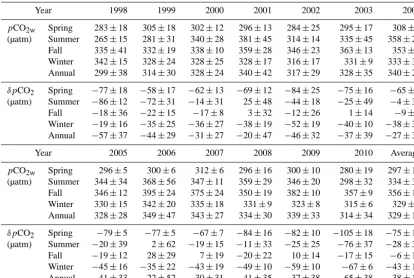
Table 2. The seasonal and annual average CO₂results between 1998 and 2010 in the ECS shelf.

Year 1998 1999 2000 2001 2002 2003 2004

pCO2w Spring 283±18 305±18 302±12 296±13 284±25 295±17 308±6 (µatm) Summer 265±15 281±31 340±28 381±45 314±14 335±45 358±27 Fall 335±41 332±19 338±10 359±28 346±23 363±13 353±5 Winter 342±15 328±24 328±25 328±17 316±17 331±9 333±34 Annual 299±38 314±30 328±24 340±42 317±29 328±35 340±26

δpCO2 Spring −77±18 −58±17 −62±13 −69±12 −84±25 −75±16 −65±7 (µatm) Summer −86±12 −72±31 −14±31 25±48 −44±18 −25±49 −4±31 Fall −18±36 −22±15 −17±8 3±32 −12±26 1±14 −9±7 Winter −19±16 −35±25 −36±27 −38±19 −52±19 −40±10 −38±36 Annual −57±37 −44±29 −31±27 −20±47 −46±32 −37±39 −27±31

Year 2005 2006 2007 2008 2009 2010 Average

pCO2w Spring 296±5 300±6 312±6 296±16 300±10 280±19 297±10 (µatm) Summer 344±34 368±56 347±11 359±29 346±20 298±32 334±34 Fall 346±12 395±24 375±24 350±19 382±10 357±9 356±19 Winter 330±15 342±20 335±18 331±9 323±8 315±6 329±8 Annual 328±28 349±47 343±27 334±30 339±33 314±34 329±14

δpCO2 Spring −79±5 −77±5 −67±7 −84±16 −82±10 −105±18 −75±12 (µatm) Summer −20±39 2±62 −19±15 −11±33 −25±25 −76±37 −28±33 Fall −19±12 28±29 7±19 −20±22 10±14 −17±15 −6±15 Winter −45±16 −35±22 −43±19 −49±10 −59±10 −67±6 −43±12 Annual −41±33 −22±52 −30±31 −41±35 −37±38 −65±38 −38±13

short-term formula). In addition, the Changjiang discharges in reported references were plotted in the discharge range of the climatological monthly mean with±1 standard deviation (SD; 1998–2010) as a reference level to check anomalous events (Fig. 9a). The results show there were three flood surveys obtained in July 1992, 1998 and 2010 and others mostly fell within±1 SD range of the climatological mean. As a whole, most of the publishedpCO2values are erratic

away from 1:1 reference line outlier levels of ±20 µatm (e.g., Peng et al., 1999; Wang et al., 2000; Shim et al., 2007; Zhai et al., 2009) while some are close to model outputs (e.g., Tsunogai et al., 1999; Wang et al., 2000, in summer; Chou et al., 2011; this study). The estimates with large uncertainties are mainly due to inadequate representativeness of the spatial variability and limited sampling resolution. These problems in each report are briefly summarized in the remarks in Table 3 and the following text.

Tsunogai and coworkers (1997, 1999), for instance, re-ported the air–sea exchange fluxes of CO2in the whole ECS

were only extrapolated from a single transect data set of the PN line across the northern ECS (Fig. 1a; Table 3). There-fore, the findings in summer and winter applied to the whole ECS from one survey line certainly cause biases and slightly higher values than the model ones (Fig. 9b, c). Their de-veloped algorithm was not suitable for the use of the near-shore waters. Likewise, thepCO2data of Peng et al. (1999)

were all generated from the TA and TCO2which were only

collected in spring and limited in low-resolution samplings.

Moreover, the study area of Peng et al. (1999) was mostly located in the Kuroshio, Mixed Shelf and Taiwan Warm Current waters and lacked coverage of coastal plume wa-ters. Higher results in spring than those by the model were therefore found (Fig. 9b, c), since coastal plume processes which drew the CO2low via phytoplankton blooms near the

Changjiang River mouth were not observed.

Wang et al. (2000) had only two field observations in spring and summer, while their fall and winter data were computed from Tsunogai’s empirical algorithm. Their obser-vations lacked data from the coastal waters, although they had a wide-area survey (Fig. 1a). Hence, the springpCO2

data in the whole ECS, being derived from a temperature-dependent relationship, were higher than those by the model, which could not reflect the biological uptake by plankton blooms in the Changjiang plume (Fig. 9b, c). The summer results derived from the salinity relationship were lower than the modeled ones. That was because of lack of the data from additional replenishment of CO2from subsurface waters by

coastal upwelling. Additionally, the fall and winter data de-rived from Tsunogai’s algorithm could not reflect the addi-tional CO2by vertical mixing during the cold seasons.

There-fore, those data generated from Tsunogai’s algorithm were lower than our data by model and field observation (Fig. 9b, c).

The study in Zhai and Dai (2009) was focused on the ar-eas near the Changjiang estuary so that thepCO2 data had

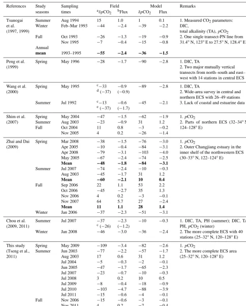
Table 3. Summary of the CO₂results in the ECS reported in the previous studies and obtained from this study.

References Study Sampling Field Model Remarks

seasons times aδpCO₂ bFlux δpCO₂ Flux

Tsunogai et al. (1997, 1999) Summer Winter Aug 1994 Feb–Mar 1993 15 −44 1.0 −2.4 1 −39 0.1 −2.2

1. Measured CO₂parameters:

DIC,

total alkalinity (TA),pCO₂

Fall Oct 1993

Nov 1995 −26 −7 −1.3 −0.4 −19 −15 −0.9 −0.8

2. One single transect-PN line from

31.4◦N, 123◦E to 27.5◦N, 128.4◦E

Annual

mean 1993–1995 −55 −2.4 −36 −1.5

Peng et al. (1999)

Spring May 1996 −28 −1.7 −90 −2.8 1. DIC, TA

2. Two major mutually vertical transects from north–south and east– west with 14 stations in central ECS

Wang et al. (2000)

Spring May 1995 c−33

d₍₋₃₇₎

−0.9

(−0.9)

−89 −2.8 1. DIC, TA

2. Wide-area survey in central and northern ECS with 26–49 stations

Summer Jul 1992 c−13

e₍₋₃₇₎

−0.6

(−1.7)

−45 −2.1 3. Lack of coastal and estuarine data

Shim et al. (2007) Spring Summer Fall May 2004 Aug 2003 Oct 2004 Nov 2005 −47 −23 11 4 −1.5 −0.9 0.8 0.2 −62 31 −3 −26 −1.9 1.2 −0.2 −1.4

1.pCO₂

2. Parts of northern ECS (32–34◦N,

124–128◦E)

Zhai and Dai (2009)

Spring Mar 2008

Apr 2005 Apr 2008 May 2005 Mean −38 −10 −79 −67 −48 −1.5 −0.4 −3.1 −2.4 −1.8 −76 −84 −103 −74 −84 −3.0 −3.1 −4.0 −2.5 −3.1

1.pCO₂

2. Outer Changjiang estuary in the inner shelf of the northwestern ECS

(30–33◦N, 122–124◦E)

Summer Jul 2007

Aug 2003 Mean −74 −45 −60 −2.4 −1.7 −2.1 −10 31 10 −0.3 1.2 0.4

Fall Sep 2006

Oct 2006 Nov 2006 Nov 2007 Mean 22 −45 4 64 11 1.1 −2.7 0.2 5.7 1.1 53 35 −3 27 28 2.2 1.3 −0.1 −2.4 1.4

Winter Jan 2006 −37 −2.3 −51 −3.1

Chou et al. (2009, 2011)

Summer Jul 2007 −37

c₍₋₂₆₎

−2.3

(−1.2)

−10 −0.3 1. DIC, TA, PH (summer); DIC, TA,

PH,pCO₂(winter)

Winter Jan 2008 −46 −3.0 −36 −2.4 2. The more complete ECS with 40

stations (25–32◦N, 120–128◦E)

This study (Tseng et al., 2011) Spring Summer May 2009 Jun 2003 Aug 2003 Jul 2004 Jun 2005 Jul 2007 Jul 2008 Jul 2009 Jul 2010 Jul 2011 −109 −77 17 −5 −47 −23 3 −8 −103 −15 −3.4 −2.2 0.6 −0.3 −1.7 −0.7 0.2 −0.4 −4.7 −0.6 −82 −57 31 −2 −65 −10 10 −18 −88 −4 −2.6 −1.7 1.2 −0.1 −2.3 −0.3 0.5 −0.9 −3.9 −0.1

1.pCO₂

2. The more complete ECS area

(25–32◦N, 120–128◦E)

Fall Nov 2006

Nov 2011 −15 4 −0.6 0.2 −3 −7 −0.1 −0.4

Winter Jan 2008 −46 −3.0 −36 −2.4

a_{Units inδpCO}

2and CO2flux are µatm and mol C m−2yr−1, respectively;

b_{Recalculated by wind speed data at PenGaYi and Wanninkhof’s gas transfer algorithm (1992, short-term formula);} c_{Average of all stations;}

d_{Averaged by values derived frompCO}

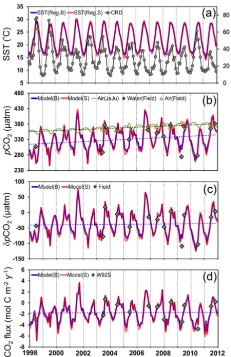
Figure 7. Time-series variations (model results with observed data of 14 cruises) in monthly areal mean (a) SST and CRD, (b)pCO2w and pCO2a, (c) δpCO2, and (d) CO2 flux in the sea surface of the ECS shelf (“+”: sea to air; “−“: air to sea) between 1998 and 2011. The tick on the time axis corresponds to 1 January of the year marked.

with plume dynamics (Fig. 8). Low summer data were, for example, observed due to a strong bio-uptake of CO2

rela-tive to data for the whole ECS, while highpCO2in fall was

due to a strong vertical mixing (Fig. 9b, c). The data of Shim et al. (2007) which were collected in the northeastern ECS is lower in summer and higher in spring, fall and winter than model ones (Fig. 9b, c). That might be attributed to more dispersion of the Changjiang plume to the northeast of the ECS in summer, at the period of drawdown, and the more intensive vertical mixing induced by the colder SST in cold seasons to bring the more enriched-CO2subsurface water to

the surface, respectively. The comparison results further in-dicate small-scale spatial surveys which were performed in the Changjiang estuary and northern ECS area could not be representative of the whole ECS shelf.

-120 -100 -80 -60 -40 -20 0 20 40 60 80 100

-120 -100 -80 -60 -40 -20 0 20 40 60 80 100

δ

p

C

O2

(

li

te

ra

ture

)

δ pCO2 (model)

Tsunogai et al. (1997,1999) Peng et al. (1999) Wang et al. (2000) Shim et al. (2007) Zhai and Dai (2009) Chou et al. (2009,2011) This study

1:1 ±20 µatm

Figure 8.δpCO2comparison between the data retrieved from pub-lished references and this study and those generated by the model at the same surveying time.

Chou et al. (2011) covered the more extensive areas like our study area so that the areal mean fluxes were rather con-sistent with ours. After all, the outputs from our algorithm were validated by our field observations of in situ underway

pCO2with high spatial and temporal resolutions since 2003

(Fig. 7b, c, d). The modelpCO2w results agreed well with

the observedpCO2w (R2=0.90,n=14; Fig. 7b). In

addi-tion, our algorithm can reflect the results caused by anoma-lous flood events, e.g., the floods of July in 1998 and 2010 causing exceptionally lowpCO2wvalues and high CO2

up-takes (Table2; Fig. 9a, b, c). Therefore, this assessment of an-nual CO2uptake is more credible than all previous estimates

(1–3 mol C m−2yr−1)since our better spatial and temporal coverage reduces uncertainties.

3.6 Comparison with flux estimates by different gas-exchange algorithms

Factors that affect air–sea CO2 flux estimates using the

two-layer gas exchange model are mainly from two parts: (1) environmental forcing factors that control the gas trans-fer velocity,k (m s−1), and (2) thermodynamic driving po-tentials that affect air–sea pCO2 concentration differences

Month

Spring Summer Fall Winter

δ

p

CO

2

(µ

at

m

)

C

O2

f

lu

x

(

mo

l

C

m

-2 y -1)

C

RD

(

x10

3 m 3 s

-1)

(a)

(c)

(b)

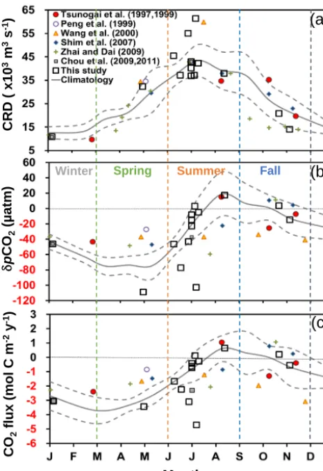
Figure 9. Seasonal monthly patterns revealed in observational data of (a) CRD, (b) δpCO₂and (c) air–sea CO₂flux, obtained from published references and from field data in this study and model results. The thick curves denote the climatological mean and the dashed curves denote the range of ±1 SD during the study period of 1998–2011.

and McGillis, 1999 (WM99: WM99S; WM99L); Jacobs et al., 1999 (J99); Nightingale et al., 2000 (N00); McGillis et al., 2004 (M04); Ho et al., 2006 (H06); Wanninkhof et al., 2009 (W09)). The plot of different algorithms fork against wind speed, as shown in Fig. 10, reveals that the differ-ences among the algorithms significantly increase with in-creasing wind speed, i.e., at low wind speeds they are much less than those at high wind speeds (>10 m s−1). In this study, the monthly average wind speed obtained from Pen-GaYi station in the ECS ranged between 5 and 11 m s−1_with

stronger winds in cold seasons during the northeast mon-soon (Fig. 10). Varying up to almost threefold of differences among different algorithms for the calculation, the wind-inducedkwas calculated to be the highest by J99 and lowest by LM86. It further demonstrates the largest source of uncer-tainties involved in estimating air–sea CO2flux resides with

these algorithms. Particularly, the differences would increase drastically among the models developed by J99, W92L and

0 10 20 30 40 50 60 70 80

4 5 6 7 8 9 10 11

k

(c

m

h

r

-1

)

Wind Speed (m sec

₎

W92L J99 WM99L W92S N00 M04 H06 LM86 WM99S W09

Min.

Mean

Max.

Figure 10. Comparison among different algorithms for flux calcu-lation against wind speed (LM86 corresponds to Liss and Merlivat (1986); other labels see in Table 4). Black dashed lines in min, mean and max denote the minimum, average and maximum monthly aver-age wind speeds obtained from PenGaYi station in the ECS during the study period.

0.0 1.0 2.0 3.0 4.0 5.0

A

nnua

l C

O2

f

lu

x

(

m

o

l m

-2 y -1)

Overall avg:1.7 ± 0.6

(I): 2.5 ± 0.5 (II): 1.5 ± 0.2 (III): 1.2 ± 0.1

Figure 11. Comparison among the averaged annual CO2fluxes esti-mated by different algorithms in the study period. Three distinctive groups: (I) highest average:−2.5±0.5 mol C m−2yr−1; (II) mid-range:−1.5±0.2; (III) low values:−1.2±0.1 with an overall av-erage:−1.7±0.6.

WM99L when the wind speed increases, while the algorithm developed by N00, M04 and H06 would not differ substan-tially, as compared to W92S (Fig. 10).

In Table 4, the summary of the averaged seasonal and annual CO2 fluxes between 1998 and 2010 is shown for

comparison, calculated from the above-mentioned 10 al-gorithms by using monthly wind speed data measured at PenGaYi station. Overall, the averaged annual CO2 fluxes

Table 4. Seasonal average CO2fluxes between 1998 and 2010 derived from the reported gas-transfer algorithms∗.

Seasons LM86∗ W92L W92S WM99L WM99S J99 N00 M04

Spring −3.0±0.4 −4.6±0.7 −3.7±0.5 −4.5±0.7 −2.3±0.4 −6.4±0.9 −3.0±0.4 −3.1±0.4 Summer −0.6±0.6 −1.4±1.7 −1.1±1.3 −1.3±1.7 −0.6±0.8 −1.9±2.3 −0.9±1.1 −1.0±1.2 Fall −0.2±0.4 −0.4±1.1 −0.3±0.8 −0.4±1.2 −0.2±0.6 −0.6±1.5 −0.3±0.7 −0.3±0.7 Winter −1.9±0.5 −3.1±0.8 −2.5±0.7 −3.4±1.1 −1.7±0.5 −4.3±1.2 −2.0±0.5 −1.9±0.5

Annual −1.3±0.3 −2.2±0.6 −1.8±0.5 −2.2±0.6 −1.1±0.3 −3.1±0.9 −1.5±0.4 −1.5±0.5

Seasons H06 W09 Range (average)

Spring −3.0±0.4 −2.6±0.4 −2.3 to−6.4(−3.6) Summer −0.9±1.1 −0.8±1.0 −0.6 to−1.9(−1.0) Fall −0.3±0.7 −0.2±0.6 −0.2 to−0.6 (−0.3) Winter −2.0±0.6 −1.7±0.5 −1.7 to−4.3(−2.4) Annual −1.4±0.4 −1.2±0.4 −1.1 to−3.1(−1.7 )

∗_{Abbreviations denote references with gas-transfer equations:}

LM86: Liss and Merlivat (1986),k600=2.85×u−9.65(3.6< u <13.0)

W92L: Wanninkhof (1992, long-term),k660=0.39×u2

W92S: Wanninkhof (1992, short-term),k660=0.31×u2

WM99L: Wanninkhof and McGillis (1999, long-term),k660=0.0283×u3

WM99S: Wanninkhof and McGillis (1999, short-term),k660=1.09×u−0.333×u2+0.078×u3

J99: Jacobs et al. (1999),k660=0.54×u2

N00: Nightingale et al. (2000),k600=0.333×u+0.222×u2

M04: McGillis et al. (2004),k660=0.014×u3+8.2

H06: Ho et al. (2006),k600=0.266×u2

W09: Wanninkhof et al. (2009),k660=3+0.1×u−0.064×u2+0.011×u3

H06; and (III) low values (−1.2±0.1) by LM86, WM99S and W09 (Fig. 11; Table 4). The results by W92L and WM99L are higher ca. 100 % than those by low values ob-tained from LM86, WM99S and W09. Among moderate val-ues, differences in flux, compared to W92S, were not much for the algorithms developed by N00, M04 and H06 (20 % lower). The W92S was further chosen for comparison since it was widely used among the reported algorithms.

The seasonal CO2 air–sea exchange fluxes estimated by

the reported algorithms are summarized in Table 4, which highlights the differences in seasonal variability in the CO2

sink in the ECS shelf among them. Annual CO2 fluxes

from seasonal field cruises in the ECS were also calcu-lated by the W92S (Fig. 7d; Table 3). This is the first field data set to show the complete seasonal CO2 flux

in this region. The average annual flux was calculated to be −1.9 (±1.6, seasonal variability) mol C m−2yr−1 with the seasonal flux ca. −3.4, −0.9±1.4 (n=3), −0.2, and −3.0 mol C m−2yr−1 for spring, summer, fall, and winter, which were almost the same as those estimated by model as shown in Table 4.

4 Conclusions

In this study, we have established an empirical relation-ship for predicting surface waterpCO2in a river-dominated

marginal ECS. The empirical algorithm for calculating

pCO2w as a function of SST and CRD successfully

simu-lated the annual cycles ofpCO2w,δpCO2and the CO2flux,

which are in excellent agreement with observations. The rela-tion was further applied to the ECS shelf areas (25–33.5◦N, 122–129◦E) by using remotely sensed data of SST and the estimated area of CRD. Overall, the annually averaged CO2

uptake in 1998–2011 by the ECS shelf was constrained to about 1.8±0.5 mol C m−2yr−1, based on observational data and model results, which were more representative than those reported previously. This assessment of annual CO2uptake

surpasses all previous estimates in terms of temporal and spa-tial coverage, and, therefore, is more reliable. Thus, the ECS was annually a net sink of atmospheric CO2with a distinct

seasonal pattern associated with interannual variations. The flux seasonality shows a strong sink in spring (i.e., March– May) and a weak source in late summer–mid-fall. The weak sink status during warm periods in summer–fall is fairly sen-sitive to changes ofpCO2 and may be easy to shift from

a sink to a source altered by shrinkage of the plume area due to the CRD decreases through environmental changes under climate change and anthropogenic forcing. The impact of Changjiang runoff change on the ECS shelf CO2uptake

capacity shall be, therefore, highlighted in near future.

Acknowledgements. We thank the captains and crews of R/V OR-I

for their assistance during LORECS cruises and G. C. Gong, project PI, for cruise logistic and hydrographic data support. Y.-F. Yeung, Y.-L. Chen, C.-S. Ji and Z.-Y. Luo assisted in lab work. This work was supported by the National Science Council (NSC, Taiwan) through grants, NSC 100 (101)-2611-M-002-004 (−015) and from the College of Science, National Taiwan University under the “Drunken Moon Lake Scientific Integrated Scientific Research Platform” grant, NTU#102R3252.

Edited by: F. Chai

References

Cai, W. J., Dai, M. H., and Wang, Y. C.: Air-sea exchange of carbon dioxide in ocean margins: A province-based synthesis, Geophys. Res. Lett., 33, L12603, doi:10.1029/2006GL026219, 2006. Chen, C. T. A. and Borges, A. V.: Reconciling opposing views

on carbon cycling in the coastal ocean: Continental shelves as sinks and near-shore ecosystems as sources of atmospheric CO2, Deep-Sea Res. Pt. II, 56, 578–590, 2009.

Chou, W. C., Gong, G. C., Sheu, D. D., Hung, C. C., and Tseng, T. F.: Surface distributions of carbon chemistry parameters in the East China Sea in summer 2007, J. Geophys. Res., 114, C07026, doi:10.1029/2008JC005128, 2009.

Chou, W. C., Gong, G. C., Tseng, C. M., Sheu, D. D., Hung, C. C., Chang, L. P., and Wang, L. W.: The carbonate system in the East China Sea in winter, Mar. Chem., 123, 44–55, 2011.

Gong, G. C., Lee Chen, Y. L., and Liu, K. K.: Chemical hydrog-raphy and chlorophyll a distribution in the East China Sea in summer: implications in nutrient dynamics, Cont. Shelf Res., 16, 1561–1590, 1996.

Ho, D. T., Law, C. S., Smith, M. J., Schlosser, P., Harvey, M., and Hill, P.: Measurements of air-sea gas exchange at high wind speeds in the Southern Ocean: implications for global parameterizations, Geophys. Res. Lett., 33, L16611, doi:10.1029/2006GL026817, 2006.

Jacobs, C. M. J., Kohsiek, W., and Oost, W. A.: Air–sea fluxes and transfer velocity of CO2over the North Sea: results from ASGA-MAGE, Tellus B, 51, 629–641, 1999.

Laruelle, G. G., Dürr, H. H., Slomp, C. P., and Borges, A. V.: Evaluation of sinks and sources of CO2 in the global coastal ocean using a spatially-explicit typology of estuar-ies and continental shelves, Geophys. Res. Lett., 37, L15607, doi:10.1029/2010GL043691, 2010.

Liu, K. K., Peng, T. H., and Shaw, P. T.: Circulation and biological processes in the East China Sea and the vicinity of Taiwan: an overview and a brief synthesis„ Deep-Sea Res. Pt. II, 50, 1055– 1064, 2003.

Liu, K.-K., Gong, G.-C., Wu, C.-R., and Lee, H.-J.: 3.2. The Kuroshio and the East China Sea, in: Carbon and Nutrient Fluxes in Continental Margins: A Global Synthesis, edited by: Liu, K.-K., Atkinson, L., Quiñones, R., and Talaue-McManus, L., IGBP Book Series, Springer, Berlin, 124–146, 2010.

Liss, P. S. and Merlivat, L.: Air-sea gas exchange rates: Introduction and synthesis, in: The Role of Air-Sea Exchange in Geochemical Cycling, edited by: Buat-Ménard, P., NATO ASI series, Kluwer Academic Publishers, Holland, 113–127, 1986.

McGillis, W. R., Edson, J. B., Zappa, C. J., Ware, J. D., McKenna, S. P., Terray, E. A., Hare, J. E., Fairall, C. W., Drennan, W., Donelan, M., DeGrandpre, M. D., Wanninkhof, R., and Feely, R. A.: Air-sea CO2exchange in the equatorial Pacific, J. Geophys. Res., 109, C08S02, doi:10.1029/2003JC002256, 2004.

Nightingale, P. D., Malin, G., Law, C. S., Watson, A. J., Liss, P. S., Liddicoat, M. I., Boutin, J., and Upstill-Goddard, R. C.: In situ evaluation of air-sea gas exchange parameterizations using novel conservative and volatile tracers, Global Biogeochem. Cy., 14, 373–387, 2000.

Peng, T. H., Hung, J. J., Wanninkhof, R., and Millero, F. J.: Carbon budget in the East China Sea in spring, Tellus B, 51, 531–540, 1999.

Shim, J., Kim, D., Kang, Y. C., Lee, J. H., Jang, S.-T., and Kim, C.-H.: Seasonal variations inpCO2and its controlling factors in surface seawater of the northern East China Sea, Cont. Shelf Res., 27, 2623–2636, 2007.

Takahashi, T., Olafsson, J., Goddard, J. G., Chipman, D. W., and Sutherland, S.: Seasonal variation of CO₂ and nutrients in the high-latitude surface oceans: a comparative study, Global Bio-geochem. Cy., 7, 843–878, 1993.

Tseng, C. M., Wong, G. T. F., Lin, I. I., Wu, C. L., and Liu, K. K.: A unique pattern in phytoplankton biomass in low-latitude waters in the South China Sea, Geophys. Res. Lett., 32, L08608, doi:10.1029/2004GL022111, 2005.

Tseng, C. M., Wong, G. T. F., Chou, W. C., Lee, B. S., Sheu, D. D., and Liu, K. K.: Temporal Variations in the carbonate system in the upper layer at the SEATS station, Deep-Sea Res. Pt. II, 54, 1448–1468, 2007.

Tseng, C. M., Liu, K. K., Wang, L. W., and Gong, G. C.: Anomalous hydrographic and biological conditions in the northern South China Sea during the 1997–1998 El Niño and comparisons with the equatorial Pacific. Deep-Sea Res. Pt. I, 56, 2129–2143, doi:10.1016/j.dsr.2009.09.004, 2009a.

Tseng, C. M., Gong, G. C., Wang, L. W., Liu, K. K., and Yang, Y.: Anomalous biogeochemical conditions in the northern South China Sea during the El-Niño events between 1997 and 2003, Geophys. Res. Lett., 36, L14611, doi:10.1029/2009GL038252, 2009b.

Tseng, C. M., Liu, K. K., Gong, G. C., Shen, P. Y., and Cai, W. J.: CO2 uptake in the East China Sea relying on Changjiang runoff is prone to change. Geophys. Res. Lett., 38, L24609, doi:10.1029/2011GL049774, 2011.

Tsunogai, S., Watanabe, S., Nakamura, J., Ono, T., and Sato, T.: A preliminary study of carbon system in the East China Sea, J. Oceanogr., 53, 9–17, 1997.

Tsunogai, S., Watanabe, S., and Sato, T.: Is there a continental shelf pump for the absorption of atmospheric CO2?, Tellus B, 51, 701– 712, 1999.

Walsh, J. J.: Importance of continental margins in the marine bio-logical cycling of carbon and nitrogen, Nature, 350, 53–55, 1991. Wang, S. L., Chen, C. T. A., Hong, G. H., and Chung, C. S.: Carbon dioxide and related parameters in the East China Sea, Cont. Shelf Res., 20, 525–544, 2000.

Wanninkhof, R.: Relationship between wind speed and gas ex-change over the ocean. J. Geophys. Res., 97, 7373–7382, 1992. Wanninkhof, R. and McGillis, W. R.: A cubic relationship between

Wanninkhof, R. and Thoning, K.: Measurement of fugacity of CO₂ in surface water using continuous and discrete sampling meth-ods, Mar. Chem., 44, 189–204, 1993.

Wanninkhof, R., Asher, W. E., Ho, D. T., Sweeney, C., and McGillis, W. R.: Advances in quantifying air-sea gas exchange and environmental forcing, Annu. Rev. Mar. Sci., 1, 213–244, doi:10.1146/annurev.marine.010908.163742, 2009.

Weiss, R. F.: Carbon dioxide in water and seawater: the solubility of a non-ideal gas, Mar. Chem., 2, 203–215, 1974.