1
Public control of rational and unpredictable epidemics†
Charles Sims ([email protected]), Faculty Fellow at the Howard H. Baker Jr. Center for Public Policy and an assistant professor in the Department of Economics at the University of Tennessee, 1640 Cumberland Ave, Knoxville, TN 37996-3340.
David Finnoff ([email protected]), Associate professor in the Department of Economics and Finance, 1000 E. University Avenue, University of Wyoming, Laramie, WY 82071.
Suzanne M. O’Regan ([email protected]), Postdoctoral Research Fellow, National Institute for Mathematical and Biological Synthesis, University of Tennessee
Abstract: Efforts to improve disease forecasting are often justified on the grounds that accurate and reliable forecasts offer opportunities to improve response to epidemics. Yet little is known about how disease forecasts influence the responsiveness to public health interventions. This paper couples an optimal stopping model and rational disease prevention with a stochastic compartmental epidemiological model of disease spread to develop a framework for evaluating the timing of public health interventions in response to rational but unpredictable epidemics. Optimal behavior by a public health agency is characterized by a pair of critical prevalence thresholds that trigger implementation and suspension of a public prevention program. Unlike existing economic thresholds for disease prevention, our decision thresholds account for time-varying probabilities of different levels of infection, prevention by private individuals, and the likelihood of crossing epidemiological thresholds that determine disease persistence.
Keywords: infectious disease, public health interventions, option value, bifurcation, hysteresis
JEL Codes: D81, Q57, Q58
2 Introduction
The inability of societies to eliminate many treatable diseases can be traced, in some part, to a disconnect between individual and societal incentives to prevent the spread of disease. Individual efforts to prevent disease are costly only to the individual yet convey benefits to others (Gersovitz and Hammer, 2004; Gersovitz and Hammer, 2005). These uncaptured external
benefits have aspects of a public good and result in under-provision of prevention by private individuals which places public health interventions in a central role. Existing work on the economic incentives associated with public health interventions typically adopt a static framework (Brito et al., 1991; Kureishi, 2009; Xu, 1999), assume individuals have perfect information about disease outcomes (Francis, 1997; Geoffard and Philipson, 1996, 1997; Gersovitz and Hammer, 2005; Sethi and Staats, 1978; Wickwire, 1977), or focus exclusively on individual preventative behavior (Aadland et al., 2013; Auld, 2003; Chen, 2009). We relax these assumptions to investigate how the inability to perfectly predict disease outcomes influences the responsiveness of public sector prevention programs.
The economic efficiency of public health interventions requires individuals to forecast the future evolution of the disease in order to weigh the present value of program costs and infections avoided through intervention (i.e., program benefits). Forecasting efforts typically utilize
compartmental epidemiological models (Shaman and Karspeck, 2012), agent-based models (Nsoesie et al., 2013), or parametric statistical models (Soebiyanto et al., 2010) to predict future disease metrics such as timing, peak, and intensity. However, diseases are notoriously difficult to predict (Brooks et al., 2014; Laporte, 1993).1 Efforts to improve disease forecasting are often
1
Many groups are now utilizing techniques from meteorology to develop epidemiological models that could predict impending disease activity. Google Flu Trends was originally developed for this purpose in 2008 but was
3
justified on the grounds accurate and reliable forecasts offer opportunities to improve
preparedness and response to epidemics (Brooks et al., 2014; Laporte, 1993). Yet little is known about how disease forecasts influence prevention decisions. For individual prevention decisions such as washing hands, wearing a mask or using a condom, pessimistic disease forecasts (higher expected incidence of disease) induce more current risky behavior (Auld, 2003). However, public prevention programs differ from individual prevention decisions in two key ways.
First, disease prevention programs often impose sunk costs on society in the form of new facilities, staff training, or the development of websites and computer applications.2 When future disease outcomes are unpredictable, there is an incentive to delay these sunk costs in order to respond to new information about the disease – a disease prevention option value (Pindyck, 2007). The option value creates a path dependence, in which the optimality of public health interventions depends not only on the current state of the epidemic but also on the history of past interventions. The option value also implies that both the first (trend) and second (variance) moment of the disease forecast influence public prevention decisions. Thus, random fluctuations in key epidemiological parameters (Allen and Lahodny Jr, 2012; Gualtieri and Hecht, 2011) induced by changes in the number of individuals (demographic stochasticity) or due to random parameter variation resulting from external forces such as climate (environmental stochasticity) must be accounted for when evaluating the responsiveness of public health interventions.
Second, from the perspective of public health agencies, the complexity of individual prevention decisions adds an additional behavioral source of uncertainty to disease forecasts. Existing economic literature focuses on two types of preventative actions an individual may take in response to disease: vaccination (Chen and Toxvaerd, 2014; Francis, 1997; Geoffard and
4
Philipson, 1996; Gersovitz and Hammer, 2004; Nævdal, 2012) and reductions in potentially infectious contacts (Aadland et al., 2013; Fenichel et al., 2011; Kremer, 1996; Philipson and Posner, 1993). Both types of prevention decisions may be difficult for public health agencies to predict owing to information (Chen, 2009; Klein et al., 2007), differences in the formation of disease expectations (Auld, 2003; Fenichel and Wang, 2013) and a divergence between subjective and objective risk of infection (Carman and Kooreman, 2014). Since stochastic thresholds for disease elimination may differ from their deterministic counterparts (Allen and Lahodny Jr, 2012), different sources of stochasticity may lead to different conclusions about the persistence of disease and thus the need for public health interventions. Efforts to account for individual
prevention decisions when forecasting disease outcomes may improve forecasts on average and may also decrease the uncertainty in the program’s benefits leading to more expedited public health intervention.
We couple optimal stopping (Chow et al., 1971) and the rational epidemics literature (Geoffard and Philipson, 1996) with a stochastic compartmental epidemiological model of disease spread (Gray et al., 2011) to develop a framework for evaluating the timing of public health interventions in response to rational but unpredictable epidemics. Private prevention is modeled as a reduction in the rate that susceptible individuals contact others (Gersovitz and Hammer, 2004). Because contact rate reductions are a public good, a costly public prevention program can be implemented that further reduces the contact rate. However, three different sources of
5
prevention program. Implementing and suspending the prevention program when prevalence reaches these thresholds maximizes the expected discounted social welfare.
Two key results emerge from this approach. First, consistent with (Geoffard and
Philipson, 1996), public prevention programs may occur too late in the epidemic. However, the consideration of the prevention program’s option value also suggests that programs may be implemented too soon. Public health programs must be implemented within a disease prevalence window. Acting too late can make the programs cost-prohibitive but acting too soon risks
committing funds to prevent a disease that is less problematic than anticipated. Even modest degrees of disease forecast error can lead to substantial delays in program implementation which offers explanation for the common criticism that public sector responses to disease are too slow. Second, improvements in disease forecasting may not expedite public health interventions. Accounting for human behavior in response to disease will improve disease forecasts by lowering the expected path of the disease – a first moment forecast improvement. This improvement in forecast accuracy lowers the returns from immediate investment in public prevention and delays public health intervention. However, accounting for human behavior will also improve disease forecasts by lowering the standard deviation or error of the forecast - a second moment forecast improvement. This second moment improvement lowers the expected returns of delaying
prevention programs and expedites public health interventions. The overall impact of
incorporating human behavior into epidemiological models depends on whether the first moment or second moment effects dominate.
6
A population N is divided into two disjoint classes: susceptible S(t) andinfectious I(t).
Individuals receive income 𝑀 in the absence of the disease. Susceptible individuals contact others at rate 𝐶(𝑡) and become infected and infectious after successful contact with an infectious individual. Infection incurs a current money loss 𝑝𝐼 such as lost wages or the monetary value of pain and suffering due to infection.
The average individual’s contact rate decision is depicted in Figure 1. The individual receives benefits from making contacts (income earned through physical interactions at work, utility gained through social interactions) and in the absence of disease selects 𝐶0 contacts to maximize benefits gained through contacts. The presence of disease makes contacts costly due to the risk of infection. As the prevalence of the disease rises, the costs to the individual of contacts that perpetuate the spread of the disease increase. This triggers a decline in the rate that
susceptibles contact others: 𝑑𝐶/𝑑𝑡 = −𝑎0(𝐶, 𝐼) < 0. For instance, individuals may choose to avoid public places, wash hands more frequently, or forgo school or work to avoid exposure to infected individuals.3 The private provision of preventative behaviors lowers the overall risk of infection, conveying benefits to others. As there is this public good aspect of the private disease prevention, there are welfare gains from public health interventions that encourage additional preventative behavior. For instance, government agencies may offer subsidies to encourage medical treatments, close schools and businesses, or impose quarantines in extreme cases. When public sector prevention programs are active, contact rates decline at rate 𝑎1(𝐶, 𝐼) > 𝑎0(𝐶, 𝐼).
Designing cost-effective public health interventions requires forecasting the trajectory of the disease and the human response to disease (Auld, 2003). Based on expectation of future
7
disease prevalence and human behavior in response to that prevalence, officials can implement a public health program when disease prevalence reaches a threshold level 𝐼∗, which instantly encourages additional preventative behavior. This program imposes two costs on society. First, the program requires an initial one-time sunk cost K. Implementing the program also initiates a stream of costs which may reflect total subsidy payments, expenditures on information
campaigns, or operating costs for facilities and medical staff. Since prevention programs typically target susceptible individuals, the flow of program costs is 𝑝𝐶(𝐶)𝑆(𝑡) where 𝑝𝐶(𝐶) is the cost per susceptible individual. This per unit cost is decreasing in the contact rate (𝜕𝑝𝐶⁄𝜕𝐶 < 0) as it will be more costly to incentivize additional preventative behavior when private
prevention has already been supplied (see Figure 1). If 𝑝𝐶 is interpreted as a subsidy, this is consistent with the majority of public-sector programs that provide subsidies to susceptible individuals to engage in preventative behavior (Geoffard and Philipson, 1997). If the disease prevalence declines to 𝐼′, the program can be suspended which terminates the stream of costs 𝑝𝐶(𝐶)𝑆 and allows disease spread to be dictated by private incentives for prevention. If the disease re-emerges again at some future time 𝐼(𝑡) ≥ 𝐼∗, the program may be reinstated which once again encourages preventative behavior and starts the stream of costs 𝑝𝐶(𝐶)𝑆.
8
program is active and a regime where the program is suspended.4 Noting that 𝑆 = 𝑁 − 𝐼, the flow of returns to the social planner is
𝑊(𝐼, 𝐶) = {𝑀𝑁 − 𝑝𝑀𝑁 − 𝑝𝐼𝐼 𝑖𝑓 𝑡ℎ𝑒 𝑝𝑟𝑜𝑔𝑟𝑎𝑚 𝑖𝑠 𝑖𝑛𝑎𝑐𝑡𝑖𝑣𝑒
𝐼𝐼 − 𝑝𝐶(𝐶)(𝑁 − 𝐼) 𝑖𝑓 𝑡ℎ𝑒 𝑝𝑟𝑜𝑔𝑟𝑎𝑚 𝑖𝑠 𝑎𝑐𝑡𝑖𝑣𝑒. (1)
The policy maker must determine when to move from the active regime to the inactive regime by choosing 𝐼∗. The policy maker must also determine when to move from the active regime to the inactive regime by choosing 𝐼′.
Based on traditional benefit-cost analysis, this program would be implemented when the expected present value of the avoided infection costs equals or exceeds the sunk cost and expected present value of the flow costs associated with the disease prevention program.
However, when future prevalence of the disease and individual decision to engage in preventative behavior are uncertain, there is an incentive (an option value) to delay public health interventions longer than suggested by benefit-cost analysis. The delay allows public health officials to gain economically valuable information on the infectiveness of the disease and how individuals will respond to the disease. The benefit of this additional information must be balanced by the likelihood of additional infections.
The social planner must evaluate, at each instant in time, whether or not the program should be implemented given all future decisions are made optimally. Given the discount rate 𝜌, 𝐼∗ satisfies
𝑉(𝐼0, 𝐶0) = max
𝐼∗ 𝐸0[ ∫ 𝑊(𝐼, 𝐶)𝑒
−𝜌𝑡𝑑𝑡 𝑡∗(𝐼∗)
0
+ {[𝑉(𝐼, 𝐶) − 𝐾]𝑒−𝜌𝑡∗}] (2)
9
subject to 𝑑𝑡𝑑𝐼, 𝑑𝐶𝑑𝑡, 𝐼(0) = 𝐼0, 𝐶(0) = 𝐶0, where 𝑡∗(𝐼∗) is the expected time disease prevalence reaches 𝐼∗. The evaluation at each instant in time maximizes expected social welfare from that point forward by choosing to delay program implementation (whose payoff is defined as 𝑉𝐷) or to implement the program at cost K (whose payoff is defined as 𝑉𝑃).
Disease Dynamics
The disease is assumed to follow a susceptible-infected-susceptible (SIS) model which is the basis for most other epidemiological models and characterizes many STD’s and bacterial infections where there is no protective immunity (Van den Driessche and Watmough, 2000).5 Assuming the population is closed 𝑑𝑆𝑑𝑡+𝑑𝐼𝑑𝑡=𝑑𝑁𝑑𝑡 = 0 implies per-capita birth rates and natural mortality rates are equal. Susceptibles are born at rate 𝜇𝑁 and die at rate 𝜇𝑆. Susceptible individuals become infectious at rate 𝛽𝐶𝑆𝐼 where 𝛽 is the probability that contact with an infectious individual leads to infection. Infected individuals recover from the disease at rate 𝛾𝐼 and die from the infection at rate 𝜇𝐼. The deterministic SIS model is characterized by two differential equations:6
𝑑𝑆 = [𝜇𝑁 − 𝛽𝐶𝑆 𝐼
𝑁+ 𝛾𝐼 − 𝜇𝑆] 𝑑𝑡 (3)
𝑑𝐼 = [𝛽𝐶𝑆 𝐼
𝑁− 𝛾𝐼 − 𝜇𝐼] 𝑑𝑡 (4)
5 In general, diseases caused by bacteria are of the SIS type, while diseases caused by virus are of the susceptible-infected-recovered (SIR) type (Brauer and Castillo-Chavez, 2011). Applications of the SIS model include
pneumococcus (Lamb et al., 2011), gonorrhea (Yorke et al., 1978), tuberculosis, measles, and the spread of computer viruses.
6
The closed system in (3)-(4) can be captured by a single differential equation equivalent to a logistic growth function where 𝛽𝐶 − (𝜇 + 𝛾) is the growth rate and 𝑁 (1 −𝜇+𝛾
𝛽𝐶) is the carrying capacity. Similar epidemiological
10
The average lifetime for the population is 1 𝜇⁄ and 1 𝛾⁄ is the average infectious period.
Deterministic disease dynamics presume public health officials are able to perfectly forecast the future evolution of the disease. In fact, multiple sources of stochasticity will make disease spread difficult to predict. Chance independent events of individual mortality and reproduction cause random fluctuations in the population growth rate – demographic
stochasticity. Following Allen (2003), we use a diffusion approximation to a continuous time Markov chain process to account for individual-level random events that alter birth and death processes.7 The infectiveness of the disease, 𝛽, is likely a random variable due to stochastic factors that simultaneously impact each individual in the population. For example many infections transmit more readily between individuals in cold conditions – environmental
stochasticity. Following Gray et al. (2011), the transmission rate over 𝑑𝑡 is normally distributed with mean 𝛽̃𝑑𝑡 and variance 𝜎𝛽2𝑑𝑡: 𝛽𝑑𝑡 = 𝛽̃𝑑𝑡 + 𝜎𝛽𝑑𝑧𝛽 where 𝑑𝑧𝛽 is the increment of a standard Wiener process.
When accounting for these two key sources of stochasticity, the epidemiological system (3)-(4) becomes:
𝑑𝑆 = [−𝛽̃𝐶𝑆 𝐼
𝑁+ (𝜇 + 𝛾)𝐼] 𝑑𝑡+√𝜇𝑁𝑑𝑧1−√𝜇𝑆𝑑𝑧2− 𝜎𝛽𝐶𝑆 𝐼
𝑁𝑑𝑧𝛽 (5)
𝑑𝐼 = [𝛽̃𝐶𝑆 𝐼
𝑁− (𝜇 + 𝛾)𝐼] 𝑑𝑡−√𝜇𝐼𝑑𝑧3+ 𝜎𝛽𝐶𝑆 𝐼
𝑁𝑑𝑧𝛽 (6)
where 𝑑𝑧1, 𝑑𝑧2, and 𝑑𝑧3 are Wiener processes capturing stochastic shocks to births, susceptible deaths, and infected deaths. Equations (5) and (6) imply that the future number of susceptible and
11
infected individuals is uncertain. The closed system in (5) and (6) can be captured by a single differential equation
𝑑𝐼 = [𝛽̃𝐶 (1 − 𝐼
𝑁) − (𝜇 + 𝛾)] 𝐼𝑑𝑡−√𝜇𝐼𝑑𝑧3+ 𝜎𝛽𝐶(𝑁 − 𝐼) 𝐼
𝑁𝑑𝑧𝛽 (7)
The inability to predict the infectiveness of the disease causes future prevalence to be most unpredictable at intermediate levels. When the disease is close to dying out or completely infecting the entire population, random variation in infectiveness makes little difference in the prevalence at the next instant in time.8
A well-known summary statistic for disease dynamics is the basic reproduction number 𝑅0 - the expected number of secondary cases produced by a single newly infected individual entering a disease free population at equilibrium (Jacquez and O'Neill, 1991). In epidemiological models, 𝑅0 = 1 serves as a transcritical bifurcation where the endemic and disease-free steady states meet and exchange stability (O’Regan and Drake, 2013). If 𝑅0 < 1, 𝐼(𝑡) tends to 0 exponentially (i.e, the disease dies out within the population). However, if 𝑅0 > 1, the disease persists as 𝐼(𝑡) rises to an endemic level. For the deterministic model described by equations (3) and (4) 𝑅0𝐷 = 𝛽𝐶
(𝜇+𝛾). If the transmission rate, 𝛽𝐶, exceeds the rate of mortality in the infected population, the disease persists and eventually reaches an endemic population 𝐼𝑒𝐷 = 𝑁 (1 −𝛾+𝜇
𝛽𝐶). When environmental stochasticity is added to this dynamic epidemiological system, 𝑅0𝑆 = 𝑅0𝐷− 𝜎𝛽
2𝑁2
2(𝜇+𝛾). Compared to the deterministic version of the model, the disease is more likely to die out if future disease
12
infectiveness is very uncertain or the population is large (Gray et al., 2011). If the disease persists, the counterpart of the endemic equilibrium for the stochastic system is 𝐼𝑒𝑆 < 𝐼𝑒𝐷.
Adaptive human behavior in response to increasing disease prevalence
In the epidemiological literature, 𝐶 is often treated as a fixed parameter that incorporates both the rate of contact and the inherent infectiousness of an infected individual. This is
consistent with the assumption that susceptible and infected individuals randomly match (homogenous mixing). However, as the prevalence of the disease rises, the benefits of
preventative behavior increase causing susceptible individuals to make efforts to avoid contact with infectious individuals (Gersovitz and Hammer, 2004). The change in the contact rate over time influences emergence and elimination of disease (O’Regan and Drake, 2013) and the timing of public health interventions (Geoffard and Philipson, 1996).9 Unfortunately, the data needed to specify the relationship between contact rates and disease prevalence is often lacking. For
exposition we assume the following simple relationship: 𝐶(𝑡) = 1/𝐼(𝑡). We also make two additional assumptions that reflect information constraints likely facing individuals within the population. First, stochastic shocks to 𝐼(𝑡) are unobservable to private individuals. This implies the population level contact rate follows the expected infected population: 𝐶(𝑡) = 1/𝐸[𝐼(𝑡)]. Second, individuals view the total population at risk as much larger than 𝑁 which is selected by public health officials. This implies that individuals will ignore natural limits to infection within the population and approximate 𝐸[𝐼(𝑡)] by 𝐼0𝑒𝑎0𝑡. These simplifying assumptions imply that the
percent decrease in the contact rate over time is constant: 𝑑𝐶/𝑑𝑡 = −𝑎0𝐶.
13
However, day-to-day changes in the contact rate may be difficult for public health officials to predict. While individual preferences for health states are routinely estimated (Evans and Viscusi, 1991), data requirements make such approaches infeasible for informing population responses to a disease. Even if such data were available, an individual’s subjective risk of
infection is likely to differ from objective measures (Carman and Kooreman, 2014). Also contact rates can be influenced by unexpected medical innovations which make predicting the evolution of disease even more difficult.10 To capture the unpredictable nature of adaptive human behavior we assume 𝐶 evolves according to:
𝑑𝐶 = −𝑎0𝐶𝑑𝑡 + 𝜎𝐶𝐶𝑑𝑧𝐶 (8)
where 𝑎0 ≥ 0 captures responsiveness of the population to increased infection risk, 𝜎𝐶 ≥ 0 captures the degree of uncertainty in individual preferences, 𝑑𝑧𝐶 is the increment of a standard Wiener process and 𝐸[𝑑𝑧𝐶𝑑𝑧𝛽] = 𝛿𝑑𝑡 is the covariance between shocks to the infectiveness of the disease and shocks to private prevention efforts with 𝛿 ∈ [−1,1]. If 𝛿 > 0, a positive shock to the infectiveness of the disease is likely to be accompanied by a positive shock to contact rates and 𝜎 = 0 reflects completely independent sources of uncertainty. For example, lower
temperatures increase the infectiveness of many viruses and may also encourage individuals to remain indoors in close contact to infected individuals. Equation (8) implies the average contact rate in the population is a log-normal random variable with mean 𝐶0𝑒−𝑎0𝑡 and variance
𝐶02𝑒−2𝑎0𝑡(𝑒𝜎𝐶𝑡− 1).
14
Computational solution to optimal switching problem
The problem is one of optimal switching with a two-dimensional state-space. According to Brekke and Øksendal (1994), the optimal switching problem can be rewritten as a set of
variational inequalities. Prior to implementing the program, the value function when the program is inactive and the implementation curve, 𝐼∗(𝐶), satisfy the following Bellman equation
𝜌𝑉𝐷 ≥ 𝑀𝑁 − 𝑝𝐼𝐼 + [𝛽̃𝐶 (1 − 𝐼
𝑁) − (𝜇 + 𝛾)] 𝜕𝑉𝐷
𝜕𝐼 − 𝑎0 𝜕𝑉𝐷
𝜕𝐶 + 𝜎𝐶2𝐶2
2
𝜕2𝑉 𝐷 𝜕𝐶2
+[𝜎𝛽𝐶(𝑁 − 𝐼) 𝐼
𝑁 − √𝜇𝐼] 2
2
𝜕2𝑉 𝐷
𝜕𝐼2 + [𝜎𝛽𝐶(𝑁 − 𝐼) 𝐼
𝑁− √𝜇𝐼] 𝜎𝐶𝐶𝛿 𝜕2𝑉
𝐷
𝜕𝐼𝜕𝐶 (9)
and value matching condition
𝑉𝐷[𝐼(𝑡), 𝐶(𝑡)] ≥ 𝑉𝑃[𝐼(𝑡), 𝐶(𝑡)] − 𝐾 (10)
with one of the conditions satisfied at each point in the state space of 𝐼(𝑡) and 𝐶(𝑡). The left-hand side of (9) is the return a public health official would require to delay program
implementation over the time interval dt. The right-hand side is the expected return from
delaying program implementation over the interval dt. If (9) holds as an equality, it is optimal to delay program implementation. Equation (10) compares the total payoff when the program is inactive and active and acts as a boundary condition for the inactive regime. If (10) holds as an equality, it is optimal to immediately implement the program. The program implementation decision curve is the set of points where both conditions are met.
15 𝜌𝑉𝑃 ≥ 𝑀𝑁 − 𝑝𝐼𝐼 − 𝑝𝐶(𝐶)(𝑁 − 1) + [𝛽̃𝐶 (1 −
𝐼
𝑁) − (𝜇 + 𝛾)] 𝜕𝑉𝑃
𝜕𝐼 − 𝑎1 𝜕𝑉𝑃
𝜕𝐶 + 𝜎𝐶2𝐶2
2
𝜕2𝑉 𝑃 𝜕𝐶2
+[𝜎𝛽𝐶(𝑁 − 𝐼) 𝐼
𝑁 − √𝜇𝐼] 2
2
𝜕2𝑉 𝑃
𝜕𝐼2 + [𝜎𝛽𝐶(𝑁 − 𝐼) 𝐼
𝑁− √𝜇𝐼] 𝜎𝐶𝐶𝛿 𝜕2𝑉
𝑃
𝜕𝐼𝜕𝐶 (11)
and
𝑉𝑃[𝐼(𝑡), 𝐶(𝑡)] ≥ 𝑉𝐷[𝐼(𝑡), 𝐶(𝑡)]. (12)
Equation (11) compares the required and expected return from delaying program suspension. If (11) holds as an equality, it is optimal to keep the program active. Much like equation (10) ,equation (12) acts a boundary condition for the active regime. If (12) holds as an equality, it is optimal to suspend the program.
Mathematically, 𝑉𝐷 and 𝑉𝑃 are the solutions to the partial differential equations in (9) and (11). The two stochastic variables 𝐼 and 𝐶 and the dual program regimes require numerical
methods to approximate these unknown value functions (Judd, 1998; Miranda and Fackler, 2002). We approximate 𝑉𝐷[𝐼(𝑡), 𝐶(𝑡)] and 𝑉𝑃[𝐼(𝑡), 𝐶(𝑡)] over a subset of the state space using
16 of 𝑛 points where these conditions are met.
Illustrative Examples
Given the necessity of numeric solution techniques, we apply the model and
approximation procedure to a realistic but hypothetical private and public response to disease (see Table 1). Specifically, the contact rate in the population is assumed to decrease by over 6% each year (𝑎0 = 0.00017) in response to increasing prevalence of the disease with a 1% volatility around this trend (𝜎𝐶 = 0.01). The disease prevention program is assumed to double the rate that contacts decline in response to disease. Income in absence of the disease is treated as the
numeraire (𝑀 = 1) and infection is assumed to completely eliminate one’s ability to work and earn an income (𝑝𝐼 = 1). The sunk cost associated with implementing the public health program is equal to 200 times an individual’s income (𝐾 = 200). Lastly we assume that the flow cost per susceptible individual triggered through the implementation of the program increases linearly as private prevention is undertaken: 𝑝𝐶(𝐶0− 𝐶). This is consistent with a linear demand for contacts (with slope 𝑝𝐶 and intercept 𝑝𝐶𝐶0) and a subsidy program that must pay susceptible individuals their willingness to pay for contacts to encourage contacts reductions (i.e., prevention). We then investigate the sensitivity of model results to changes in economic parameters.
To highlight the role of epidemiology in determining the timing of public health interventions, this public and private response is considered in the context of two disease
17
in the late-1970s. However, cases have risen in the past few years. Between 2011 and 2012, gonorrhea incidence in the United States increased by 4.1% between 2011 and 2012 to a total of 334,826 cases. Pneumococcal disease is responsible for 4 million illness episodes, 445,000 hospitalizations and 22,000 deaths annually for a total direct medical cost of $3.5 billion (Huang et al., 2011). Pneumococcus is a bacterium that may be passed from person to person through direct contact and respiratory droplets (e.g., coughs and sneezes) of an infected person. While pneumococcus is commonly carried in the upper throat of children causing no infection, it can cause various infections such as ear and sinus infections, pneumonia, meningitis, and septicaemia.
Parameter values and reproductive numbers for both diseases are presented in Table 1. Epidemiological parameters for the model in (5) and (6) have been estimated or inferred using data on gonorrhea incidence in the United States (Hethcote and Yorke, 1984) and data on a 2003 pneumococcus outbreak among children under two years in Scotland (McChlery et al., 2005). For the gonorrhea example, N is the sexually active population, 𝐶0 is interpreted as the initial rate of unprotected sexual encounters, and 𝛽̃ represents the likelihood that unprotected sex results in gonorrhea transmission. For the pneumococcus example, N is the total population, 𝐶0 is
interpreted as more general contact (e.g., shaking hands), and the lower level of mean infectiveness reflects the lower likelihood of catching the disease through this more general contact.
Disease and private prevention forecasts
18
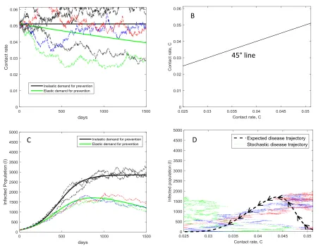
private demand for prevention is inelastic (contact rate is constant) and elastic (contact rate declines as diseases prevalence increases). The volatility in the infected population in Figures 2C and 3C reflect uncertainty in disease infectiveness and random events in births and mortality. The volatility in contact rates in Figures 2A and 3A reflects public health officials’ inability to
accurately predict human behavior. The expected and stochastic disease outcomes can be mapped into the 2-dimensional state space to illustrate the likelihood of observing specific combinations of 𝐼(𝑡) and 𝐶(𝑡). With private prevention lowering the contact rate over 6% per year, the
expected infected population 𝐸[𝐼] for each contact rate follows the dashed lines in Figures 2D and 3D. When gonorrhea is first detected in the population (𝐼0 = 100), the average number of
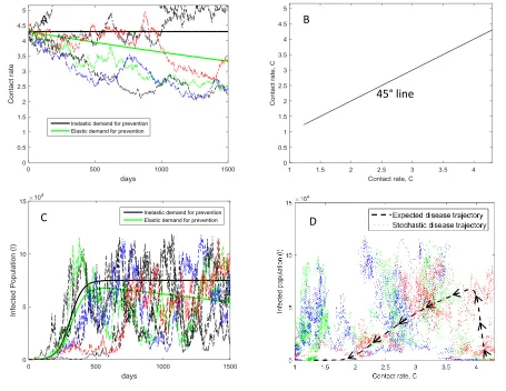
unprotected sexual encounters per year is 18 (𝐶0 = 0.05). As the infection spreads, the contact rate declines. Private prevention eventually causes the infected population to peak in a little over 2 years at 1700 infected individuals. When pneumococcus is first detected in the population (𝐼0 = 100), the average number of contacts per year is 1,569 (𝐶0 = 4.30). Private prevention eventually causes the expected infected population to peak in a little over 18 months at 67,405 infected individuals.
When private demand for prevention is inelastic, both diseases are expected to persist: 𝑅0𝐷 > 1. With private demand for prevention that is elastic, private prevention lowers the contact rate causing the economic-epidemiological system to eventually reach the disease-free
equilibrium. By hastening this decline in contact rates, the role of public health programs is to hasten the expected time to eradication within the population. However, the economic return from investing to hasten eradication depends on the likelihood of different disease and prevention outcomes. Points in Figures 2D and 3D show combinations of contact rate and prevalence
19
public prevention program will be less than expected when the infected population is lower than expected. An outbreak that is less severe than expected means fewer infections avoided due to the public health program and larger than expected program costs. Points above the dashed lines in Figures 2D and 3D indicate outcomes where the infected population is higher than expected while points below the dashed line indicate outcomes where the infected population is lower than expected. The points for pneumococcus are more dispersed along the y-axis indicating a
relatively greater amount of demographic stochasticity and uncertainty in disease infectiveness relative to uncertainty in contact behavior. Thus a large part of the risk associated with investing in a pneumococcus prevention program is associated with observing fewer avoided damages than expected.
Returns from the public prevention program will also be less than expected when the contact rate is lower than expected. When private prevention is more aggressive than expected, program costs are higher than expected and there is a greater likelihood that a negative shock to the contact rate may unexpectedly lead to eradication by crossing the bifurcation threshold. Points above and to the right of the dashed lines in Figures 2D and 3D indicate outcomes where the contact rate is higher than expected while points above and to the left of the dashed line indicate outcomes where the contact rate is lower than expected. Points below the dashed line may represent contact rates that are higher or lower than expected depending on whether
prevalence is rising or falling. The points for gonorrhea are more dispersed left to right indicating a relatively greater amount of uncertainty in contact behavior relative to environmental or
20
Optimal timing of gonorrhea and pneumococcus prevention programs
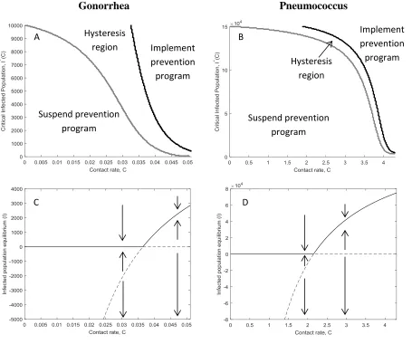
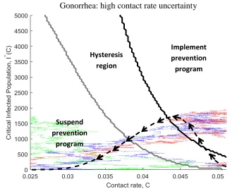
The optimal implementation and suspension curves for gonorrhea and pneumococcus prevention programs are presented in Figures 4A and 4B respectively. The optimality of public health intervention depends on both the incidence of disease 𝐼(𝑡) and the private provision of disease prevention 𝐶(𝑡). When the current state of the epidemic, defined by the pair (𝐼, 𝐶), is in the hysteresis region, no change should be made to the prevention program. A sufficiently large increase in the contact rate (rightward movement along the x-axis) or a sufficiently large increase in the infected population (upward movement along the y-axis) will justify a public prevention program. Once the program has been implemented, a sufficiently large decrease in the contact rate (leftward movement along the x-axis) or a sufficiently large decrease in the infected population (downward movement along the y-axis) will justify suspending the prevention program.
21
The implementation thresholds in Figure 4A and 4B account for the probability of each disease and private prevention outcome illustrated in Figures 2 and 3. They also account for the change in system stability that arises due to changes in the contact rate. There are two equilibria associated with the epidemiological model in equation (7). Figure 4C and 4D are bifurcation diagrams that show the stability of the endemic and disease-free equilibria implied from equation (7). When the contact rate is relatively high, the endemic equilibrium is stable and the disease-free equilibrium is unstable. The endemic equilibrium declines as private prevention lowers the contact rate. When the contact rate reaches 0.036 for gonorrhea and 2.1 for pneumococcus, the endemic equilibrium becomes unstable and the disease-free equilibrium becomes stable. As might be expected, program implementation is more likely when the endemic equilibrium is stable. Furthermore, a negative shock to the contact rate makes it more likely the disease is eradicated and less likely the public prevention program is implemented. However, a public prevention program may still be justified even if the disease is expected to die out due to the unpredictability of the epidemic.
Figure 5 overlays the expected and stochastic paths in Figures 2D and 3D over the
22
Geoffard and Philipson (1996) note that public health interventions may not be Pareto-optimal if they are undertaken too late. Our numerical results suggest that public health officials have a window of opportunity in which to intervene in the management of disease. Similar to Geoffard and Philipson, delaying gonorrhea and pneumococcus prevention programs too long raises the program’s costs which may eventually overwhelm potential benefits from preventing infection in a closed population. However, implementing programs too soon risks committing scarce funds to prevent diseases that are less damaging than anticipated either because
environmental or demographic variability significantly lower the prevalence of disease or private individuals adopt more preventative behavior than expected. For example, while gonorrhea and pneumococcus prevention programs are justified based on expected values of 𝐼(𝑡) and 𝐶(𝑡), some simulations never cross the implementation threshold. This incentive to “wait and see” reflects a reality for many federal agencies forced to sell or donate excess vaccines after dire predictions of an outbreak do not materialize.
Implications for program design and disease forecasting
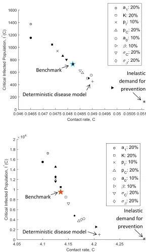
While we account for two different diseases, our numerical results are based on a single prevention program and a fixed degree of private prevention. Figure 6, investigates the sensitivity of the model to changes in private prevention behavior and characteristics of the public prevention program. The star in the center of the figure indicates the threshold for program implementation based on expected trajectories of the two stochastic variables and the parameter values in Table 1. Each symbol indicates how a change in a parameter shifts these implementation thresholds with filled symbols indicating an increase in the benchmark parameter value and open symbols
23
optimally implementing the program at a higher prevalence also means delaying until more private prevention has been undertaken.
As expected increases in program costs (𝐾, 𝑝𝐶), decreases in losses from infection (𝑝𝐼) or decreases in program effectiveness (𝑎1) make it optimal to delay program implementation until a larger number of people have become infected relative to the benchmark prevalence. These parameters shift the implementation and suspension curves in figure 5 but do not alter the expected path of the disease (dashed lines in figure 5), leading to predictable impacts on
responsiveness of public intervention. If 𝑎1 is selected to internalize the public good provided by individual prevention decisions, this result suggests that private prevention behavior that
generates a larger public good will also trigger a more expedient public health intervention.
The model also allows us to investigate how forecasts of 𝐼(𝑡) and 𝐶(𝑡) influence the responsiveness of public sector prevention programs (Figure 6). For our purposes, disease forecasts involve the mean (𝛽̃ and 𝑎0) and standard deviation (𝜎𝐶 and 𝜎𝛽) of the two stochastic variables. Changes in these forecast parameters shift the implementation and suspension curves in figure 5 and alter the expected path of the disease (dashed lines in figure 5). Compared to the benchmark, more optimistic forecasts of gonorrhea infectiveness (10% decrease in 𝛽̃) suggests the public prevention program should not be implemented in expectation. In contrast, more
optimistic forecasts of pneumococcus infectiveness delays program implementation in expectation.
24
implementation threshold – the public prevention program should not be implemented in
expectation. This result is consistent with the idea that public prevention programs and increasing disease prevalence compete to induce protective activity (Geoffard and Philipson, 1996). If forecasts assume the private demand for prevention is inelastic 𝑎0 = 0, the gonorrhea prevention program would be implemented when the infected population reaches 125 instead of 751 – nearly eleven months too soon. Likewise, the pneumococcus prevention program would be
implemented when the infected population reaches 170 instead of 9,500 – nearly seven months too soon. Failure to account for adaptive human behavior in epidemiological models may overestimate the expected return from public health interventions and encourage premature implementation of public health programs. This effect will be more pronounced the more elastic the actual private demand for prevention.
Changes in the forecast standard deviation or error are reflected by varying 𝜎𝐶 and 𝜎𝛽. Here we find that forecast error tends to delay program implementation due to the program’s option value. For the gonorrhea example, ignoring the error in private prevention forecasts suggests the program should be implemented when the infected population reaches 452 instead of 731. In the pneumococcus example, ignoring forecast error suggests the program should be implemented when the infected population reaches 1,025 instead of 9,500. In both cases, this is a difference of nearly 4 months in expectation. However, the impact of reducing forecast error depends on the disease context. For gonorrhea, reducing the forecast error associated with infectiveness has a minimal impact whereas reducing forecast error associated with private
25 Conclusions
Evaluating the cost-effectiveness of public health interventions requires forecasts of disease spread in order to predict the costs and benefits of prevention programs. However, inaccuracies in disease forecasts can lead to misleading conclusions about the persistence of disease, the tendency for private individuals to engage in prevention, and subsequently the returns provided from investing public funds in disease prevention programs. Considerable effort has been devoted to improve the accuracy of disease forecasts under the assumption public sector prevention programs will respond more quickly to disease outbreaks. We combine an optimal stopping model of public investment in disease prevention with stochastic models of disease and private prevention that provides a framework for quantifying the effect of improvements in disease forecasting on the timeliness of public responses to disease.
26
Bernanke’s “bad news principle” (Bernanke, 1983). This is in sharp contrast to previous findings about the implications of disease forecasts on private prevention decisions (Auld, 2003).
Second, improvements in disease forecasting may not make public health agencies more responsive to disease. If improvements in disease forecasting arise from a more complete account of individual incentives to engage in preventative behavior, public health interventions are likely to be less responsive to disease outbreaks. Elastic private demand for prevention implies lower expected returns from investing in prevention. In contrast, efforts to reduce the standard error of disease forecasts will tend to make the public sector more responsive to disease outbreaks. These second-moment improvements in disease forecasting tend to lower the option value associated with public health programs which lowers the burden of proof agency officials require to invest public funds in prevention.
27
epidemiological models. Finally the model focuses on preventative public health programs which reduce the contact rate. Many public health interventions involve immunization programs. Extending our model to account for this difference is left for future work.
Appendix
Demographic stochasticity following a Markov Chain process
We derive a system of stochastic differential equations that accounts for demographic stochasticity using a diffusion approximation to a continuous time Markov chain process. We consider the changes in both 𝑆 and 𝐼 populations and the probabilities associated with each
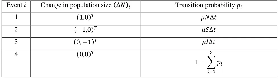
change in population size ("event") in a small time interval 𝛥𝑡. Individual-level events are discrete and can occur randomly. In a sufficiently small time interval, at most one event can occur. For example, individuals are born with probability (𝜇𝑁)𝛥𝑡 and the population size increases by one, i.e., 𝑆(𝑡 + 𝛥𝑡) → 𝑆(𝑡) + 1, or equivalently, 𝛥𝑁 = (𝛥𝑆, 𝛥𝐼) = (1,0)𝑇. The population changes and their probabilities obtained from the above assumptions are listed in Table A1.
We calculate the expectation and covariance for the changes in the two populations 𝑁𝑖 from the probabilities in Table A1. The expectation is 𝐸(𝛥𝑁) = ∑4𝑖=1𝑝𝑖(𝛥𝑁)𝑖, given by the 2 × 1 vector
𝜇𝛥𝑡 = 𝛥𝑡 (𝜇𝐼 − 𝛽𝐶𝑆 I 𝑁 𝛽𝐶𝑆 I
𝑁− 𝜇𝐼 ).
28
number of births of susceptible individuals is Poisson distributed with mean (𝜇𝑁)𝛥𝑡. Provided the transition probabilities (the rates at which events occur) are sufficiently large, we can approximate Poisson random variables by normal random variables. For example, we can write the recruitment rate as a normal random variable,
(𝛥𝑁)1 = (𝜇𝑁)𝛥𝑡 + √(𝜇𝑁)𝛥𝑡𝜂1,
where 𝜂1 is a unit normal random variable. Then the number of births is normally distributed with mean (𝜇𝑁)𝛥𝑡 and variance (𝜇𝑁)𝛥𝑡. Assuming the number of events in a time interval 𝛥𝑡 are Poisson distributed, we write down the following set of equations,
𝑆(𝑡 + 𝛥𝑡) = 𝑆(𝑡) + ∑ 𝑃𝑜𝑖𝑠𝑠𝑜𝑛 3
𝑗=1
(𝑝𝑗𝛥𝑡)(𝛥𝑆)𝑗
𝐼(𝑡 + 𝛥𝑡) = 𝐼(𝑡) + ∑ 𝑃𝑜𝑖𝑠𝑠𝑜𝑛 3
𝑗=1
(𝑝𝑗𝛥𝑡)(𝛥𝐼)𝑗
Using the normal distribution approximation to the Poisson distribution and denoting unit normal random variables by 𝜂𝑗, we obtain,
𝑆(𝑡 + 𝛥𝑡) = 𝑆(𝑡) + ∑ (𝑝𝑗𝛥𝑡 + √𝑝𝑗𝛥𝑡) (𝛥𝑆)𝑗 3
𝑗=1
𝜂𝑗
𝐼(𝑡 + 𝛥𝑡) = 𝐼(𝑡) + ∑ (𝑝𝑗𝛥𝑡 + √𝑝𝑗𝛥𝑡) (𝛥𝐼)𝑗 3
𝑗=1
𝜂𝑗
29
𝑆(𝑡 + 𝛥𝑡) = 𝑆(𝑡) + 𝜇1𝛥𝑡 + ∑ 𝐺1𝑗√𝛥𝑡𝜂𝑗 3
𝑗=1
𝐼(𝑡 + 𝛥𝑡) = 𝐼(𝑡) + 𝜇2𝛥𝑡 + ∑ 𝐺2𝑗√𝛥𝑡𝜂𝑗 3
𝑗=1
where 𝐺𝑖𝑗 = (𝛥𝑁𝑖)𝑗√𝑝𝑗⁄√𝛥𝑡. The resulting matrix
𝐺 = (√𝜇𝑁 −√𝜇𝑆 0
0 0 −√𝜇𝐼)
arising from the normal approximation to a Poisson distribution has the property that 𝐺𝐺𝑇 = 𝑉 (Allen et al., 2008). If 𝛥𝑡 → 0 and assuming the stochastic integral exists and is unique, then √𝛥𝑡𝜂𝑗 → 𝑑𝑧𝑗, where 𝑑𝑧𝑗 is a Wiener process. The equations converge to the system of stochastic differential equations,
𝑑𝑆 = (𝜇𝐼 − 𝛽𝐶𝑆 I
𝑁) 𝑑𝑡 + √𝜇𝑁𝑑𝑧1− √𝜇𝑆𝑑𝑧2
𝑑𝐼 = (𝛽𝐶𝑆 I
𝑁− 𝜇𝐼) 𝑑𝑡 − √𝜇𝐼𝑑𝑧3.
Table A1. Change in S and I populations and the probabilities associated with each change in the population size (event) in a small time interval ∆𝑡
Event i Change in population size (∆𝑁)𝑖 Transition probability 𝑝𝑖
1 (1,0)𝑇 𝜇𝑁∆𝑡
2 (−1,0)𝑇 𝜇𝑆∆𝑡
3 (0, −1)𝑇 𝜇𝐼∆𝑡
4 (0,0)𝑇
1 − ∑ 𝑝𝑖 3
30 Table 1. Epidemiological and economic parameters
Gonorrhea Pneumococcus
Description Value Source Value Source
Epidemiology
N Population 10,000 Gray et al. 2011 150,000 Lamb et al. 2011
𝐼0 Initial infected population 100 - 100 -
𝐶0 Initial contact rate 0.05 Yorke et al. 1978 4.30 Zhang et al. 2004
𝛽̃ Infectiveness mean 0.5 Thin 1970 0.01 -
𝜎𝛽 Infectiveness standard deviation 1e-6/C0 - 1e-6/C0 -
𝛾 Rate of recovery 0.018 Yorke et al. 1978 0.02 Lamb et al. 2011
𝜇 Mortality/birth rate 6.8e-5 Yorke et al. 1978 1.4e-3 Zhang et al. 2004
𝑅0𝐷 Deterministic reproductive number 1.40 Yorke et al. 1978 2.00 -
𝑅0𝑆 Stochastic reproductive number 0.35 - 1.97 -
Private response to disease
𝑎0 Private % reduction in contact rate 1.7e-4/day (6.2% annually)
𝜎𝐶 % volatility in contact rates 0.01
Public health program
𝑎1 Public % reduction in contact rate 3.4e-4/day (12.4% annually)
r Social planner discount rate 0.02 annually
K Sunk cost of prevention program 100
M Income per person 1
𝑝𝐼 Cost per infected individual 1
31
Figure 1. Private provision of disease prevention in the face of a growing epidemic
contacts C(t)
$
𝐶0
MB(C)
MC(C,0) MC(C,I)
Increasing prevalence of disease
Private supply of disease prevention Rising
32
Figure 2. Stability and expected outcomes of stochastic epidemiological model for
gonorrhea. (A) Expected (solid) and stochastic (dashed) paths for contacts rates when private demand for prevention is inelastic and elastic. (B) 45 degree line. (C) Expected (solid) and stochastic (dashed) paths for infected population when private demand for prevention is inelastic and elastic. (D) Disease outcomes in the two dimensional state space (𝐼, 𝐶).
45° line A
A
B
A
C
A
D
33
Figure 3. Stability and expected outcomes of stochastic epidemiological model for
pneumococcus. (A) Expected (solid) and stochastic (dashed) paths for contacts rates when private
demand for prevention is inelastic and elastic. (B) 45 degree line. (C) Expected (solid) and stochastic (dashed) paths for infected population when private demand for prevention is inelastic and elastic. (D) Disease outcomes in the two dimensional state space (𝐼, 𝐶).
45° line
A B
C
A
D
34
Gonorrhea Pneumococcus
Figure 4. Thresholds for disease persistence and public health intervention when demand for prevention is elastic. (A-B) Public prevention program implementation and suspension
thresholds. (C-D)Bifurcation diagram for the stability of the endemic and disease-free equilibria.
Implement prevention program Hysteresis
region
Suspend prevention program
Suspend prevention program
Implement prevention program Hysteresis
region A
A C
A
B A C
A
C C
A
D A C
35
Figure 5. Likelihood of implementing disease prevention program. Dashed lines represent the expected path of prevalence and contact rate. Dots show combinations of contact rate and
prevalence generated by three Monte Carlo simulations of the stochastic model.
Implement prevention program
Suspend prevention
program
Hysteresis region
Implement prevention program
Suspend prevention
program
Hysteresis region
Gonorrhea: high contact rate uncertainty
36
Figure 6. Impact of economic, epidemiology and uncertainty parameters on the expected
program implementation thresholds for (A) gonorrhea and (B) pneumococcus. Legend
indicates percent change in each parameter. Open symbols indicate a percent decrease in the benchmark parameter value while filled symbols indicate a percent increase in the benchmark parameter value
Benchmark
Inelastic demand for prevention Deterministic disease model
Inelastic demand for prevention Deterministic disease model
37 References
Aadland, D., Finnoff, D.C., Huang, K.X., 2013. Syphilis Cycles. The BE Journal of Economic Analysis & Policy 13, 297-348.
Allen, E.J., Allen, L.J., Arciniega, A., Greenwood, P.E., 2008. Construction of equivalent stochastic differential equation models. Stochastic Analysis and Applications 26, 274-297. Allen, L.J., 2003. An introduction to stochastic processes with applications to biology. Pearson Education Upper Saddle River, NJ.
Allen, L.J., Lahodny Jr, G.E., 2012. Extinction thresholds in deterministic and stochastic epidemic models. Journal of Biological Dynamics 6, 590-611.
Auld, M.C., 2003. Choices, beliefs, and infectious disease dynamics. Journal of Health Economics 22, 361-377.
Balikcioglu, M., Fackler, P.L., Pindyck, R.S., 2011. Solving optimal timing problems in environmental economics. Resource and Energy Economics 33, 761-768.
Bernanke, B.S., 1983. Irreversibility, Uncertainty, and Cyclical Investment. The Quarterly Journal of Economics 98, 85-106.
Brauer, F., Castillo-Chavez, C., 2011. Mathematical Models in Population Biology and Epidemiology. Springer.
Brekke, K., Øksendal, B., 1994. Optimal Switching in an Economic Activity under Uncertainty. SIAM Journal on Control and Optimization 32, 1021-1036.
Brito, D.L., Sheshinski, E., Intriligator, M.D., 1991. Externalities and compulsary vaccinations. Journal of Public Economics 45, 69-90.
Brooks, L.C., Farrow, D.C., Hyun, S., Tibshirani, R.J., Rosenfeld, R., 2014. Flexible Modeling of Epidemics with an Empirical Bayes Framework. PLOS Computational Biology 11.
Carman, K., Kooreman, P., 2014. Probability perceptions and preventive health care. J Risk Uncertain 49, 43-71.
Chen, F., Toxvaerd, F., 2014. The economics of vaccination. Journal of Theoretical Biology 363, 105-117.
Chen, F.H., 2009. Modeling the effect of information quality on risk behavior change and the transmission of infectious diseases. Mathematical Biosciences 217, 125-133.
Chow, Y.S., Robbins, H., Siegmund, D., 1971. Great Expectations: The Theory of Optimal Stopping. Houghton Mifflin Boston.
38
Evans, W.N., Viscusi, W.K., 1991. Estimation of state-dependent utility functions using survey data. The Review of Economics and Statistics, 94-104.
Fenichel, E.P., Castillo-Chavez, C., Ceddia, M.G., Chowell, G., Parra, P.A.G., Hickling, G.J., Holloway, G., Horan, R., Morin, B., Perrings, C., Springborn, M., Velazquez, L., Villalobos, C., 2011. Adaptive human behavior in epidemiological models. Proceedings of the National
Academy of Sciences 108, 6306-6311.
Fenichel, E.P., Wang, X., 2013. The mechanism and phenomena of adaptive human behavior during an epidemic and the role of information, in: Manfredi, P., D'Onofrio, A. (Eds.), Modeling the Interplay Between Human Behavior and the Spread of Infectious Diseases, Vol. Volume|, Edition ed|. Publisher|, City|, p.^pp. Pages|.
Francis, P.J., 1997. Dynamic epidemiology and the market for vaccinations. Journal of Public Economics 63, 383-406.
Geoffard, P.-Y., Philipson, T., 1996. Rational epidemics and their public control. International Economic Review, 603-624.
Geoffard, P.-Y., Philipson, T., 1997. Disease eradication: private versus public vaccination. The American Economic Review, 222-230.
Gersovitz, M., Hammer, J.S., 2004. The Economical Control of Infectious Diseases. The Economic Journal 114, 1-27.
Gersovitz, M., Hammer, J.S., 2005. Tax/subsidy policies toward vector-borne infectious diseases. Journal of Public Economics 89, 647-674.
Gray, A., Greenhalgh, D., Hu, L., Mao, X., Pan, J., 2011. A stochastic differential equation SIS epidemic model. SIAM Journal on Applied Mathematics 71, 876-902.
Gualtieri, A.F., Hecht, J.P., 2011. Dynamics and Control of Infectious Diseases in Stochastic Metapopulation Models. Journal of Life Sciences 5, 503-508.
Hethcote, H.W., Yorke, J.A., 1984. Gonorrhea Transmission Dynamics and Control. Springer-Verlag, Berlin.
Huang, S.S., Johnson, K.M., Ray, G.T., Wroe, P., Lieu, T.A., Moore, M.R., Zell, E.R., Linder, J.A., Grijalva, C.G., Metlay, J.P., 2011. Healthcare utilization and cost of pneumococcal disease in the United States. Vaccine 29, 3398-3412.
Jacquez, J.A., O'Neill, P., 1991. Reproduction numbers and thresholds in stochastic epidemic models I. Homogeneous populations. Mathematical Biosciences 107, 161-186.
Judd, K., 1998. Numerical Methods in Economics. MIT Press.
39
Kremer, M., 1996. Integrating Behavioral Choice into Epidemiological Models of AIDS. The Quarterly Journal of Economics 111, 549-573.
Kureishi, W., 2009. Partial vaccination programs and the eradication of infectious diseases. Economics Bulletin 29, 2758-2769.
Lamb, K.E., Greenhalgh, D., Robertson, C., 2011. A simple mathematical model for genetic effects in pneumococcal carriage and transmission. Journal of Computational and Applied Mathematics 235, 1812-1818.
Laporte, R.E., 1993. How to improve monitoring and forecasting of disease patterns. BMJ 307, 1573-1574.
LaRiviere, J., Wolff, H., 2015. The Power of the Little Blue Pill: Innovations and Implications of Lifestyle Drugs in an Aging Population. Economic Inquiry 53, 540-556.
Marten, A.L., Moore, C.C., 2011. An options based bioeconomic model for biological and chemical control of invasive species. Ecological Economics 70, 2050-2061.
McChlery, S.M., Scott, K.J., Clarke, S.C., 2005. Clonal analysis of invasive pneumococcal isolates in Scotland and coverage of serotypes by the licensed conjugate polysaccharide
pneumococcal vaccine: possible implications for UK vaccine policy. Eur J Clin Microbiol Infect Dis 24, 262-267.
Miranda, M., Fackler, P.L., 2002. Applied Computational Economics and Finance. The MIT Press.
Nævdal, E., 2012. Fighting Transient Epidemics—Optimal Vaccination Schedules Before And After An Outbreak. Health Economics 21, 1456-1476.
Nsoesie, E., Mararthe, M., Brownstein, J., 2013. Forecasting peaks of seasonal influenza epidemics. PLoS Currents 5.
O’Regan, S.M., Drake, J.M., 2013. Theory of early warning signals of disease emergenceand leading indicators of elimination. Theoretical Ecology 6, 333-357.
Philipson, T., Posner, R., 1993. Private choices and public health: The AIDS epidemic in an economic perspective. Harvard University Press, Cambridge, MA.
Pindyck, R.S., 2007. Uncertainty in Environmental Economics. Rev Environ Econ Policy 1, 45-65.
Qi, H., Liao, L., 1999. A Smoothing Newton Method for Extended Vertical Linear
40
Shaman, J., Karspeck, A., 2012. Forecasting seasonal outbreaks of influenza. Proceedings of the National Academy of Sciences 109, 20425-20430.
Shiller, R.J., Pound, J., 1989. Survey evidence on diffusion of interest and information among investors. Journal of Economic Behavior & Organization 12, 47-66.
Soebiyanto, R.P., Adimi, F., Kiang, R.K., 2010. Modeling and predicting seasonal influenza transmission in warm regions using climatological parameters. PloS one 5, e9450.
Stoneman, P., 1983. The economic analysis of technological change. Oxford University Press. Thin, R., 1970. Immunofluorescent method for diagnosis of gonorrhoea in women. British Journal of Venereal Diseases 46, 27.
Van den Driessche, P., Watmough, J., 2000. A simple SIS epidemic model with a backward bifurcation. Journal of Mathematical Biology 40, 525-540.
Wayne, A., 2014. Obamacare Website Costs Exceed $2 Billion, Study Finds, Bloomberg Business.
Wickwire, K., 1977. Mathematical models for the control of pests and infectious diseases: a survey. Theoretical Population Biology 11, 182-238.
Xu, X., 1999. Technological improvements in vaccine efficacy and individual incentive to vaccinate. Economics Letters 65, 359-364.
Yorke, J.A., Hethcote, H.W., Nold, A., 1978. Dynamics and control of the transmission of gonorrhea. Sexually Transmitted Diseases 5, 51-56.