Environmental Resources Research Vol. 5, No. 2, 2017
GUASNR
Compactness for Regionalization and its Application in
Land-Use Planning
M. Saeed sabaee1*, A. Salmanmahiny2, S.M. Shahraeini3, S.H. Mirkarimi4, N. Dabiri5
1Ph.D candidate in Environmental Science, Gorgan University of Agricultural Sciences and Natural Resources, Gorgan, Iran 2
Dept. of Environmental Science, Gorgan University of Agricultural Sciences and Natural Resources, Gorgan, Iran. 3
Dept. of Electrical Engineering, Faculty of Engineering, Golestan University, Gorgan, Iran. 4
Dept. of Environmental Science, Gorgan University of Agricultural Sciences and Natural Resources, Gorgan, Iran. 5Dept. of Industrial Engineering, Faculty of Engineering, Golestan University, Gorgan, Iran.
Received: August 2016 ; Accepted: December 2016
Abstract
One of the most important and appealing subjects discussed and applied in many geographical studies is compactness. This is a geometrical notion and has applications far beyond the scope of its definition. Besides the importance of measuring compactness in a single object, its study is significant in real-world applications, where the integration of items or objects in conjunction with each other is considered. Regionalization is the term commonly used for this integrative perspective. Although there are several methods to quantify compactness, this study tries to illustrate the simple way for its calculation. Hence, this study is devised to apply with some modifications one of the methods that has been suggested for calculating single object compactness in regionalization domain. We attempt to propose a clear definition and to evaluate the computer implementation of the compactness in a land-use planning study. The ant colony algorithm as a heuristic approach was applied to measure compactness in an innovative manner and to incorporate this concept into a land-use planning case. Results show that this method can be useful in achieving compactness in land-use planning.
Keywords: Compactness, Regionalization, Land-use planning, Ant colony
Introduction
Compactness is a geometrical and topological notion and under this domain its definition is rather difficult. However, as a shape index it refers to a numerical quantity to describe the degree or intensity of compactness of a shape (Gillman, 2002). Compactness has been an appealing notion and research question because of longstanding use and significant number of its applications.
Compactness measurement has many applications including political districts designing (Harris, 1964; Kaiser, 1966; Hofeller and Grofeman, 1990), selecting the spatial regions that share special properties (Wentz, 1997), defining the hydrological attributes of drainage basins (Bardossy and Schmidt, 2002), city designing (Cao and Huang, 2010) and measuring the connectivity in sustainable and green city planning (C. Y., 2004; Crewe and Forsyth, 2011). In natural resources domain, compactness as a shape index could be used for many reasons, such as forecasting future patterns, selecting suitable habitats, designing natural reserves, understanding geographical phenomena, defining the situation of landscape or even land-use planning.
Land-use planning, as an
interdisciplinary study, seeks to establish equilibrium among economic, social and political development along with environmental conservation. In fact, this practice is a branch of management and needs criteria for analyzing. Regardless of many explicit economic criteria, there are implicit conservation criteria extracted and inspired from the environment, of which compactness is one of the most important items.
Human activities decrease total area of natural ecosystems. This decreasing trend can cause separation and fragmentation of the natural form of ecosystems and also it can divide them into smaller pieces. Hence, fragmentation may happen in conjunction with ecosystem downsizing (Rutledge, 2003). The fragmentation process has a broad range of effects on ecosystems such as resource availability, distribution, flow of natural and artificial resources
(organisms, propagules, nutrients, machines, infrastructures, services) and finally it can influence human life (Rutledge, 2003). In general, loss and fragmentation of an ecosystem is a vigorous challenge for land management and such a process may affect fauna, flora and humans as effective components of ecosystems.
perimeter and area or even comparing it with the same relationship in a reference shape (circle), has been a topic of research (as a classical approach) in compactness calculation. Different methods have been proposed to accomplish this target. Simple area to perimeter ratio has been suggested by Ritter in 1822(Frolov, 1975) that has gradually been modified to a dimensionless model (Eq. 1). Because the simple perimeter/area ratio varies with changes in shape size, the square root of the area or squaring the perimeter value has been proposed for solving this problem and making dimensionless ratio (Miller, 1953). This modified ratio has been simplified to a model with more practical range (Eq. 2). By adding π, the range of Miller's ratio is changed between 0 to 1(Osserman, 1978): Eq.(1) =
Eq.(2) =
In all these methods, shape is a unique object. In other words, in this method, shape is a single polygon with a discrete boundary. Such viewpoint is supported by vector data model. Compared with this model, there is a raster data model that is more consistent with the quality of converting information into a computer-friendly form. In this model, any shape is
divided into a number of regular cells named pixels. Although in vector data model, the closer to the circle, the more compact is an object; in raster data model, the closer to the square, the more compact it is. Here, we see a reference to the fact that among all rectangles with equal area, square has the smallest perimeter that is equal to four times the square root of its area (Hoshino, 2015). Equation (3) for compactness calculation has been modified on the basis of such logic (Frohn, 1998; Farina, 1998; McGarigal and Marks, 1993; Bogaert and Impens, 1998):
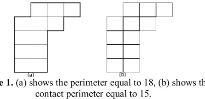
Eq. (3) = √ In raster domain, Bribiesca (1997) proposed a method for calculating compactness of a single shape based on the score range procedure of data standardization. The initial assumption of this method is that a single isolated shape is composed of cells with equal length of sides considered one. Also, there are two basic definitions in this method, perimeter and contact perimeter. Perimeter is the sum of the sides of pixels that are not shared by other pixels. This means outer sides of the closed shape. Contact perimeter is the sum of the sides of pixels that are shared between pixels (Figure 1).
Figure 1. (a) shows the perimeter equal to 18, (b) shows the contact perimeter equal to 15.
Bribiesca (1997) found a relation between perimeter and contact perimeter. For this relation, if the length of each side is one, equation (4) can be used as the following: Eq.(4) = 4 − 2
Where P is the perimeter, CP is the contact perimeter and n is the number of pixels composing a shape. Then, in order to connect this information to a benefit criterion for showing intensity of shape compactness, Bribiesca applied the score range procedure. For this, the standardized
score is calculated by dividing the difference between a calculated raw score and the minimum score to the difference between the maximum and the minimum scores (Malczewski, 1999). Equation (5) shows the standardized measure of compactness (CSC) proposed by Bribiesca.
Eq.(5) =
In all issues mentioned above, shape is still illustrated as a single and isolated object. In comparison with this view, there is another real-world view where there are many cases in which a shape is defined in conjunction with the other shapes. This subject is named regionalization (Li et al., 2013). Land-use planning or land-use allocation is a case of regionalization. In this process, proportion and location of different land uses as the best possible optimal configuration, are determined within a special area (Liu et al., 2012). With this simple definition, this issue is a case of optimization. Many different criteria are used in this process, some of which conflict to each other. Among the large collection of the criteria, compactness is one of the most important. Many researchers proposed some methods for calculating compactness in regionalization problems. Although these methods are different in details, many of them are proposed on the basis of classical approach of compactness calculation mentioned before (Minor & Jacob, 1994; Wright et al., 1983; Gilbert et al., 1985; Liu et al., 2012). This study tries to address calculating and optimizing compactness in land-use planning as regionalization problem. to
meet the aim of the study, Bribiesca's model used for calculating compactness in single shape was applied and modified for calculating compactness in a space containing some fragmented shapes. these modifications stated as some equations and applied in a heuristic algorithm in order to be tested.
Materials and Method
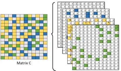
To explain how to introduce compactness to a land-use configuration study, we assume the study area as a matrix and its land uses as different kinds of colors of the matrix. The side length of every pixel in this matrix is one. The number of pixels of every colorful collection is equal to the number of regular pieces of land located by every land use. Hence, sum of the pixels in all colorful collections is equal to total pixels of matrix and also total area of the considered land with respect to its scale. This randomly distributed colors represents dispersed elements of shapes with different colors. Simply, it is possible to imagine this matrix as transparent layers overlaid on each other. Each transparent layer refers to each dispersed shape or each colorful collection of pixels. We can distinguish hollow pixels with 0 and colored pixels with 1 in each layer (Figure 2).
Figure 2. Matrix C with four kinds of colors is like four transparent layers precisely overlaid on each other
In this situation, the purpose is making an optimal configuration in the matrix such that the same colored pixels are located adjacent to each other and final closed shapes are produced.
It is necessary to say that a number of algorithms have been proposed to find the optimal configuration (Williams and
maximizing desired factors or minimizing undesired ones. Compactness is one of the commonly used desired factors. Creation of an initial random configuration of land uses is the first step in many of these specific algorithms. Then, this raw initial configuration is gradually improved based on the objective function value of the algorithm.
With the imagination that every kind of land uses is assumed as special color, the first iteration is started with a random configuration of colors in a matrix which will be modified step by step with the improvement of compactness value (function value) during the next iterations. However, there are four parameters that must be determined for compactness calculation:
1. Current compactness in each iteration 2. Minimum compactness
3. Maximum compactness
4. Normalized value of current compactness in each iteration
These parameters must be calculated for every colorful collection of pixels in every iteration and finally compactness will be calculated by summing normalized value of current compactness for all collections. Odd or even number of pixels in the matrix affects compactness calculation, however, these two steps should be undertaken as below:
Step 1: Current compactness or contact perimeter ( ) of every dispersed shape (every colorful collection of pixels) within the matrix is calculated using equation (6).
Eq.(6)
=
4 −2
In this equation, ( ) refers to each colored collection (kind of land uses). Therefore ( ), ( ) and ( ) are respectively the perimeter, the contact perimeter (current compactness) and the number of pixels in every colorful collection.
Step 2: There are three possibilities for minimum compactness calculation in a matrix with odd pixels as follows:
2.A: if the number of pixels refers to a collection ( ) equals to an absolute value of the total number of matrix pixels divided by two plus four, the minimum compactness of every colored collection ( ) is calculated by equation (7):
≤ ×
2 + 4 ≤ Eq.(7) ℎ = 4 ( ) and ( ) refers to the rows and columns of matrix of study area. To facilitate describing the following equations, ( × + 4) at the first line of equation (7) is substituted with ( ).
2.B: if the number of pixels containing a collection ( ) is ranged between the two following values, the minimum compactness ( ) is characterized by equation (8):
< ≤ + 2
2 + 2
− 4 < ≤ +
Eq.(8) ℎ = 4 − 2
Like previous equation, ( 2 + −
4 at the first line of equation (8) is replaced with ( ) to ease describing the third equation.
2.C: if the number of pixels composing a collection is higher than the following value, the minimum compactness is calculated as follows (equation 9):
> +
ℎ calculate: = − ( + )
Eq.(9) = 4 − (2 + 4 ) In fact, when the number of pixels
Figure 3. Four neutral corners in matrix with odd pixels
For the second possibility, the number of extra pixels assigned to the collection is equal to the number of hollow pixels in the boundary of matrix without accounting for neutral corners (B). In this situation, by
allocating every pixel to the collection, for every three unshared sides eliminated, one unshared side is added (Figure 4). This difference is the logic behind equation (8).
Figure 4. Changes in the boundary of matrix when 1 pixel is added
The last possibility is the situation in which the number of extra pixels assigned to the collection is more than B. In this situation, for every new pixel assigned to the collection, four unshared sides are converted to shared sides and no unshared side is generated.
Similar to the matrix with odd pixels, there are nearly the same three possibilities in calculating the minimum compactness of
the matrix with even pixels. However, in the second possibility of this form of matrix, instead of four corners, there are two corners that are neutral towards allocating pixels to collections (Figure 5). Table (1) shows changes in equations 7, 8, 9 for a matrix with even pixels. These changes are in conjunction with a little change in A and B.
Table 1. Changes in equations 7,8,9 for a matrix with even pixels
≤ ×
2 + 4
(7) ℎ = 4
≤ ×
2 + 2
(7∗∗) ℎ = 4
< ≤ + ((2
2 + 2 ) − 4) (8) ℎ = 4 − 2
< ≤ + ((2
2 + 2 ) − 2) (8∗∗) ℎ = 4 − 2 > +
(9) ℎ : = − ( + )
= 4 − (2 + 4 )
> +
(9∗∗) ℎ : = − ( + )
= 4 − (2 + 4 )
** means equations changed for matrix with even pixels
Step 3: since the area of every pixel equals one, we can say that the sum of pixels of a collection denotes its area. Thus, the maximum compactness of a collection of pixels within matrix that points to square shape can be characterized by equation 10. Eq.(10) = 4 Where (Pxk) is the number of pixels
referring to a collection.
Step 4: In this step, parameters calculated in the three previous steps are applied to equation (11). The result is a standardized value of compactness ( ).
Eq.(11) =∑ ( −
− )
=1
As it was stated before, this standardized value must be calculated for every collection of matrix pixels and in every iteration. The final compactness value in every iteration is the sum of standardized
compactness calculated for all collections of course, depending on the algorithm used, the implementation strategy is slightly different. Figure 6 summarizes all mentioned steps that must be followed for calculating standardized value of compactness.
Computer implementation, Results & Discussion
To test the measure of compactness, a matrix with 53 rows and 77 columns was selected. We decided to assign a fixed number of pixels from four collections into the matrix. In fact, the purpose was to locate pixels of every collection as much close as possible to each other. Table 2 shows the required number of pixels in every collection.
Table 2. The number of pixels assigned to every collection
Collection Number of pixels
A 700
B 650
C 2170
D 561
Ant Colony Optimization as a heuristic algorithm was chosen for this purpose. It is implemented using MATLAB Version 7.12.0. Although explaining the algorithm is beyond the scope of this paper, general stages can be stated as follows:
1- Entering initial data (the required pixels of every collection)
Figure 6. Steps for calculation standardized value of compactness
3-Initializing: evoking the objective function, defining special parameters of the algorithm, setting the number of iterations, creating enough empty space for saving the value of function in every iteration and defining the stopping criteria for the algorithm.
4-Writing the main loop: in this step, on the basis of specific structure of probabilities, new configuration for each iteration is determined. Then, the value of objective function is calculated, and is compared with values of the previous iterations and the best one is selected. This process continues until the stopping criteria causes it to finish. Minimum Compactness
1 2 3 3 2 1
No....is Even is Odd....Yes
if the whole number of matrix pixels is
Calculate the number of the collection pixels ( ) and the whole number of matrix pixels
×
Minimum Compactness
Current Compactness Maximum Compactness
Fig (7-a) Fig (7-b)
Fig (7-c)
Figure 7. (a, b, c) configuration of colored pixels in iteration 1 (5-a), iteration 5 (5-b) and iteration 10 (5-c)
Figures (7-a), (7-b) and (7-c) respectively show distribution and configuration of colored pixels in iteration 1 (t=0), iteration 5 (t=4) and iteration 10 (t=9). As it is clear in figure (7-c), the improvement of compactness is apparent
after 10 iterations. Figure (8) represents a positive trend of compactness value changes during iterations. The x axis indicates iteration and the y axis shows the value of compactness.
Figure 8. Improvement of Compactness value with iterations
In attempting to find the best result, compactness in a land-use planning study was considered. For this purpose, an area about 397km2 of Gorgan Township located in Golestan province in the northern part of Iran was chosen. This area is located at latitudes between N 36˚ 43ʹ 7ʺ and 36˚ 56ʹ 45ʺ and longitudes between E 54˚ 24ʹ 47ʺ and 54˚ 37ʹ 59ʺ. The whole case study area is a
matrix with 132 rows and 127 columns with a spatial resolution of 150 m. It includes four general land uses: agriculture, forest, range and residential areas (or developed land). table (3) shows current area of every land use. The study area has been covered with some small and dispersed land uses including roads, rivers and water body. Since current configuration
1.5 1.75 2 2.25 2.5 2.75 3
0 1 2 3 4 5 6 7 8 9 10 11
C
o
m
p
ac
tn
e
ss
of land uses has been generated without paying attention to suitability of the land, proposing the best optimal configuration of
land uses based on land suitability and compactness criteria were further studies.
Table 3. The area assigned to land uses in the study area
Land use Area (Km2)
Agriculture 169.96
Forest 181.27
Development 28.39
Range 0.28
Main Road 4.92
Secondary Road 7.67
Water body 0.90
River 3.22
Water bodies, rivers, roads and current developed areas were excluded from the study area because they are usually not transformable to other uses. The remaining area was about 350.50 km2. Regarding land suitability of the study area, we attempted to optimize four general land uses based on a set of predetermined proportions. The defined areas of all land uses are shown in Table (4). The last column of this tables shows equivalent area of land uses in cell unit. optimality is determined on the basis of suitability degree and compactness value of land uses. The suitability map for each land use type was generated using many
ecological attributes such as "elevation, slope, geomorphology, geology, soil texture and fertility, EC and soil hydrological groups, temperature, evaporation, precipitation, density of green cover of land, depth of ground water, distance to river, town, roads, water bodies and some other attributes" (Salmanmahiny et al., unpublished).
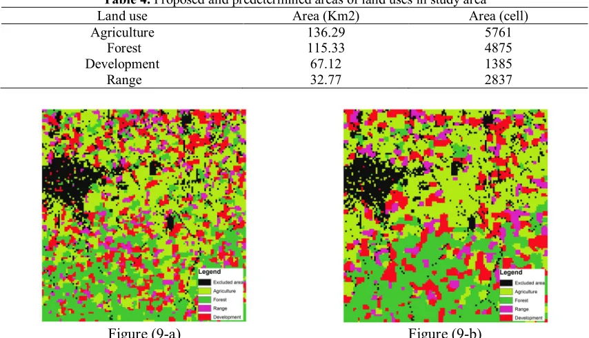
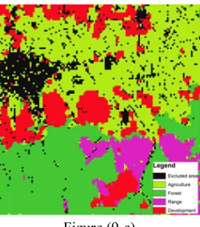
The ant colony algorithm was used for optimization. Figure (9-a), (9-b) and (9-c) show changes in configuration of land uses according to suitability and compactness of land uses.
Table 4. Proposed and predetermined areas of land uses in study area
Land use Area (Km2) Area (cell)
Agriculture 136.29 5761
Forest 115.33 4875
Development 67.12 1385
Range 32.77 2837
Figure (9-c)
Figure 9. (a, b, c) configuration of land uses in iteration 10 (9-a), iteration 50 (9-b) and iteration 100 (9-c)
Table 5 shows the compactness degree of figures (9-a, b and c) respectively. Since the cost of land use is one of the initial factors in land-use planning, in this example besides paying attention to compactness,
allocation cost of land to special use was considered. Therefore final configuration shows result as real and practical as possible.
Table 5. Compactness degree for every land uses in iterations 10, 50 and 100
Type of land use Compactness degree in iterations
Iteration10 Iteration50 Iteration100
Agriculture 0.7269 0.7997 0.8165
Forest 0.7633 0.8644 0.8915
Range 0.5416 0.7097 0.7405
Development 0.6376 0.7549 0.7995
Results of table (5) is quite revealing the promotion of the intensity of compactness from iteration 10 to 100. Also results from table (5) can be compared with the trend of compactness value in test 1 in figure (8) (matrix with 53 rows and 77 columns). Both of these two tests indicate that the proposed equations were successful in optimizing compactness value in space containing more than one shape. applying the relationship between perimeter and area in calculating compactness has been reported in previous research. For example, Minor and Jacob (1994) applied such a classical approach to attain compactness in land allocation for waste landfill sitting, Wright et al., (1983) and Gilbert et al., (1985) separately considered use of compactness criterion besides some other criteria in small land acquisition problem in study era respectively with (25 × 25) pixels and 900 pixels. All the researchers utilized linear programming to define compactness equations. Although the results of current
study show the improvement of compactness value in larger study area, this may be affected by the inherent limitation of linear programming used in previous research. Liu et al., 2012 also use the standardized criterion for addressing compactness in land-use optimization problem, but this study attempts to set out considering compactness in details with some modifications in terms of some equations.
Conclusion
groups' elements in the calculation space. This is the same subject used in the regionalization issue. It seems that simplicity is the power of this measure which makes it more comprehensible and possible to use in programming and writing algorithms. Although in many cases of regionalization there are many other criteria used in analyzing, compactness and contiguity are two of the most important criteria used in configuration of features such as land uses especially from the managers' point of view. Therefore, attention to this criterion is very important. Optimization and conflict resolution methods such as Multi-Objective Land
Allocation (MOLA) offered by Eastman et al. in TerrSet version of IDRISI in 2014 have tried to include landscape metrics in the procedure. However, these applications suffer from calculation time or compromises in terms of suitability or landscape metrics and often can only handle very simple tasks. We have shown here that using a simple approach to calculate compactness and incorporating it into the process of land use conflict resolution can overcome part of this problem. However, more work needs to be implemented to further the approach used here and make it suggestable as a user friendly method of land use planning.
References
Aerts, J.C.J.H., Eisinger, E., Heuvelink, G.B.M., and Stewart, T.J. 2003. Using Linear Integer Programming for Multi-Site Land- Use Allocation. Geographical Analysis, 35(2), 148-169.
Bardossy, A., and Schmidt, F. 2002. GIS Approach to Scale Issues of Perimeter-based Shape Indices for Drainage Basins. Hydrological Sciences Journal, 47(6), 931-942.
Bogaert, J., and Impens, I. 1998. An improvement on area-perimeter ratios for interior-edge evaluation of habitats. In: F. Muge, R.C. Pinto, M. Piedade (eds.) Proceedings of the 10th Portuguese Conference on Pattern Recognition, Lisbon, Portugal. 55-61.
Bribiesca, E. 1997. Measuring 2-D Shape Compactness Using the Contact Perimeter. Computers and Mathematics with Applications, 33(11), 1-9.
C.Y J. 2004. Green-space Preservation and Allocation for Sustainable Greening of Compact Cities. Cities Journal, 21(4), 311-320.
Cao, K., and Huang, B. 2010. Comparison of Spatial Compactness Evaluation Methods for Simple Genetic Algorithm based Land Use Planning Optimization Problem. Proceedings of the Joint International Conference on Theory, Data Handling and Modelling in GeoSpatial Information Science, 38(2), 26-28.
Crewe, K., and Forsyth A. 2011. Compactness and connection in Environmental Design: Insights from Ecoburbs and Ecocities for Design with nature. Environment and Planning B: Planning and Design, 38, 267-288.
Didham, R.K. 1998. ''Altered Leaf-litter Decomposition Rates in Tropical Forest Fragments''. Oecologia. 116(3), 397-406.
Farina, A. 1998. ''Principles and Methods in Landscape Ecology''. Chapman & Hall, University Press, Cambridge. 412 P
Frohn R.C. 1998. Remote Sensing for Landscape Ecology; New Metric Indicators for Monitoring, Modelling, and Assessment of Ecosystems. Lewis Publishers, CRC Press LLC, Boca Raton, 112 P. Frolov, Y.S. 1975. Measuring of Shape of Geographical Phenomena: A History of Issue. Soviet
Geography: Review and Translation, 16(10), 676-687.
Gilbert, K.C., Holmes, D.D., and Rosenthal, R.E. 1985. A Multiobjective Discrete Optimization Model for Land Use Allocation. Management Science, 31, 1509-1522
Gillman, R. 2002. Geometry and gerrymandering. Math Horizons, 10(1), 10-13.
Guiliano, G., and Narayan, D. 2003. Another Look at Travel Patterns and Urban Form: the US and Great Britain. Urban Studies, 40(11), 2295-2312.
Harris, C.C. 1964. A Scientific methods of Distribution. Behavioral Science, 9, 219-225.
Hofeller, T., and Grofman, B. 1990. Comparing the Compactness of California Congressional Districts under Three Different Plans: 1980, 1982, and 1984. In Toward fair and Effective Representation ed. B. Grofeman, New York: Agathon.
Kaiser, H. F. 1966. An Objective Method for Establishing Legislative Districts. Midwest Journal of Political Science, 10, 200-213.
Li, W., Goodchild M.F., and Church, R.L. 2013. An Efficient of Compactness for Two Dimensional Shapes and its Application in Regionalization Problems. International Journal of Geographical Information Science, 27(6), 1227-1250.
Liu. X., Li, X., Shi, X., Huang, K., and Liu, Y. 2012. A Multi-type Ant Colony Optimization (MACO) Method for Optimal Land use Allocation in Large Areas. International Journal of Geographical Information Science, 26(7), 1325-1343.
Malczewski, J. 1999. GIS and Multicriteria Decision Analysis. Wiley. 392 P.
McGarigal K., and Marks B. 1993. Fragstats: Spatial Pattern Analysis Program for Quantifying Landscape Structure. Oregon State University, Forest Science Department. 122 P.
Miller, V.C. 1953. A Quantitative Geomorphic Study of the Drainage Basin Characteristics in the Clinch Mountain Area, Virginia and Tennessee. New York: Columbia University Department of Geology Technical Report. 3.
Minor, S.D., and Jacobs, T.L. 1994. Optimal Land Allocation for Slid and Hazardous Waste Landfill Sitting. Journal of Environmental Engineering, 120, 1095-1108.
Osserman, R. 1978. Isoperimetric Inequality. Bulletin of American Mathematical Society, 84(6), 1182-1238.
Patton, D. R. 1975. A Diversity Index for Quantifying Habitat Edge. Wildlife Society Bulletin, 3 (4), 171-173.
Rutledge, D. 2003. Landscape Indices as measures of The Effects of Fragmentation: Can Pattern Reflect Process? Published by Department of Conservation, Wellington, New Zealand. 26 P.
Saunders, D.A., Hobbs, R.J., and Margules, C.R. 1991. Biological Consequences of Ecosystem Fragmentation: A Review. Conservation Biology, 5(1), 18-32.
Stewart, T.J., Janssen, R., and Herwijnen, M.V. 2004. A Genetic Algorithm Approach to Multi objective Land use Planning. Computer and Operation Research, 31(14), 2293-2313.
Walmsley, A.J., Walker, D.H., Mallawaarachchi, T., and Lewis, A. 1999. Integration of Spatial Land use Allocation and Economic Optimization Models for Decision Support. In. MODSIM 99: International Congress on Modelling and Simulation: Modelling and Simulation Society of Australia.
Wentz, E.A. 1997. Shape analysis in GIS. In Annual Convention & Exposition Technical Papers, AutoCarto, 13(5), 204-213.
Williams, J.C. and ReVelle, C.S. 1998. Reserve Assembla e of Critical Areas: A Zero-One Programming Approach. European Journal of Operational Research, 104(3), 497-509.
Williams, K.1999. Urban Intensification Policies in England: Problems and Contradictions. Land Use Policy, 16(3), 167-178.