www.wind-energ-sci.net/2/77/2017/ doi:10.5194/wes-2-77-2017
© Author(s) 2017. CC Attribution 3.0 License.
An error reduction algorithm to improve lidar turbulence
estimates for wind energy
Jennifer F. Newman1and Andrew Clifton2
1National Wind Technology Center, National Renewable Energy Laboratory, Golden, CO 80401, USA 2Power Systems Engineering Center, National Renewable Energy Laboratory, Golden, CO 80401, USA
Correspondence to:Jennifer F. Newman ([email protected])
Received: 27 June 2016 – Discussion started: 8 July 2016
Revised: 22 December 2016 – Accepted: 16 January 2017 – Published: 10 February 2017
Abstract. Remote-sensing devices such as lidars are currently being investigated as alternatives to cup anemometers on meteorological towers for the measurement of wind speed and direction. Although lidars can measure mean wind speeds at heights spanning an entire turbine rotor disk and can be easily moved from one location to another, they measure different values of turbulence than an instrument on a tower. Current methods for improving lidar turbulence estimates include the use of analytical turbulence models and expensive scan-ning lidars. While these methods provide accurate results in a research setting, they cannot be easily applied to smaller, vertically profiling lidars in locations where high-resolution sonic anemometer data are not available. Thus, there is clearly a need for a turbulence error reduction model that is simpler and more easily applicable to lidars that are used in the wind energy industry.
In this work, a new turbulence error reduction algorithm for lidars is described. The Lidar Turbulence Error Reduction Algorithm, L-TERRA, can be applied using only data from a stand-alone vertically profiling lidar and requires minimal training with meteorological tower data. The basis of L-TERRA is a series of physics-based corrections that are applied to the lidar data to mitigate errors from instrument noise, volume averaging, and variance contamination. These corrections are applied in conjunction with a trained machine-learning model to improve turbulence estimates from a vertically profiling WINDCUBE v2 lidar. The lessons learned from creating the L-TERRA model for a WINDCUBE v2 lidar can also be applied to other lidar devices.
L-TERRA was tested on data from two sites in the Southern Plains region of the United States. The physics-based corrections in L-TERRA brought regression line slopes much closer to 1 at both sites and significantly reduced the sensitivity of lidar turbulence errors to atmospheric stability. The accuracy of machine-learning methods in L-TERRA was highly dependent on the input variables and training dataset used, suggesting that machine learning may not be the best technique for reducing lidar turbulence intensity (TI) error. Future work will include the use of a lidar simulator to better understand how different factors affect lidar turbulence error and to determine how these errors can be reduced using information from a stand-alone lidar.
1 Introduction
As turbine hub heights increase and wind energy expands to complex and offshore sites, new measurements of the wind resource are needed to inform decisions about site suitabil-ity and turbine selection. Currently, most of these measure-ments are collected by cup anemometers on meteorological (met) towers. Met towers are fixed in location and typically
(USD ≈105 000; Boquet et al., 2010). In response to the limitations of met towers for wind energy, remote-sensing devices such as lidars (light detection and ranging) have been proposed as potential alternatives to cup anemometers on towers. Lidars are now frequently used in the research com-munity (e.g., Barthelmie et al., 2013; Stawiarski et al., 2013; Fuertes et al., 2014; Sathe et al., 2015b), and acceptance of li-dars in the wind energy community is increasing. The use of remote-sensing devices for power performance testing in flat terrain is discussed in Annex L of the most recent draft ver-sion of IEC 61400-12-1 (International Electrotechnical Com-mission, 2013).
While lidars are capable of measuring mean wind speeds at several different measurement heights (e.g., Sjöholm et al., 2008; Peña et al., 2009; Barthelmie et al., 2013; Sathe et al., 2015b), they measure different values of turbulence than a cup or sonic anemometer (e.g., Sathe et al., 2011; Newman et al., 2016b). Turbulence, a measure of small-scale fluc-tuations in the atmospheric flow, is an extremely important parameter in the wind energy industry. Turbulence measure-ments are used to classify potential wind farm sites and se-lect suitable turbines (International Ese-lectrotechnical Com-mission, 2005) and can also impact power production (e.g., Elliott and Cadogan, 1990; Peinke et al., 2004; Clifton and Wagner, 2014). Because of the paramount importance of tur-bulence measurements to the wind energy industry, lidars must be able to accurately measure turbulence to be consid-ered a viable alternative to met towers. The inability of lidars to accurately measure turbulence is currently one of the main barriers to replacing met towers with lidars.
In this work, a new turbulence error reduction model, the Lidar Turbulence Error Reduction Algorithm (L-TERRA), was developed for the WINDCUBE v2 (WC) vertically pro-filing lidar. The model combines physics-based corrections, such as a spectral correction, with machine-learning tech-niques to improve estimates of lidar turbulence intensity (TI), defined as the standard deviation of the stream-wise wind speed divided by the average wind speed over a 10 min period and multiplied by 100 %. While the physics-based corrections can be applied using data from the lidar itself, the machine-learning portion of L-TERRA requires training with a collocated lidar or met tower dataset. Unlike other methods for improving lidar turbulence estimates, L-TERRA is a simple method that can be easily applied to vertically profiling lidars. The goal of L-TERRA is to bring lidar TI estimates closer to the values of TI that would be measured by a cup anemometer on a tower. Although cup anemome-ters are affected by overspeeding (e.g., Kaimal and Finnigan, 1994) and mast distortion (e.g., Wyngaard, 1981), they pro-vide sufficient information for wind resource assessment and power performance testing and are the current instrument of reference for wind energy.
The paper is organized as follows. Section 2 outlines the main factors that affect lidar turbulence estimates and cur-rent methods for improving turbulence estimates. A basic
description of the different modules in L-TERRA is given in Sect. 3. The datasets used to train and test L-TERRA are discussed in Sect. 4. Results from L-TERRA are discussed in Sect. 5, and a sensitivity analysis is conducted to determine the effects of site conditions on lidar TI error both before and after L-TERRA has been applied. Conclusions and plans for future work are discussed in Sect. 6.
2 Background
Although lidars are frequently used in wind energy studies (e.g., Peña et al., 2009; Krishnamurthy et al., 2013; Clifton et al., 2015; Wharton et al., 2015; Newsom et al., 2015), they typically measure different values of turbulence than a cup or sonic anemometer (e.g., Sathe et al., 2013; Newman et al., 2016b). In this section, the factors that cause these turbu-lence discrepancies are discussed. In addition, current meth-ods for reducing turbulence measurement errors from lidars are highlighted. Throughout this work, the process of “cor-recting” lidar turbulence refers to techniques that are used to bring lidar turbulence estimates closer to the turbulence that would be measured by a cup or sonic anemometer and “er-ror” is used as a synonym for “difference”.
2.1 Lidar technology
Lidars emit laser light into the atmosphere and measure the Doppler shift of the backscattered energy to estimate the mean wind velocity of volumes of air. Laser light from Doppler lidars is typically scattered by aerosol particles in the atmosphere, which are normally prevalent in the bound-ary layer (Emeis, 2010). For pulsed Doppler lidars, the time series of the returned signal is split into blocks that corre-spond to range gates and processed to estimate the average radial wind speed at each range gate (Huffaker and Hardesty, 1996). In contrast, continuous wave lidars focus the laser beam at different distances from the lidar to estimate wind speeds at different ranges (Slinger and Harris, 2012).
Vertically profiling lidars, which are commonly used in wind energy, involve scanning a cone directly above the lidar to derive theu,v, andw velocity components. If the atmo-sphere is horizontally homogeneous in the area enclosed by the cone, the radial velocity measured by the lidar,vr, can be
related to the three-dimensional wind components as follows (Weitkamp, 2005):
vr=usinθcosφ+vcosθcosφ+wsinφ, (1)
from multiple beam positions to directly estimate the u,v, andwvariance components (Sathe et al., 2015b).
One lidar that is frequently used in the wind energy industry is the WC, manufactured by Leosphere (Orsay, France). The WC employs a Doppler-beam swinging (DBS) (e.g., Strauch et al., 1984) technique to estimate the three-dimensional wind vector wherein an optical switch is used to point the laser beam toward the four cardinal directions (north, east, south, and west) at an angle of 28◦from zenith and Eq. (1) is used to derive a time series foru,v, andw. The WC used in this work also includes a vertical beam position for a direct measurement of the vertical velocity. The WC ac-cumulates measurements at each beam position for just under 1 s, such that a full scan takes approximately 4–5 s. However, velocity data from the WC are updated each time new in-formation is obtained (i.e., every time the beam moves to a different position), leading to an output frequency of 1 Hz.
2.2 Errors in lidar data
In Doppler wind lidars, instrument noise results from fac-tors such as the limited amount of aerosol scatterers in the probe volume (Lenschow et al., 2000) and spontaneous ra-diation emissions from the laser (Chang, 2005). Instrument noise increases the variability of the radial wind speeds mea-sured by the lidar, which artificially increases the turbulence estimates. In contrast, volume averaging decreases the tur-bulence estimated from the lidar. To obtain a reasonable es-timate of the radial velocity, lidars require backscatter data from a large number of scatterers within a probe volume. For the WC, the probe volume measures 20 m along the beam and is negligibly small in the cross-beam and vertical di-rections. The probe volume acts as a low-pass filter, effec-tively filtering out all turbulent motions that occur on spa-tial scales smaller than 20 m. The probe volume is a trade-off between spatial resolution and data accuracy; if the probe volume were smaller than 20 m, fewer data points would be available to estimate the radial velocity, and there would be a higher amount of uncertainty in the measurements.
The scanning strategy used by a lidar can also induce er-rors in the turbulence estimates. For example, the DBS tech-nique used by the WC requires the assumption that the in-stantaneous flow field is uniform across the scanning circle. However, this assumption is generally not true in turbulent flow, when the wind field changes significantly in both space and time (e.g., Wainwright et al., 2014; Lundquist et al., 2015). As the WC scanning circle has a diameter of 106 m at a measurement height of 100 m above ground level (AGL), it is likely that the instantaneous flow field changes in space, even in flat terrain. This changing flow field across the lidar scanning circle introduces additional terms into the variance calculations in a phenomenon known as variance contamina-tion (e.g., Sathe et al., 2011; Newman et al., 2016b). This ef-fect contaminates the true value of the velocity variance and
can cause the lidar to measure higher values of turbulence than a cup or sonic anemometer.
2.3 Current methods for correcting lidar turbulence Several data processing techniques and state-of-the art mea-surement configurations have already been developed for ac-quiring turbulence measurements from lidars (Sathe et al., 2015a). However, many of these measurement configurations require expensive scanning lidars or the fitting of turbulence models that are technically only valid under neutral atmo-spheric conditions. These techniques are applicable in a re-search setting but largely require more instrumentation and measurement data than are typically available during a wind resource assessment.
2.3.1 Fitting a turbulence model
One method for correcting lidar turbulence includes model-ing the spatial averagmodel-ing effects of the lidar probe volume. This method involves convolving the true radial velocity field with a spatial weighting function that is controlled by the lidar beam pattern (e.g., Sjöholm et al., 2009; Sathe et al., 2011). Spatial weighting functions for both pulsed and con-tinuous wave lidars are relatively straightforward (e.g., Son-nenschein and Horrigan, 1971). However, modeling the true velocity field requires knowledge of the three-dimensional turbulence structure, which can be described by the spectral velocity tensor,8ij.
The spectral velocity tensor can be modeled through the use of the Mann (1994) turbulence model, as in Sjöholm et al. (2009), Mann et al. (2010), Sathe et al. (2011), and others. Fitting the model requires three parameters: a turbu-lence dissipation rate parameter, a length scale, and a param-eter that describes the anisotropy of the flow. Values for these parameters can be estimated by using high-frequency sonic anemometer data and can also be approximated from lidar data. However, the Mann (1994) turbulence model is techni-cally only valid in the surface layer under neutral conditions and is not valid in complex terrain.
2.3.2 Six-beam method
caused large errors and even negative values in the resultingu
andvvariance estimates. Better estimates of the radial veloc-ity variance are likely needed from lidars to obtain accurate results for the six-beam technique.
2.3.3 Multiple lidars
While single lidars require measurements around a scanning circle to estimate the three-dimensional velocity field, mul-tiple scanning lidars can be pointed toward a particular vol-ume of air to obtain turbulence estimates with much higher spatial resolution (e.g., Calhoun et al., 2006; Fuertes et al., 2014; Newsom et al., 2015; Newman et al., 2016a). To col-lect turbulence measurements, multi-lidar systems must be temporally and spatially synchronized with a high degree of accuracy. Synchronization techniques have been developed for a set of user-customized scanning lidars (Vasiljevic et al., 2014) but are currently not easily implemented on most other scanning lidars. In addition, scanning lidars are much more expensive than commercially available vertically profiling li-dars, particularly if more than one scanning lidar is required for operation.
2.3.4 Structure functions
Structure functions describe the spatial correlation of a vari-able at different separation distances (e.g., Stull, 2000). If the turbulence is isotropic and the turbulence length scale is large, the structure function can be approximated by the Kol-mogorov (1941) model and used to estimate the velocity vari-ance. Krishnamurthy et al. (2011) used scanning lidar data from a field campaign to calculate structure functions in both the along-beam and azimuthal directions and fit the functions to the Kolmogorov (1941) model to obtain estimates of the velocity variance. The lidar data used by Krishnamurthy et al. (2011) were obtained from a series of plan-position indicator (PPI) scans with high azimuthal resolution, which is typically not available from a scanning strategy used by a vertically profiling lidar.
2.3.5 Doppler spectrum
As discussed by Mann et al. (2010), the spectral density of a particular radial velocity,vr, is essentially a weighted count
of all the positions within the probe volume where the ra-dial velocity is equal to vr. The weighting occurs because
the intensity of the lidar beam is highest at the center of the probe volume and drops off for distances in either direction from the probe volume center. The ensemble-averaged spec-trum can then be related to the probability density function of the radial velocity at each position within the probe volume. Given this relation, the unfiltered (“true”) variance can be ob-tained from the second central moment of the Doppler spec-trum. If the lidar is mounted on a turbine nacelle and point-ing upstream, as in Branlard et al. (2013), it can be assumed
that the wind field is homogeneous along the lidar beam and that the probability density ofvr is approximately uniform
along the probe volume. However, if a ground-based, ver-tically profiling lidar is used, the mean wind field will not be uniform along the lidar’s line-of-sight and the effects of shear must be taken into account when estimating the un-filtered variance from the Doppler spectrum (Mann et al., 2010). Currently, this method is more clearly defined for con-tinuous wave lidars, as the Doppler spectra of pulsed lidars are affected by the finite length of the probe volume in addi-tion to turbulent fluctuaaddi-tions.
2.3.6 Summary
Several methods are currently available for obtaining more accurate turbulence estimates from Doppler lidars. Only a few methods were discussed here; a more extensive dis-cussion of turbulence retrieval techniques can be found in Sathe and Mann (2013) and Sathe et al. (2015a). Most of these methods require the fitting of models and the use of very specific scanning strategies that can currently only be achieved with expensive scanning lidars. The Doppler spec-trum method is promising for continuous wave lidars but re-quires knowledge of the Doppler spectrum obtained at each lidar beam position, which is usually not available in the output of vertically profiling systems. Thus, there is clearly a need for a turbulence estimation method that can be im-plemented on vertically profiling lidars that use DBS and VAD techniques and that does not require high-resolution data from a sonic anemometer. Details of the new turbulence estimation method proposed in this paper are discussed in the next section.
3 TI error model: L-TERRA
The TI error model described in this work, L-TERRA, was initially developed for the WC pulsed Doppler lidar. Fu-ture work will involve expanding L-TERRA to different li-dar configurations and scanning strategies, although the ba-sic framework for the model will stay the same. The different modules of L-TERRA in its current form are described in this section.
noise: a spike filter and three different methods discussed by Lenschow et al. (2000) (Lenschow 1, Lenschow 2, and Lenschow 3).
Some methods can only be applied to theu,v, andw ve-locity data, while others can only be applied to radial veve-locity data,vr; thus, two different model paths can be followed for
volume averaging and variance contamination, depending on which wind speed parameters are selected to calculate the variance. In this work, only model combinations that use the
u,v, andw velocity components were evaluated, as not all vertically profiling lidars include the line-of-sight wind speed in the output files. However, methods for both theu,v, and
w components and the radial velocity components are de-scribed here for completeness. All possible combinations of the differentu,v, andwmethods were tested on each dataset to determine which combination produced the largest reduc-tion in TI mean absolute error (MAE).
3.1 Preprocessing
Several steps are taken before the lidar data enter the TI cor-rection process. First, values of u, v, andw are calculated from the raw lidar time series (and values ofvrare extracted
from the lidar output files if needed). For the WC lidar, the wind speed components can be calculated in two different ways: by estimating newu,v, andwcomponents every time the lidar beam moves to a new position (i.e., just under 1 s) or by estimating a single value of each of the wind components for every 4 s scan, similar to a VAD technique. In Sect. 5, both the 1 and 4 s techniques are used to calculate the wind components in the evaluation of L-TERRA.
Next, the data are interpolated to a grid with constant tem-poral spacing (e.g., 1 Hz for the 1 s scans and 0.25 Hz for the 4 s scans), as statistical measures such as the calculation of variance and spectra require that the frequency resolution of the measurements is constant. The mean horizontal wind speed and shear parameter are calculated before L-TERRA is applied, as these parameters are required for implementation of L-TERRA and are relatively unaffected by the errors that plague turbulence measurements.
The 10 min mean horizontal wind speed,U, is defined by Eq. (2):
U=(u2+v2)1/2, (2)
whereuandvare the east–west and north–south wind com-ponents, respectively, and the overbar denotes temporal aver-aging. The shear parameter,α, is derived from the standard power law equation (International Electrotechnical Commis-sion, 2005):
U(z)=U(zr)
z zr
α
, (3)
wherezis height above ground andzris a reference height.
Equation (3) can be simplified by letting U(zr)z−rα equal a
constantβ, as in Clifton et al. (2013). The power law then becomes the following:
U(z)=βzα. (4)
A 10 min mean value ofαcan be found by taking the natural logarithm of Eq. (4) and fitting the resulting equation to a straight line. In this work, values ofUmeasured by the WC between 40 and 200 m were used to calculate values ofα.
The raw wind speeds are rotated into a new coordinate sys-tem by forcingvandwto 0 and aligninguwith the 10 min mean wind direction (e.g., Kaimal and Finnigan, 1994). The TI is then defined by Eq. (5):
TI=σu
u
×100 %, (5)
whereσu is the standard deviation of u over a 10 min
pe-riod, defined in the new coordinate system, and u is the 10 min mean wind speed. Equation (5) gives the initial lidar-estimated value of the horizontal TI. The same procedure was used to calculate TI from the sonic anemometer data used in this work. Cup anemometer TI was calculated using the mean horizontal wind speed and standard deviation in the cup anemometer output data stream. As the main purpose of this work is to bring lidar TI estimates closer to point mea-surements from any type of reference device on a met tower, the difference in the way TI is calculated for cup and sonic anemometers is not of paramount importance.
3.2 Physics-based corrections
The next three modules comprise the physics-based correc-tions in L-TERRA. These correccorrec-tions rely only on data from the lidar itself and use meteorological theories to apply cor-rections to the TI estimates.
3.2.1 Instrument noise
After the lidar data are processed, different techniques are used to remove noise and spurious data. A standard way to remove outliers from a time series is to use a spike filter (e.g., Vickers and Mahrt, 1997). A basic spike filter was evaluated for the model in addition to several methods developed by Lenschow et al. (2000).
The spike filter routine used in this work was based on one of the lidar preprocessing steps presented by Wang et al. (2015). First, the difference between adjacent velocity val-ues, 1v, is calculated for all velocity measurements in a 10 min period, defined by the following equation:
1vi=vi+1−vi. (6)
A data pointviis defined as a spike and removed from the
End: corrected TI
Preprocessing U, α, TI
interpolated time series
vr 1 Hz DBS or 0.25 Hz
VAD-derived u, v, w
Spectral fit 1 Spectral fit 2 Azimuthal structure function structure functionLongitudinal
None Six-beam technique Spike filter
None Lenschow 1
Lenschow 3
Terminus:
start/end Output
Process Decision
Taylor 2
Lenschow 2
None None
None
Taylor 1 None
Random forest MARS
Start: high-frequency lidar
output files
Noise removal?
Wind speed? Volume
averaging? averaging?Volume
Variance contamination? Variance
contamination?
Machine learning?
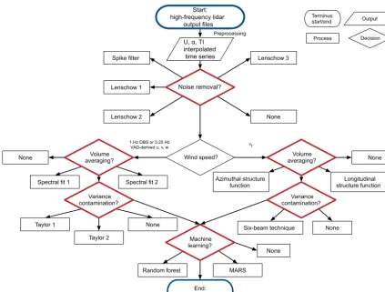
Figure 1.Flowchart depicting different methods for correcting TI with L-TERRA. Starting and ending points are indicated by blue-outlined ovals and modules are indicated by red-outlined diamonds.
|1vi|>2IQR1v,
|1vi−1|>2IQR1v, (7)
1vi 1vi−1
= −1,
where IQR1v is the interquartile range of all values of1v
within the 10 min period. This spike filter eliminates data points defined by a large decrease in velocity followed by a large increase in velocity (or vice versa).
The Lenschow et al. (2000) methods involve the use of the lidar’s velocity spectrum or auto-covariance function to estimate the amount of noise in the variance measurements from the lidar. In the lidar velocity spectrum, power at the high-frequency end of the spectrum is assumed to be largely attributed to white noise. The average power at the high-frequency end of the spectrum is integrated across all fre-quencies to estimate the variance due to noise. An estimate of noise variance can also be made by assuming that noise is random and completely uncorrelated with the velocity signal. Thus, the value of the auto-covariance function at lag 0 is a sum of the noise variance and actual velocity variance. The
noise variance can be estimated by extrapolating the auto-covariance function from non-zero lags to lag 0. The differ-ence between the auto-covariance function at lag 0 and the extrapolated value is the noise variance.
3.2.2 Volume averaging
scan due to the small number of azimuthal angles where data are collected.
Another method of mitigating volume averaging is to model the lidar velocity spectrum and use the model to extrapolate the spectrum to higher frequencies. The high-frequency part of the modeled spectrum can then be inte-grated to obtain an estimate of the variance that is not mea-sured by the lidar as a result of spatial and temporal resolu-tion (e.g., Hogan et al., 2009). The standard Kaimal spectrum used for wind energy (e.g., Burton et al., 2001) requires three parameters for fitting: the mean wind speed, the variance, and a length scale. The first two parameters can be calculated from the lidar data directly, while the last parameter must be estimated. In this work, the length scale was estimated in two different ways: by minimizing the difference between the actual velocity spectrum and the Kaimal spectrum (Spectral Fit 1) and by calculating the integral timescale from the raw velocity time series, which can then be related to the integral length scale through Taylor’s frozen turbulence hypothesis (Spectral Fit 2).
3.2.3 Variance contamination
Methods to reduce variance contamination include the six-beam technique developed by Sathe et al. (2015b), discussed in Sect. 2.3.2, and the use of Taylor’s frozen turbulence hy-pothesis with data from the WC’s vertical beam (Newman, 2015). The six-beam technique can be adapted for the WC DBS scans by estimating the variance from the five differ-ent radial beam positions (four off-vertical and one vertical) and solving a system of five equations to determine the vari-ance and covarivari-ance components. Although the covarivari-ance of theu andv components cannot be determined with this method, the three velocity variance components can be es-timated (Newman et al., 2016b). Taylor’s frozen turbulence hypothesis can be used to relate temporal changes in the ver-tical velocity measured by the WC’s verver-tical beam to spatial changes in the vertical wind field across the WC scanning cir-cle. Spatial changes in thewcomponent can then be used to reduce contamination in either the raw wind speed (Taylor 1) or the variance directly (Taylor 2).
3.3 Machine learning
The last module in L-TERRA uses a trained machine-learning model to further reduce TI error. Inputs for the machine-learning module include lidar-measured parameters (e.g., mean wind speed and shear) and the corrected TI pro-duced by the physics-based corrections. The model must first be trained on one or more datasets that contain data from a collocated met tower and lidar.
Two machine-learning methods were evaluated as part of L-TERRA: random forests and multivariate adaptive regres-sion splines (MARS). The use of other machine-learning techniques such as neural networks could be an area of
fu-ture research, though we decided to focus mainly on the physical corrections for this work. Random forest models are developed by averaging multiple decision trees that were trained on different subsets of the data. By averaging tens or hundreds of decision trees, the variance of the overall model is reduced significantly (Friedman et al., 2001). Ran-dom forests were evaluated because they are relatively easy to understand and have previously been used for wind energy applications (e.g., Clifton et al., 2013; Bulaevskaya et al., 2015). MARS is essentially a stepwise regression model, where different coefficients and basis functions are used to predict the output depending on each region in the dataset (Friedman, 1991). MARS is well-suited for the prediction of physical processes due to its ability to model nonlinearities and interactions among variables.
Potential predictor variables for the machine-learning models were divided into two broad categories: atmospheric state and lidar operating characteristics. Variables that were evaluated as predictor variables in L-TERRA are given in Ta-ble 1. Atmospheric state variaTa-bles included shear parameter, mean wind speed, Doppler spectral broadening, anduandw
velocity variances. Lidar operating characteristics included signal-to-noise ratio (SNR) and internal instrument temper-ature. In all, 18 predictor variables were considered for the machine-learning portion of L-TERRA.
3.4 Comparison to previous methods
In contrast to the methods discussed in Sect. 2.3, L-TERRA uses only information that is available from a standard vertically profiling lidar. The physics-based corrections in L-TERRA require only data from the lidar itself, while the machine-learning module in L-TERRA can be trained using either cup or sonic anemometer data. The majority of the cor-rections in L-TERRA can be implemented with fewer than 20 lines of code, and the models employed in L-TERRA are well-documented in the literature and simple to under-stand. It takes approximately 0.1 s to run L-TERRA for a sin-gle 10 min period, making it easy to implement in real time. As discussed in Sect. 5.1.2, a stability-dependent version of L-TERRA can be used to adapt to changing conditions and apply corrections appropriate for the current atmospheric sta-bility regime.
4 Datasets
4.1 Measurement sites
Figure 2.Inset: Google Earth image of the state of Oklahoma. Location of Southern Great Plains ARM site is denoted by white marker. Larger figure: Google Earth image of the central facility of the Southern Great Plains ARM site (outlined in red box) with overlaid elevation contours in feet. Elevation map is from the United States Geological Survey and uses contour intervals of approximately 10 feet (3.05 m). Locations of WC lidar and 60 m tower are indicated by white markers.
Table 1.Potential predictor variables evaluated in the machine-learning module of L-TERRA.
Potential predictor variables
Atmospheric state Lidar operating characteristics
Original TI SNR
Corrected TI Instrument pitch
σu2 Instrument roll
σw2 Instrument internal temperature
U α
Horizontal wind speed dispersion Vertical wind speed dispersion Spectral broadening
Integral timescale (horizontal) Integral timescale (vertical)
Stationarity (e.g., Vickers and Mahrt, 1997) Maximum instantaneous value ofw Precipitation
measurements at heights corresponding to reference instru-ments.
The ARM site, a field measurement site operated by the US Department of Energy, contains several remote-sensing and in situ instruments (Mather and Voyles, 2013). From November 2012 to June 2013, a WC lidar owned by Lawrence Livermore National Laboratory was deployed at the ARM site approximately 100 m from a 60 m tower. Gill Windmaster Pro 3-D sonic anemometers are mounted on the tower at 25 and 60 m AGL and collect velocity data at a fre-quency of 10 Hz. The ARM site is relatively flat, with max-imum elevation changes of approximately 5 m in the
sur-rounding area. The land to the east of the tower slopes gen-tly upward toward the ARM site (Fig. 2), although few data points from this sector were used to evaluate L-TERRA, as the sonic anemometers are located on the west side of the tower and are thus affected by tower wakes when winds are from this direction.
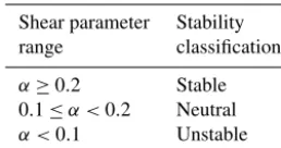
Table 2.Stability classifications used in this work.
Shear parameter Stability range classification
α≥0.2 Stable 0.1≤α <0.2 Neutral α <0.1 Unstable
deployments. The WC was located on the wind farm from November 2013 to July 2014, with a break from February to April 2014 while the WC was deployed for a different field experiment. During the wind farm deployments, the WC was sited in the same enclosure as a met tower with standard wind energy instrumentation, including a cup anemometer at 80 m. For the winter deployment, the WC was located near a met tower on the north end of the wind farm, and for the spring and summer deployment, the WC was moved to a tower en-closure at the south end of the wind farm, in accordance with the dominant wind direction during each season at the wind farm. Directional sectors that may have been influenced by nearby turbines were determined following the guidelines in Annex A of IEC 61400-12-1 (International Electrotechnical Commission, 2013) and were excluded from the dataset.
4.2 Stability classification
Typical atmospheric stability parameters include the gradi-ent Richardson number (Ri) and the Monin–Obukhov length (L) (e.g., Stull, 2000). The calculation ofRirequires temper-ature and wind speed measurements at two different heights, while the calculation ofLrequires high-frequency flux mea-surements at a single height. As the goal of L-TERRA is to apply TI corrections to a stand-alone lidar, we preferred to classify stability depending only on measurements available from a lidar.
One option for a lidar-based stability parameter is the shear exponent, α (Eq. 4). Although α can change with height or surface roughness (e.g., Petersen et al., 1998), it is strongly tied to the atmospheric stability in the Central and Southern Plains regions of the United States (e.g., Wal-ter et al., 2009; Vanderwende and Lundquist, 2012; Newman and Klein, 2014). This relation is likely apparent because the diurnal transition of the atmospheric boundary layer largely controls the wind speed profile in flat terrain (e.g., Arya, 2001).
To test the ability of the lidar shear exponent to classify stability, values of α calculated with WC data between 40 and 200 m were compared to values ofRicalculated from 4 and 60 m wind speed and temperature data from the ARM site. Ri was estimated with the following equation (Bodine et al., 2009; Newman and Klein, 2014):
Ri=g[(T60 m−T4 m)/1zT+0d]1z 2
U T4 m(U60 m−U4 m)2
, (8)
Figure 3.Richardson number from tower data at the ARM site vs. shear exponent calculated from WC data. Dashed lines denote sta-bility thresholds as defined in the text. Magenta, green, and blue circles correspond to times when the classification based on both Riandαwas unstable, neutral, or stable, respectively, and gray cir-cles correspond to times when the classification was different. Open gray circles denote times when the classification was stable based onRiand unstable based onαor vice versa. Percentages of the to-tal combinedRi–αdataset corresponding to each case are shown in parentheses in the figure legend.
where g (m s−2) denotes the gravitational acceleration, T
(K) is the temperature, U (m s−1) is the mean horizontal wind speed,0d(K m−1) is the dry adiabatic lapse rate, and 1zT and1zU (m) represent the difference in measurement
height for values ofT andU, respectively. Thresholds for
αare loosely based on the thresholds used in Wharton and Lundquist (2012) and are given in Table 2. Thresholds forRi were−0.17 for the transition between unstable and neutral conditions and 0.06 for the transition between neutral and stable conditions, as in Vanderwende and Lundquist (2012).
A scatterplot ofRiversusαfor the ARM site is shown in Fig. 3. (Only 30 min temperature data were available from the tower, so 30 min, rather than 10 min, values ofRiandα
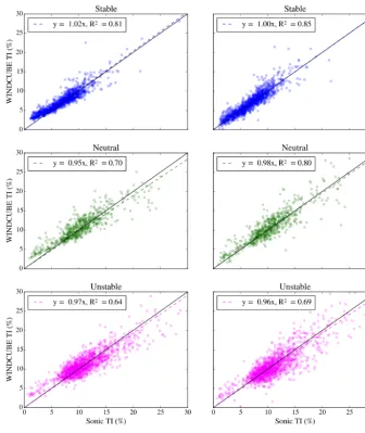
Figure 4.Scatterplots of met tower vs. WC TI for data from 60 m measurement height at the ARM site(a)before and(b)after L-TERRA-S has been applied. The 1 : 1 line and regression lines are shown for reference, and regression line statistics are shown in figure legends.
4.3 Comparison of mean wind speed and TI
At both sites, 10 min mean wind speeds measured by the WC and the met tower instruments were well-correlated, with re-gression line slopes of approximately 1 andR2values of ap-proximately 0.99 (not shown). Thus, we felt confident that the WC was measuring similar conditions to the reference instruments, though a modified version of L-TERRA could be used in the future to mitigate any small errors in mea-surement of mean wind speeds. Larger discrepancies were evident in the comparison of TI values, which is our current area of focus for L-TERRA. Sample scatterplots of met tower versus lidar TI for the ARM site are shown in Fig. 4a, and
corresponding regression statistics for the raw TI are shown in Table 3.
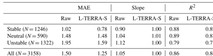
Table 3.Mean absolute error (MAE) and slope andR2values of regression lines for WC TI compared to met tower TI before and after L-TERRA-S has been applied for the 60 m measurement height at the ARM site.
MAE Slope R2
Raw L-TERRA-S Raw L-TERRA-S Raw L-TERRA-S
Stable (N=1246) 1.02 0.78 0.90 1.00 0.88 0.89 Neutral (N=590) 1.48 1.48 1.04 1.01 0.89 0.87 Unstable (N=1322) 1.95 1.59 1.12 1.00 0.79 0.77
All (N=3158) 1.50 1.25 1.05 1.00 0.86 0.86
that classified lidar variance errors by stability, we felt confi-dent in usingαas a proxy for stability for the datasets in this work.
5 L-TERRA results
First, data from each site were examined individually to as-sess the performance of L-TERRA. Results from the physics-based corrections were analyzed separately from results from the full version of L-TERRA (physics-based corrections plus machine learning) to assess how well each set of corrections performed.
5.1 Application of physics-based corrections 5.1.1 Initial version of L-TERRA
For both the ARM site and the wind farm, all possible combinations of the physics-based corrections described in Sect. 3.2 for theu,v, andwcomponents were evaluated. Ini-tially, the model combination that minimized the overall TI MAE was selected as the optimal model combination for that particular site. Data were filtered to avoid mast shadowing, and 10 min periods where the mean wind speed was less than 4 m s−1were not used to evaluate L-TERRA, as the standards outlined in IEC 61400-12-1 (International Electrotechnical Commission, 2013) restrict remote-sensing classification to wind speeds between 4 and 16 m s−1.
At the ARM site, the original TI MAE was 1.5 %, and MAE values that resulted from the application of L-TERRA ranged from 1.31 to 2.73 %. MAE values above the origi-nal value of 1.5 % indicate that for these model combina-tions, L-TERRA actually increased overall error in WC TI. For many of these model combinations with high MAE val-ues, the MAE increased for stable conditions, while decreas-ing for unstable conditions and vice versa, indicatdecreas-ing that some model combinations work better for particular stabil-ity conditions than others. Many of the high MAE values were also associated with model combinations that used the Lenschow noise removal techniques with the 4 s VAD scans. The Lenschow techniques are more aggressive with noise re-moval than a spike filter and also involve directly reducing the variance due to noise, rather than removing spikes in the
raw velocity time series. It is possible that the noise appar-ent in the original WC data artificially brought the WC TI estimates closer to the sonic TI, and removing the noise vari-ance decreased the WC TI values, bringing them further from the sonic values and increasing the MAE. In addition, spec-tra and auto-covariance functions derived from the 4 s data are expected to be less accurate than those derived from the higher-resolution 1 s data, which could affect the accuracy of the Lenschow techniques.
TI MAE values also varied a large amount at the wind farm, with an original MAE of 1.46 % and L-TERRA MAE values ranging from 1.38 to 2.9 %. Similarly to the ARM site, many of the higher MAE values were associated with model combinations that decreased the MAE for certain sta-bility conditions while increasing the MAE for other stasta-bility conditions.
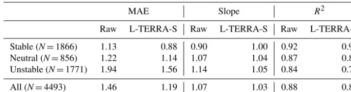
Table 4.As in Table 3 but for Southern Plains wind farm data.
MAE Slope R2
Raw L-TERRA-S Raw L-TERRA-S Raw L-TERRA-S
Stable (N=1866) 1.13 0.88 0.90 1.00 0.92 0.92 Neutral (N=856) 1.22 1.14 1.07 1.04 0.87 0.85 Unstable (N=1771) 1.94 1.56 1.14 1.05 0.84 0.78
All (N=4493) 1.46 1.19 1.07 1.03 0.88 0.87
and provides a useful baseline combination for evaluating L-TERRA.
5.1.2 Stability-dependent version of L-TERRA
By examining the change in lidar TI after each step in L-TERRA, it was determined that some corrections de-creased error under stable conditions but inde-creased error un-der unstable conditions and vice versa. This is not surpris-ing, as the magnitude and sign of TI errors was strongly de-pendent on atmospheric stability at both sites (Tables 3, 4) as a result of the different factors that affect TI error under different stability conditions. Thus, optimal model combina-tions were next determined separately for the three different bulk stability classes to form a stability-dependent version of L-TERRA (L-TERRA-S). Optimal model combinations were very similar for both sites and are shown in Table 5.
For stable and unstable conditions, a spike filter was the optimal noise removal technique. Only the model chain for stable conditions included a volume averaging correction, likely because volume averaging effects on TI are largest under stable conditions. For unstable conditions, using the velocity time series from the VAD technique produced the largest reduction in MAE. While the raw output time series from the WC is available at 1 Hz (Sect. 2.1), the VAD tech-nique is typically applied once per full scan to derive the three-dimensional wind vector. For the WC, this results in an output data frequency of 0.25 Hz for the VAD technique. The lower temporal resolution of the VAD technique likely served to artificially reduce some of the effects of variance contamination, as smaller scales of turbulence were not mea-sured.
The impact of each of the different physics-based correc-tion modules on the TI error is shown in Fig. 5. Overall, MAE steadily decreased after the application of the different cor-rections, with the largest decrease occurring for the volume averaging module. For unstable TI values, the noise reduc-tion module had the largest impact on reducing MAE and bringing the regression line slope closer to 1. The variance contamination module served to further reduce the MAE and regression line slope, bringing the slope from approxi-mately 1.05 to 1.00, but theR2 value of the regression line decreased. Similarly, the variance contamination module re-duced the regression line slope for neutral TI values, bringing
it closer to 1, but caused theR2value of the regression line to decrease. This resulted in an MAE value of 1.48 % for neu-tral TI values after L-TERRA was applied, which is the same as the original MAE value for neutral conditions. The cor-rections performed best on stable TI values, with MAE val-ues steadily decreasing andR2values increasing with each correction. The volume averaging module caused the largest change in stable TI values, with the regression line slope in-creasing from 0.90 to 1.01 after the application of the volume averaging module. In summary, all the physics-based correc-tions in L-TERRA appear necessary to the correction of WC TI, though the importance of each correction depends on the stability. The variance contamination module likely needs to be improved for certain types of unstable and neutral condi-tions, as it increased TI error for some unstable and neutral TI values.
Scatterplots of ARM site TI data after L-TERRA-S was applied are shown in Fig. 4b, and corresponding regression statistics are shown in Table 3. L-TERRA-S served to bring the majority of WC TI estimates closer to the 1 : 1 line, re-sulting in regression line slopes of 1.00, 1.01, and 1.00 for stable, neutral, and unstable conditions, respectively. In ad-dition, the overall TI MAE decreased from 1.5 to 1.25 %. However, as discussed in the previous paragraph,R2values for neutral and unstable conditions decreased slightly. Thus, although L-TERRA-S improved the accuracy of most lidar TI estimates, it also increased scatter for neutral and unstable conditions.
Results for the wind farm were similar, with overall MAE decreasing from 1.46 to 1.19 % and regression line slopes be-coming 1.00, 1.04, and 1.05 for stable, neutral, and unstable conditions, respectively (Table 4).R2values for neutral and unstable conditions also decreased slightly.
5.1.3 Effects of stability misclassification
Table 5.L-TERRA model combinations that minimized TI MAE for different stability conditions at the ARM site and Southern Plains wind farm.
Stability Wind speed Noise Volume Variance classification frequency averaging contamination
All 1 Hz Lenschow 1 None Taylor 2
Stable 1 Hz Spike filter Spectral Fit 2 Taylor 1
Neutral 1 Hz None None Taylor 2
Unstable 0.25 Hz Spike filter None Taylor 1
Figure 5.Progression of MAE (top), regression line slope (middle), andR2value of regression line (bottom) for WC vs. sonic TI at the ARM site after the application of different modules in L-TERRA-S.
TI. To examine the impact of incorrect stability classification on remaining TI errors, time periods were identified where the WC TI error at the ARM site was above the 95th per-centile of all TI errors after L-TERRA-S was applied; these TI values represent outliers in Fig. 4b and contribute signifi-cantly to the low values ofR2.
Of the 56 TI outliers identified that were associated with valid values ofRiandα, 16 points were classified as unstable by bothRiandα, 5 points were classified as neutral by both parameters, and 4 points were classified as stable by both pa-rameters. The remaining 33 points were classified differently byRiandα, with nearly half (14) of the points being
classi-fied as neutral byRiand slightly unstable or slightly stable byα, 12 points being classified as stable or unstable byRi and neutral byα, and the remaining 5 points being classified as stable byRiand slightly unstable by α. The majority of these stability misclassifications appear to occur near neutral conditions, where small errors in measurement of the wind shear or temperature gradient could lead to a different stabil-ity classification. Thus, it may be useful in the future to use a blend of correction techniques for points classified as near-neutral or use additional parameters to classify stability from lidar data. However, as opposing stability classifications ac-counted for fewer than 10 % of the large TI errors apparent after the application of L-TERRA-S, it is likely that other factors were also responsible for the large amount of scat-ter still apparent in the TI data. For example, it is likely that the current physics-based corrections in L-TERRA-S do not fully capture all the factors that affect lidar TI error, result-ing in large errors that remain for some data points. In the next section, machine-learning techniques are evaluated as a potential method to model the remaining physics that impact lidar TI error.
5.2 Application of machine-learning techniques
The physics-based corrections described in the previous sec-tion require only data from the lidar itself and do not require any training data. In contrast, machine-learning models must be trained on a dataset before being applied to new data. Typically, a single dataset is split into training and testing datasets in a method known as cross validation (e.g., Efron and Gong, 1983) to test the accuracy of the model on data that was not included in the training process. As the end goal of L-TERRA is to provide accurate lidar TI values at a site that does not have a met tower, the machine-learning model in L-TERRA must be trained on one or more sites with a met tower before being applied to a lidar at a new site. Thus, the machine-learning models discussed in this section were trained on the wind farm data and then applied to data from the ARM site for validation.
5.2.1 Determination of predictor variables
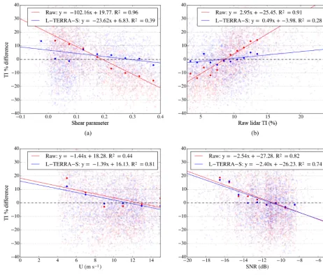
con-Figure 6.Percent difference between WC and sonic TI for the ARM site as a function of(a)shear parameter,(b)raw WC TI,(c)mean wind speed, and(d)SNR. Differences are shown both before (red circles) and after (blue circles) L-TERRA-S has been applied. Solid circles correspond to averages of binned data and solid lines correspond to regression line fits to bin means, following the procedure in Annex L of IEC 61400-12-1, Draft Edition (International Electrotechnical Commission, 2013).
ducted for the WC TI error at both sites. The sensitivity of the lidar TI error to the various predictor variables in Table 1 was quantified following the guidelines in Annex L of the new committee draft of IEC 61400-12-1 (International Elec-trotechnical Commission, 2013). First, predictor variables were binned and bin means of the TI percent error corre-sponding to each bin were calculated. A least-squares tech-nique was then used to calculate a regression line between the predictor bin centers and the bin means of the TI percent error. Sensitivity, defined as the product of the regression line slope and the standard deviation of the predictor variable, was then calculated for each predictor. The sensitivity gives the approximate change in the TI error for a change in the predictor variable that is equivalent to 1 standard deviation of the variable.
Figure 7.Scatterplots of met tower vs. WC TI for data from 60 m measurement height at the ARM site(a)after the application of the first random forest described in the text and(b)after the application of the second random forest. The 1 : 1 line and regression lines are shown for reference.
Overall, the six variables for the ARM site with the highest sensitivity values after the application of L-TERRA-S were as follows: integral timescale (vertical), SNR, corrected TI, integral timescale (horizontal), mean wind speed, and shear parameter. (For highly correlated variables, the variable with a higher sensitivity was retained in the list.) These six vari-ables were then used to train a random forest with the wind farm data.
5.2.2 Results from trained machine-learning model Results from the application of the trained random forest on the ARM site L-TERRA-S TI values are shown in Fig. 7a. The application of the random forest increased MAE values from 0.78 to 0.89 % for stable conditions and from 1.48 to 1.6 % for neutral conditions and decreased the MAE from
1.59 to 1.53 % for unstable conditions in comparison to the results from L-TERRA-S. For all three stability classifica-tions,R2values dropped significantly and a positive bias was induced for low TI values.
re-lated to the different sensitivities associated with two of the input parameters. However, even with these two parameters removed from the input parameter list, the MAE values still increased in comparison to L-TERRA-S, whileR2values de-creased. Results from the MARS model were similar to those from the random forest models.
These results highlight two major limitations of using machine-learning techniques to improve lidar TI accuracy in L-TERRA: (1) the most significant input parameters can change from one site to another and will not be known a pri-ori for a new site, and (2) the sensitivity of TI error to dif-ferent input variables depends on the training site and the particular lidar and reference measurements used. To inves-tigate the effect of the training dataset used, a random forest was also trained on 75 % of the ARM site data and then ap-plied to the remaining 25 %. Training and testing a random forest on data from the same site did decrease MAE values in comparison to results from L-TERRA-S, butR2values still decreased slightly for neutral and unstable conditions. More importantly, using this technique would preclude L-TERRA from being applied at a new site that does not have a met tower.
Although machine learning can be a useful tool for turbine power prediction (e.g., Clifton et al., 2013), it does not appear to be an ideal technique for correcting lidar TI error. Thus, the next steps in the development of L-TERRA will involve further refining the physics-based corrections in L-TERRA-S to improve TI estimates in a more robust manner. Rather than relying on modeled patterns, physics-based corrections di-rectly relate lidar measurements to TI errors and substantially improved the accuracy of lidar TI estimates at both sites eval-uated in this work (Fig. 4, Tables 3 and 4). However, the cur-rent physics-based corrections do not completely eliminate TI error, indicating that the physics that cause TI error are not being entirely captured in L-TERRA-S. Future work will in-volve the development of a lidar uncertainty framework that outlines all possible causes of lidar error. Different parts of the framework could then be quantified through the use of a simulated flow field and virtual lidar, as in Lundquist et al. (2015).
Results from the sensitivity analysis conducted in this sec-tion will greatly assist in determining areas of focus for the lidar uncertainty framework. For example, TI error at both sites was extremely sensitive to the integral timescale of the
wwind component, which is a proxy for the dominant tem-poral scale of turbulent eddies in the vertical direction. Thus, lidar TI error appears to be strongly affected by the scales of vertical motion present in the area enclosed by the lidar scanning circle, which will contribute to the degree of vari-ance contamination. Currently, no physical models exist that could account for these effects, and so we suggest that this could be a fruitful research direction. In future work, the vir-tual lidar tool will be used to examine how changes in the vertical flow field across the lidar scanning circle impact TI
estimates and how information from the lidar can be used to approximate and remove these effects.
6 Conclusions and future work
Lidars are currently being considered as a replacement for meteorological towers in the wind energy industry. Unlike met towers, lidars can be easily deployed at different loca-tions and are capable of collecting wind speed measurements at heights spanning the entire turbine rotor disk. However, lidars measure different values of TI than a cup or sonic anemometer, and this uncertainty in lidar TI estimates is a major barrier to the adoption of lidars for wind resource as-sessment and power performance testing. In this work, a li-dar turbulence error reduction model, L-TERRA, was devel-oped and tested on WC lidar data from two different sites. The model incorporates both physics-based corrections and machine-learning techniques to improve lidar TI estimates.
The main findings from this work can be summarized as follows:
– The difference between TI measured by a cup or sonic anemometer and that measured by a vertically profiling lidar can be reduced using appropriate physical models of the lidar measurements.
– Performance of L-TERRA improves substantially when different model configurations are used for different sta-bility conditions (i.e., in L-TERRA-S).
– In addition to reducing MAE, L-TERRA-S also reduces the sensitivity of lidar TI error to atmospheric stability.
– The accuracy of a machine-learning method in L-TERRA-S is highly dependent on the sensitivity of the lidar TI error to the input parameters at both the training and testing sites.
Further improvements to L-TERRA-S can be made through a better understanding of how atmospheric conditions and lidar operating characteristics impact TI error. This understanding can be achieved through the development of a lidar uncer-tainty framework and testing of the framework with mod-eled atmospheric data. Future work on L-TERRA-S will also include testing with additional datasets, including datasets from complex terrain and different areas of the world. Practi-cal applications of L-TERRA for site assessment and power prediction will also be explored in future work.
could also help wind energy developers make more informed decisions about turbine selection and wind farm layout. The use of lidars in place of met towers for wind energy appli-cations should allow for a more rapid development of wind in regions where it is difficult or costly to install met tow-ers, and the improvement of lidar turbulence estimates will greatly assist in the adoption of lidars in the wind industry.
7 Data availability
Mean sonic anemometer wind speed data from the 60 m tower at the ARM site are publicly available at https:// www.arm.gov/capabilities/instruments/co2flx (ARM, 2011) and mean temperature data from the temperature probes on the tower can be found at https://www.arm.gov/ capabilities/instruments/twr (ARM, 1993). High-frequency sonic anemometer and lidar data are available upon re-quest ([email protected]). Meteorological tower data from the wind farm cannot be shared per a nondisclo-sure agreement with the wind farm.
Competing interests. The authors declare that they have no con-flict of interest.
Acknowledgements. The authors would like to thank the staff of the Southern Great Plains ARM site and the Southern Plains wind farm for assisting with the lidar field deployments. Sebastien Bi-raud and Marc Fischer of Lawrence Berkeley National Laboratory supplied sonic anemometer data for the ARM site. Sonia Wharton of Lawrence Livermore National Laboratory provided the WIND-CUBE lidar used in this work and assisted with field deploy-ments. Leosphere and NRG Systems provided technical support for the WINDCUBE lidar during the experiments. Conversations with Caleb Phillips at NREL greatly enhanced our understanding of dif-ferent machine-learning models. We also thank Rozenn Wagner and an anonymous reviewer whose comments helped improve the paper. The ARM Climate Research Facility is a US Department of Energy Office of Science user facility sponsored by the Office of Biological and Environmental Research. This work was supported by the US Department of Energy under contract no. DE-AC36-08GO28308 with the National Renewable Energy Laboratory. Funding for the work was provided by the DOE Office of Energy Efficiency and Renewable Energy, Wind and Water Power Technologies Office.
The US Government retains and the publisher, by accepting the article for publication, acknowledges that the US Government retains a nonexclusive, paid-up, irrevocable, worldwide license to publish or reproduce the published form of this work, or allow others to do so, for US Government purposes.
Edited by: J. Mann
Reviewed by: R. Wagner and one anonymous referee
References
ARM (Atmospheric Radiation Measurement): Climate Research Facility, updated daily, Facility-specific multi-level mete-orological instrumentation (TWR), Nov. 2012–Jun. 2013, 36◦36018.000N, 97◦2906.000W: Southern Great Plains Cen-tral Facility (C1), compiled by: Cook, D. and Kyrouac, J., ARM Data Archive: Oak Ridge, Tennessee, USA, available at: https://www.arm.gov/capabilities/instruments/twr (last ac-cess: 11 April 2013), 1993.
ARM (Atmospheric Radiation Measurement): Climate Research Facility, updated daily, Carbon dioxide flux measurement systems (CO2FLX), Nov. 2012–Jun. 2013, 36◦36018.000N, 97◦2906.000W: Southern Great Plains Central Facility (C1), compiled by: Billesbach, D., Biraud, S., and Chan, S., ARM Data Archive: Oak Ridge, Tennessee, USA, available at: https://www.arm.gov/capabilities/instruments/co2flx (last ac-cess: 11 April 2013), 2011.
Arya, S. P.: Introduction to Micrometeorology, Academic Press, Cornwall, UK, 2nd Edn., Int. Geophys. Ser., 79, 101–108, 2001. Barthelmie, R. J., Crippa, P., Wang, H., Smith, C. M., Krishna-murthy, R., Choukulkar, A., Calhoun, R., Valyou, D., Marzocca, P., Matthiesen, D., Brown, G., and Pryor, S. C.: 3D wind and turbulence characteristics of the atmospheric boundary layer, Bull. Amer. Meteor. Soc., 95, 743–756, doi:10.1175/BAMS-D-12-00111.1, 2013.
Bodine, D., Klein, P. M., Arms, S. C., and Shapiro, A.: Variabil-ity of surface air temperature over gently sloped terrain, J. Appl. Meteor. Climatol., 48, 1117–1141, 2009.
Boquet, M., Callard, P., Deve, N., and Osler, E.: Return on invest-ment of a lidar remote sensing device, DEWI Magazine, 37, 56– 61, 2010.
Branlard, E., Pedersen, A. T., Mann, J., Angelou, N., Fischer, A., Mikkelsen, T., Harris, M., Slinger, C., and Montes, B. F.: Re-trieving wind statistics from average spectrum of continuous-wave lidar, Atmos. Meas. Tech., 6, 1673–1683, doi:10.5194/amt-6-1673-2013, 2013.
Browning, K. A. and Wexler, R.: The determination of kinematic properties of a wind field using Doppler radar, J. Appl. Meteor., 7, 105–113, doi:10.1175/1520-0450(1968)007<0105:TDOKPO>2.0.CO;2, 1968.
Bulaevskaya, V., Wharton, S., Clifton, A., Qualley, G., and Miller, W. O.: Wind power curve modeling in complex terrain using sta-tistical models, Journal of Renewable and Sustainable Energy, 7, 013103, doi:10.1063/1.4904430, 2015.
Burton, T., Sharpe, D., Jenkins, N., and Bossanyi, E.: Wind Energy Handbook, John Wiley & Sons, Ltd., 2001.
Calhoun, R., Heap, R., Princevac, M., Newsom, R., Fernando, H., and Ligon, D.: Virtual towers using coherent Doppler lidar dur-ing the Joint Urban 2003 Dispersion Experiment, J. Appl. Me-teor., 45, 1116–1126, doi:10.1175/JAM2391.1, 2006.
Chang, W. S.: Principles of Lasers and Optics, Cambridge Univer-sity Press, 2005.
Clifton, A. and Wagner, R.: Accounting for the effect of turbulence on wind turbine power curves, J. Phys. Conf. Ser., 524, 012109, doi:10.1088/1742-6596/524/1/012109, 2014.
Clifton, A., Boquet, M., Roziers, E. B. D., Westerhellweg, A., Hof-säß, M., Klaas, T., Vogstad, K., Clive, P., Harris, M., Wylie, S., Osler, E., Banta, B., Choukulkar, A., Lundquist, J., and Aitken, M.: Remote sensing of complex flows by Doppler wind lidar: Is-sues and preliminary recommendations, Tech. Rep. NREL/TP-5000-64634, NREL, http://www.nrel.gov/docs/fy16osti/64634. pdf (last access: 3 February 2017), 2015.
Efron, B. and Gong, G.: A leisurely look at the bootstrap, the jack-knife, and cross-validation, Am. Stat., 37, 36–48, 1983. Elliott, D. L. and Cadogan, J. B.: Effects of wind shear and
turbu-lence on wind turbine power curves, in: European Community Wind Energy Conference and Exhibition, Madrid, Spain, 1990. Emeis, S.: Measurement Methods in Atmospheric Sciences: In-Situ
and Remote, Borntraeger Science Publishers, 257 pp., 2010. Friedman, J., Hastie, T., and Tibshirani, R.: The Elements of
Sta-tistical Learning, Springer Series in Statistics Springer, Berlin, Vol. 1, 587–604, 2001.
Friedman, J. H.: Multivariate adaptive regression splines, Ann. Stat., 19, 1–67, 1991.
Fuertes, F. C., Iungo, G. V., and Porté-Agel, F.: 3D turbulence measurements using three synchronous wind lidars: Validation against sonic anemometry, J. Atmos. Ocean. Tech., 31, 1549– 1556, doi:10.1175/JTECH-D-13-00206.1, 2014.
Hogan, R. J., Grant, A. L., Illingworth, A. J., Pearson, G. N., and O’Connor, E. J.: Vertical velocity variance and skewness in clear and cloud-topped boundary layers as revealed by Doppler lidar, Q. J. Roy. Meteor. Soc., 135, 635–643, doi:10.1002/qj.413, 2009. Huffaker, R. M. and Hardesty, R. M.: Remote sensing of atmo-spheric wind velocities using solid-state and CO2coherent laser
systems, P. IEEE, 84, 181–204, 1996.
International Electrotechnical Commission: Wind turbines – Part 1: Design requirements, Tech. Rep., IEC 61400-1, Geneva, Switzer-land, 2005.
International Electrotechnical Commission: Wind turbines – Part 12-1: Power performance measurements of electricity producing wind turbines, Tech. Rep. Committee draft Edn., IEC 61400-12-1, Geneva, Switzerland, 2013.
Kaimal, J. and Finnigan, J.: Atmospheric Boundary Layer Flows: Their Structure and Measurement, Oxford University Press, 1994.
Kolmogorov, A. N.: The local structure of turbulence in incom-pressible viscous fluid for very large Reynolds numbers, Doklady AN SSSR, 30, 301–304, 1941.
Krishnamurthy, R., Calhoun, R., Billings, B., and Doyle, J.: Wind turbulence estimates in a valley by coherent Doppler lidar, Mete-orol. Appl., 18, 361–371, doi:10.1002/met.263, 2011.
Krishnamurthy, R., Choukulkar, A., Calhoun, R., Fine, J., Oliver, A., and Barr, K.: Coherent Doppler lidar for wind farm character-ization, Wind Energy, 16, 189–206, doi:10.1002/we.539, 2013. Lenschow, D. H., Wulfmeyer, V., and Senff, C.:
Measur-ing second-through fourth-order moments in noisy data, J. Atmos. Ocean. Tech., 17, 1330–1347, doi:10.1175/1520-0426(2000)017<1330:MSTFOM>2.0.CO;2, 2000.
Lundquist, J. K., Churchfield, M. J., Lee, S., and Clifton, A.: Quan-tifying error of lidar and sodar Doppler beam swinging measure-ments of wind turbine wakes using computational fluid dynam-ics, Atmos. Meas. Tech., 8, 907–920, doi:10.5194/amt-8-907-2015, 2015.
Mann, J.: The spatial structure of neutral atmospheric surface-layer turbulence, J. Fluid Mech., 273, 141–168, doi:10.1017/S0022112094001886, 1994.
Mann, J., Peña, A., Bingöl, F., Wagner, R., and Courtney, M. S.: Lidar scanning of momentum flux in and above the atmo-spheric surface layer, J. Atmos. Ocean. Tech., 27, 959–976, doi:10.1175/2010JTECHA1389.1, 2010.
Mather, J. H. and Voyles, J. W.: The ARM Climate Research Facil-ity: A review of structure and capabilities, Bull. Amer. Meteor. Soc., 94, 377–392, doi:10.1175/BAMS-D-11-00218.1, 2013. Newman, J. F.: Optimizing lidar scanning strategies for wind energy
turbulence measurements, Ph.D. thesis, University of Oklahoma, Norman, Oklahoma, USA, 2015.
Newman, J. F. and Klein, P. M.: The impacts of atmospheric sta-bility on the accuracy of wind speed extrapolation methods, Re-sources, 3, 81–105, doi:10.3390/resources3010081, 2014. Newman, J. F., Bonin, T. A., Klein, P. M., Wharton, S., and
New-som, R. K.: Testing and validation of multi-lidar scanning strate-gies for wind energy applications, Wind Energy, 19, 2239–2254, doi:10.1002/we.1978, 2016a.
Newman, J. F., Klein, P. M., Wharton, S., Sathe, A., Bonin, T. A., Chilson, P. B., and Muschinski, A.: Evaluation of three lidar scanning strategies for turbulence measurements, Atmos. Meas. Tech., 9, 1993–2013, doi:10.5194/amt-9-1993-2016, 2016b. Newsom, R. K., Berg, L. K., Shaw, W. J., and Fischer, M. L.:
Turbine-scale wind field measurements using dual-Doppler lidar, Wind Energy, 18, 219–235, doi:10.1002/we.1691, 2015. Peinke, J., Barth, S., Böttcher, F., Heinemann, D., and Lange, B.:
Turbulence, a challenging problem for wind energy, Physica A, 338, 187–193, 2004.
Peña, A., Hasager, C. B., Gryning, S.-E., Courtney, M., Antoniou, I., and Mikkelsen, T.: Offshore wind profiling using light de-tection and ranging measurements, Wind Energy, 12, 105–124, doi:10.1002/we.283, 2009.
Petersen, E. L., Mortensen, N. G., Landberg, L., Højstrup, J., and Frank, H. P.: Wind power meteorology, Part I: Climate and tur-bulence, Wind Energy, 1, 25–45, 1998.
Rodrigo, J. S., Guillén, F. B., Arranz, P. G., Courtney, M., Wagner, R., and Dupont, E.: Multi-site testing and evaluation of remote sensing instruments for wind energy applications, Renew. Energ., 53, 200–210, doi:10.1016/j.renene.2012.11.020, 2013.
Sathe, A. and Mann, J.: A review of turbulence measurements using ground-based wind lidars, Atmos. Meas. Tech., 6, 3147–3167, doi:10.5194/amt-6-3147-2013, 2013.
Sathe, A., Mann, J., Gottschall, J., and Courtney, M. S.: Can wind lidars measure turbulence?, J. Atmos. Ocean. Tech., 28, 853–868, doi:10.1175/JTECH-D-10-05004.1, 2011.
Sathe, A., Mann, J., Barlas, T., Bierbooms, W. A. A. M., and van Bussel, G. J. W.: Influence of atmospheric stability on wind tur-bine loads, Wind Energy, 16, 1013–1032, doi:10.1002/we.1528, 2013.
Sathe, A., Banta, R., Pauscher, L., Vogstad, K., Schlipf, D., and Wylie, S.: Estimating turbulence statistics and parameters from ground- and nacelle-based lidar measurements: IEA Wind expert report, DTU Wind Energy, Denmark, 2015a.
Schneemann, J., Voss, S., Steinfeld, G., Trabucchi, D., Trujillo, J. J., Witha, B., and Kühn, M.: Lidar simulations to study mea-surements of turbulence in different atmospheric conditions, in: Wind Energy – Impact of Turbulence, Springer Berlin Heidel-berg, Berlin, HeidelHeidel-berg, 127–132, 2014.
Sjöholm, M., Mikkelsen, T., Mann, J., Enevoldsen, K., and Court-ney, M.: Time series analysis of continuous-wave coherent Doppler lidar wind measurements, IOP C. Ser. Earth Env., 1, 012051, doi:10.1088/1755-1307/1/1/012051, 2008.
Sjöholm, M., Mikkelsen, T., Mann, J., Enevoldsen, K., and Court-ney, M.: Spatial averaging-effects on turbulence measured by a continuous-wave coherent lidar, Meteor. Z., 18, 281–287, doi:10.1127/0941-2948/2009/0379, 2009.
Slinger, C. and Harris, M.: Introduction to continuous-wave Doppler lidar, in: Summer School in Remote Sensing for Wind Energy, Boulder, CO, 2012.
Sonnenschein, C. M. and Horrigan, F. A.: Signal-to-noise relationships for coaxial systems that heterodyne backscat-ter from the atmosphere, Appl. Opt., 10, 1600–1604, doi:10.1364/AO.10.001600, 1971.
Stawiarski, C., Träumner, K., Knigge, C., and Calhoun, R.: Scopes and challenges of dual-Doppler lidar wind measurements – An error analysis, J. Atmos. Ocean. Tech., 30, 2044–2062, doi:10.1175/JTECH-D-12-00244.1, 2013.
Strauch, R. G., Merritt, D. A., Moran, K. P., Earnshaw, K. B., and De Kamp, D. V.: The Colorado wind-profiling net-work, J. Atmos. Ocean. Tech., 1, 37–49, doi:10.1175/1520-0426(1984)001<0037:TCWPN>2.0.CO;2, 1984.
Stull, R. B.: Meteorology for Scientists and Engineers, Brooks/Cole, 2nd Edn., 2000.
Vanderwende, B. J. and Lundquist, J. K.: The modification of wind turbine performance by statistically distinct atmospheric regimes, Environ. Res. Lett., 7, 034035, doi:10.1088/1748-9326/7/3/034035, 2012.
Vasiljevic, N., Courtney, M., and Mann, J.: A time-space synchro-nization of coherent Doppler scanning lidars for 3D measure-ments of wind fields, PhD thesis, Denmark Technical University, Denmark, 2014.
Vickers, D. and Mahrt, L.: Quality control and flux sam-pling problems for tower and aircraft data, J. At-mos. Ocean. Tech., 14, 512–526, doi:10.1175/1520-0426(1997)014<0512:QCAFSP>2.0.CO;2, 1997.
Wagner, R., Antoniou, I., Pedersen, S. M., Courtney, M. S., and Jørgensen, H. E.: The influence of the wind speed profile on wind turbine performance measurements, Wind Energy, 12, 348–362, doi:10.1002/we.297, 2009.
Wainwright, C. E., Stepanian, P. M., Chilson, P. B., Palmer, R. D., Fedorovich, E., and Gibbs, J. A.: A time series sodar simulator based on large-eddy simulation, J. Atmos. Ocean. Tech., 31, 876– 889, doi:10.1175/JTECH-D-13-00161.1, 2014.
Walter, K., Weiss, C. C., Swift, A. H., Chapman, J., and Kel-ley, N. D.: Speed and direction shear in the stable nocturnal boundary layer, J. Sol. Energ.-T. Asme, 131, 11013–11013, doi:10.1115/1.3035818, 2009.
Wang, H., Barthelmie, R. J., Clifton, A., and Pryor, S. C.: Wind measurements from arc scans with Doppler wind lidar, J. At-mos. Ocean. Tech., 32, 2024–2040, doi:10.1175/JTECH-D-14-00059.1, 2015.
Weitkamp, C.: Lidar: Range-Resolved Optical Remote Sensing of the Atmosphere, Springer Series in Optical Sciences, Springer Science & Business Media, 102, 325–354, 2005.
Wharton, S. and Lundquist, J. K.: Assessing atmospheric stability and its impacts on rotor-disk wind characteristics at an onshore wind farm, Wind Energy, 15, 525–546, doi:10.1002/we.483, 2012.
Wharton, S., Newman, J. F., Qualley, G., and Miller, W. O.: Measuring turbine inflow with vertically-profiling lidar in com-plex terrain, J. Wind Eng. Ind. Aerodyn., 142, 217–231, doi:10.1016/j.jweia.2015.03.023, 2015.