The Influence of the Planets, Sun and Moon on the
Evolution of the Earth’s Axis
Joseph J. Smulsky
Institute of the Earth’s Cryosphere, Siberian Branch of Russian Academy of Sciences, Tyumen, Russia E-mail: [email protected]
Received July 7,2011; revised August 12, 2011; accepted August 22, 2011
Abstract
To study climate evolution, we consider the rotational motion of the Earth. The law of angular momentum change is analyzed, based on which the differential equations of rotational motion are derived. Problems with initial conditions are discussed and the algorithm of the numerical solution is presented. The equations are numerically integrated for the action of each planet, the Sun and the Moon on the Earth separately over 10 kyr. Results are analyzed and compared to solutions of other authors and to observation data.
Keywords:Angular Momentum, Differential Equations, Numerical Solution
1. Introduction
In the history of the Earth the periodical changes of sedimentary layers on continents and in oceans, their chemical composition and magnetic properties are ob- served. The oscillations of oceans levels and repeating traces of activity of glaciers are traced also. The climatic changes are determined by different factors, including: the solar heat quantity acting to the Earth, which depends on angle of fall of solar beams on the Earth’s surface, the distance from the Sun and duration of illumination. In the 1920s the Yugoslavian scientist M. Milancovitch [1] created the astronomical theory of ice ages in which these three factors are expressed by a tilt between the Earth’s orbital and equatorial instant planes (obliquity), an eccentricity of an orbit and position of a perihelion. Subsequently calculations of Milankovich was repeated by other researchers: Brouwer and Van Woerkom [2], Sh. Sharaf and N. Budnikova [3], A. Berger and V. Loutre [4], J. Laskar et al. [5], and also others.
As a result of interaction of Solar system bodies there are changes of orbits of the planets. When rotating, the Earth becomes stretched in its equatorial plane. There- fore each of external bodies creates a moment of force, which causes precession and nutation of the Earth’s spin axis. The joint motion of the Earth’s spin axis (or equa- torial plane) and orbital plane produces a tilt between the two moving planes, which controls the terrestrial insole- tion.
In the above mentioned works the problem of orbital
movement was solved approximately by analytical me- thods, within the framework of the so-called theory of secular perturbations. In the second problem of the rota- tional motion, the second-order differential equations for Earth rotation have been commonly reduced to first-order Poisson equations and were also solved approximately and analytically.
Each of the mentioned above followings groups of the researchers used more perfect analytical theories of secular perturbations. However, the theories of rotary motion were based on the Poisson equations with taking into account only the action of the Moon and the Sun. With the today’s computing facilities and advanced pro- cessing tools, the simplifications applied in the analytical method are no longer indispensable. We have integrated the equations of the Sun, the planets and the Moon or- bital motion for 100 Myr with the help of a numerical method [6]. The results of a numerical integration of the rotational motion equations are presented in this work.
differential equations of the Earth rotary movement in the literature, which could be integrated without any change.
Besides, numerical integration causes a number of problems. For example it is impossible to solve the task of initial conditions without understanding of all the fea- tures and details of the differential equations deriving. Frequently there are contradictions between treatment of complex Earth’s spin in astronomy and requirements, which follow from the mechanics laws. Therefore we had to analyze different ways of the deriving of the equa- tions and the simplest way submitted in the present work was chosen. Taking into account the large derivation only the basic mathematical transformations of the dif- ferential equations are given here and the scheme of derivation of others is described.
The appearance of precise observation systems about 50 years ago made it possible to investigate the short- term dynamics of the Earth’s spin. This dynamics was explained by theories of precession and nutation. Re-searchers were forced to enter additional effects be- sides the basic gravitational influence because there were the divergence between these theories and observation [8]. For instance, a geopotential correction was applied to estimate the gravitational interaction of the Earth’s mass element with a point mass. Or, the Earth was assumed as non-axisym-metrical having unequal equatorial moments of inertia Jx and Jy with their difference being found likewise from the surface geopotential. Other models incorporated tidal connection. Or, post-Newtonian rela- tivity was added to gravitational forces in the rotation equations via geodetic precession [9], and relativistic addition in force function in orbital motion equations as well [10].
To understand the distinction between the theory and observation there were models of a nonrigid Earth or of a structured Earth in which every structure, for example, the core, followed its own motion [11]. Ice redistribution in polar areas leads to change of the moments of inertia on long-term intervals. Therefore they are taken into ac- count at long-term Earth evolution.
Practically all additional effects are not determined as precisely, as gravitational forces. Influence number of them has hypothetical character. Some of them are of- fered by experts from different areas of physics and ex- perts in the theoretical and celestial mechanics should apply them on belief without a strict analysis. Relativistic additives are concerned to those. These forces depend not only on distance between interacting bodies, but on their velocities as well [12,13]. Systems with such con- nections are known as non-holonomic systems in theo retical mechanics. Contradictions between equations of motion and laws of conservation are familiar to experts in the General Theory of Relativity. Therefore, energy
methods of mechanics demand correction for non- holonomic systems.
All these small additional actions are based on diver- gences between computations of the basic gravitational action on Earth’s spin and observation. However, this calculation was executed approximately as it was men- tioned. There are a number of simplifications in the derivation of the Earth’s rotational motion differential equations, which can give difference in computations and observation data as it will be shown below. There- fore, one represents the great interest in obtaining the most accurate solutions given no doubts that the dis- crepancy between calculations and observation are really explained by other factors. This position is more actual in the long-term rotational motion research. Additional small short-term observational actions may yield unreal results in millions years intervals. Thereby, only Newto- nian gravitational interaction on rotational motion of axisymmetrical Earth is described further.
2. The Law of Angular Momentum Change
and Its Consequences
According to the theorem of momentum relative to moving center of mass [14], the rotational motion of a mechanic system is described as the law of angular mo- mentum change:
dd O
O k
t
Km F (1) where KO is the angular momentum of a mechanic system relative to the center О in the non-rotating coor- dinates x1y1z1 (Figure1), and is the moment
of the applied force O
k m F kF relative to this center in the same coordinates.
We provided а number of experiments (Figure 1) to understand better the mechanism of gravitation force action on a rotating body. Let a whirligig (Figure 1(a)) rotates on a table. Having its own axis counterclockwise inclination from a vertical at the angle , it is treated by gravitation force creating the moment of force O, which is counterclockwise also. In case of the suspended wheel (Figure 1(b)) the torque will be clockwise. Experiments were executed at different
P m
mO
angles and angular speeds of these bodies. Direction of precession of the whirligig and a suspended wheel axes were oppo- site in all experiments.
Now we consider the law of angular momentum (1) on an example of rotational movement of three bodies sub- mitted on Figure 1 in more details. Let a whirligig (Fig- ure1(a)) be at angle to the axis z1 and spin about its
Figure 1. Precession of rotational bodies: (а). Whirligig on bearing surface x1Oy1; (b). Wheel suspended at the point O; (c). Free Earth. 1 and 2—Earth’s equatorial and orbital planes; 3—orbital plane of the body B.
(moment of force) mO Pasin makes the whirligig axis rotate about the point O at the angular velocities and . The vector of the whirligig absolute angular velocity is
θ
ψ
z
a J
ψ P φ (5) In the applied approximation, the precession velocity does not depend on the tilt of the whirligig spin axis and moreover, there are no nutation oscillations (changes of angle ).
ω=φ+θ+ψ (2)
In case of a wheel suspended at the point O (Figure 1(b)), O is directed clockwise, and the wheel axis precesses also clockwise at a velocity governed by (5).
m Let a axisymmetrical whirligig with the moment of
inertia Jz relative to z has the velocity which is much faster than the velocities of its axis and . If we neglect the deviation of O
φ
θ ψ
K from z (Figure 1(a)), the whirligig approximate angular momentum
Oa O z is directed along z, and law (1) be- comes written approximately as
J
K K φ
Figure1(c) shows the action of body B on the rotating Earth. If the Earth is centrosymmetrical, the action of B on the Earth’s parts nearest and farthest to B corresponds to the forces F1 and F2 , whose resultant passes through the center O. For an oblate Earth, the purchases of these forces become farther from the center O. Then,
1
F increases while F2 decreases producing the torque O directed clockwise as in Figure1(b). Therefore, the Earth’s spin axis will processes clockwise at a velocity given by (4).
m Oa O
K m (3) This approach is employed in the elementary gyro- scope theory. The torque mO being normal to KOa (Figure1(a)), the angular momentum remains invariable
in magnitude but changes its di-
rection in the plane x1Oy1 according to . Then,
for the time , the angular momentum receives the
increment Oa O
co
nst
Oa Jz
K φ
t K
mO
K t
Above we considered the rotation at an angular veloc- ity , i.e. counterclockwise. If the rotation changes its direction from counterclockwise to clockwise, the precession changes correspondingly, i.e. the velocity changes sign. It was proved by experiments.
0
φ t
K m
which causes its rotation with the angle about z1. If the increment ΔK is expressed via the angle increment,
Oay Oa sin
K
K K the rotation velocity becomes
It is possible to establish the precession cycles of the Earth’s spin axis by analyzing the action body B on Earth (Figure 1(c)). The body B produces the maximum torques Omax1 of the same direction at points B1 and
B3, which are zero when the body is in the Earth’s equa-
torial plane (B2 and B4), i.e., the torque changes twice
from 0 to Omax1 during a single orbiting cycle of B.
Therefore, the precession and nutation cycles of the Earth’s spin axis equal the half orbiting periods of the Sun, the Moon, and the planets relative to the moving
m
m
0
limt t O Oa sin
ψ m K (4)
Inasmuch as the whirligig spin axis coincides with the angular momentum Oa in this formulation, it will rotate in the same way as a, i.e., will precess coun- terclockwise at the velocity . After the moment is substituted into (4), the precession velocity becomes
K
O K
Earth’s axis Oz, or to the moving equatorial plane. The Earth and the planets may approach in their or- bital motion. If the approachment occurs at the points B1
and B3, the maximum torque increases to Omax 2. Thus,
the Earth’s axis oscillates with periods corresponding to cycles at which the Earth approaches with planets are especially the closest to it at the points B1 and B3. Note,
that with the purpose of simplification Figure 1(c) the three planes are shown with intersection at line B1B2: 1
and 2—Earth’s equatorial and orbital planes, 3—orbital plane of the body B. Therefore these oscillation periods are modulated because the orbits of the Earth and the planets do not belong to the same plane and are rather elliptical than circular.
m
The torque produced by body B, depends also on pa- rameters of its orbit, in particular from a tilt between the equatorial plane 1 (Figure1(c)) and the orbital plane 3. Therefore the Earth’s spin axis will oscillate with the period of orbit precession of the body B relative to the Earth’s moving equatorial plane. For example, the pre- cession cycle of the Moon’s orbit relative to the Earth’s orbital plane is equal 18.6 yrs. The Earth’s spin axis will oscillate with this cycle at the Moon action. There will not be an essential difference between this cycle and the cycle of the Moon’s precession because the precession cycle of the Earth’s equatorial plane exceeds the last one in more than thousand times, i.e. during the cycle of the Moon’s orbital precession the Earth’s equatorial plane is practically motionless.
3. Differential Equations of Rotational Motion
3.1. Earth’s Angular Momentum
There arises a problem in the derivation of the rotation equations: as the body rotates the moment of inertia or the angular velocity components are changed depending on the coordinate system. Therefore, we first use the co- ordinates in which the moments of inertia remain invari- able and then we proceed to the coordinates where the angular velocities are independent of the body rotation.
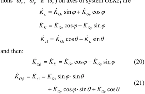
Motion of the Solar system bodies is considered in non-rotating barycentric ecliptic coordinates x10y10z10
(Figure2) connected to the Earth’s orbital plane fixed at T0 epoch. Axis x10 is pointed toward the vernal equinox.
Let the non-rotating system of geocentric ecliptic coor- dinates x1y1z1 with the center of mass at O moves transla-
tionally relative to the system x10y10z10. Axis z of the ro-
tating geocentric ecliptic coordinates xyz is directed along the Earth’s own angular velocity and axis x at the initial moment t = 0 lies in the Greenwich Meridian plane. The Earth’s absolute angular velocity in sys- tem x1y1z1 with the projections ωx,ωy,ωzto rotating axes
of system xyz will be
φ
ω
ω ix jy kz.
In the law (1), angular momentum KO is produced by all the masses of rotating Earth in system x1y1z1, and
mO Fk is moment of forces produced by all the Solar system bodies. First define derivation of the angu- lar moment and then the sum of torques.As in system x1y1z1 the Earth rotates with angular ve-
locity , thus any of its element dM with a radius vec- tor
ω
j k
r ix y z (Figure 2) moves with velocity
r
ν ω and has angular momentum
mO dMν r vdM relative to the center O.
After integration taking into account the entire Earth’s mass M, KO is
O O
M M
dM dM
v
r vK m (6)
Having differentiated KO
ω ν
on time and then having substituted vectors , and , after transformation we obtain derivatives of the projections of the angular momentum to axes of rotating system xyz
r
2 2
y z x xz z
y z yz y z
J
J
Ox x x xy y x
y z
J J
J J
K
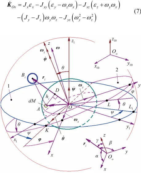
[image:4.595.309.538.338.622.2](7)
2 2
Oy y y yz z x y yx x z y
z x z x zx z x
J J J
J J J
K (8)
2 2
Oz z z zx x y z zy y x z
x y x y yx x y
J J J
J J J
K (9)where εx,εy,εzare projections of the Earth angular accel- eration in system x1y1z1 to axes of rotating system xyz;
2 2
d
xM
J y z M,
2 2
d
y M
J z x M ,
2 2
d
zM
J x y M
xy M
—the Earth’s axial moments of in- ertia, and J xy Md , xz
d ,M
J xz M
d
yz M
J yz M —its centrifugal moments of inertia. As the system xyz is connected with the rotating Earth, the moments of inertia do not depend on the Earth’s rota- tion and remain constants. Today’s knowledge of the Earth’s density distribution is insufficient for definition of the moments of inertia. As it will be shown below, it is possible to define only the relation between two mo- ments of inertia Jz and Jx, from observable angular veloc- ity (precession), but not their absolute values. Last years the three-axial model of Earth is described where the third moment of inertia is estimated by potential of the gravitational distribution on Earth’s surface. How- ever, this method can not give precise estimation of the moments of inertia. Note, that in case of three-axial Earth it is required to add terms with centrifugal moments of inertia because of nonsymmetrical distribution of poten- tial as shown from (7)-(9). Traditionally, terms with these moments are unaccounted and terms containing third moment Jy are in equations though in last forms Jy is equal Jx. Nevertheless, avoiding of complications with unaccounted terms it is considered axisymmetrical Earth Jy= Jx,and Jxy= Jxz =Jyz= 0. Then derivatives of the angular momentum (7)-(9) are:
ψ
, , .Ox x x y z y z
Oy y y z x z x
Oz z z
J J J
J J J
J K K K (10)
For axes with zero centrifugal moments of inertia the moments Jx, Jy, Jzare named principal moments of iner- tia.
3.2. The Law of Angular Momentum in Euler Angles
Position of rotating system xyz (Figure 2) relative to
non-rotating system x1y1z1 is determined by Euler angles:
, , , here precession angle defines position of nodes line OK, where moving equatorial plane inter- sects fixed orbital plane (ecliptic), nutation angle defines a tilt between equatorial plane and ecliptic and
is angle of the Earth’s own rotation around axis z. Figure 2 shows directions of this angles accepted in theoretical mechanics. In astronomy angles, which are directed according to observably movements, are ac- cepted: a 2 , a and a . Directions of angular velocities are shown on Figure2, i.e. turn of angles
,
ψ θ, φ
, and is visible counter- clockwise from the side of these vectors. It is seen from Figure 2 that Euler’s velocities stay constant at the Earth’s turn. Therefore let all the variables and equations will be expressed in Euler variables.
As it is possible to present the vector of absolute an- gular velocity as (2), thus in projections to axes x, y, z it is
,
x x x x
y y yy,z z zz
(11) where x, x,
x
etc. —projections of the Euler an- gular velocities to axes xyz. Having calculated expres- sions (11) with the help of Figure2 it is received Euler well-known equations:
sin sin cos , sin cos sin ,
cos . x y z ψ θ ψ θ φ ψ
(12)
After differentiation (12) the angular accelerations in Euler variables become:
sin sin cos sin sin cos cos sin ,
x ψθ
ψφ θφ (13)
sin cos cos cos sin sin sin cos ,
y ψθ
ψφ θφ (14)
cos sin
z
ψθ (15)
Having substituted angular velocities (12) and angular accelerations (13)-(15) in (10), the projections of deriva- tives of the angular momentum depending on Euler an- gles are:
2
sin sin cos 2 cos sin
sin cos sin ( ) sin cos cos
Ox x x
x z z z z x J J J J J J
J J ;
K ψθ
2
sin cos sin 2 cos cos
sin sin cos ( ) sin cos sin ;
Oy y y
x z
z z
z x
J J
J J
J J
J J
K
θψ
ψφ θφ (17)
cos sin
Oz JzJz Jz
K ψθ (18)
Let us transform the law of the angular moments (1) to Euler angles. The moments of forces can be defined di- rectly through forces for the actions of each body on an Earth mass element (see Figure2). However, hereinafter at their series representation they are reduced to other terms. Here we define the moments through the force function U by a traditional method to safe continuity with previous works. As it is known from the theorem of theoretical mechanics, the moments of forces in a direc- tion of axes are equal derivatives of force function on an angle of turn relatively to this axis. Therefore in system OKz1z with the axes located on vectors of angular veloci-
ties ψ, θ and , the moments of forces are (φ Figure 2): mO mOz1 U , mO mOK U ,
O Oz U
m m . Taking into account these mo-
ments we project the right and left part of (1) on the axes of system OKz1z:
O
K U , KO U , KOz U (19) Let us express derivatives of the angular momentum in Equation (19) through derivatives KOx, KOy and KOz in Cartesian coordinates Oxyz, and draw axis OL perpen- dicularly to axis OK (Figure2).
Then, projections of the derivatives KOx, KOy and Oz
K (on Figure2 are not seen but identical to project- tions x, y и z) on axes of system OLKz1 are
sin cos
L Ox Oy
K K K
cos sin
K Ox Oy
K K K
1 cos sin
z Oz L
K K K
and then:
cos sin
K Ox Oy
O
K K K K (20)
1 sin sin
cos sin cos
O z Ox
Oy Oz
K K K
K K
(21)
Further the Cartesian projections (16)-(18) are substi- tuted in Equations (20) and (21), and the last ones are substituted in (19) in system OKz1z. Then, having ex-
pressed the second derivatives it is received two differ- ential equations of the Earth’s spin in Euler’s variables:
2
2 sin cos sin
1
cos sin
x z z
Oz
x x
U J J J
K J J
ψθ θφ
(22)
2sin cos sin 1x z z
x
U J J J
J
(23) where the derivative of the angular momentum KOz is defined by the third formula in the equations (19) for the law of angular momentum.
3.3. The Force Function in Cartesian Coordinates
Now we define force function for the action of body Bi with mass Mi (Figure2) on the Earth by the traditional way presented, for example, in [15]. Its coordinates in rotating system xyz are xi, yi, zi. The force function of the action of this body on the Earth’s element of mass dM with coordinates x, y, z is i ,
di GM dM dU
r
where G is the gravitation constant,
2
2
di i i i
r x x y y z z 2
is the distance be- tween the element of mass dM and the body Bi. Having summarized on all Earth’s mass M and on all bodies n the force function is:
1
d
n
i
i M di
M
U GM
r
(24)where dM d d d ;x y z
x y z, ,
is the Earth’s density.It is obviously impossible to integrate Equation (24) because today’s distribution of the Earth’s density is studied only qualitatively. Therefore direct definition of the force function for the action of external bodies on the Earth as mechanical system is impossible. All further solutions are in simplification of Equation (24) and in derivation of the force function depending on the Earth’s moments of inertia Jx, Jy, Jz. Correlation between them are defined on observable rate of the Earth’s pre- cession.
[image:6.595.56.288.500.651.2]
22 2 1
di i i i i i
r r r r b (25)
where
2
2
2i i i i r r b r .
As bi 1, then subintegral function 1rdi in (24) is represented as Taylor series at b powers. Taking into account terms that are no more the fourth order in rela- tion to bi , the force function is in form
2 2 3 2
2 3
1
4 2 2 4
4
3 5 3
1 ]
2 2
35 30 3
d 8
n
i i i i i
i i M i i i
i i
i
GM r r
U
r r r r
r r M r
(26)Line segment i (Figure2) is expressed through co- ordinates x, y, z of the element dM by means of direction cosines i,i,i:
ˆ ˆ ˆ
i l x m y n zi i i
(27) where
ˆ cos ,
ˆ cos ,
ˆ cos .
i i i i
i i i
i i i i
l x m y n z i r r r (28)
By definition, the axes of a body, which are on inter-section of planes of symmetry, are the principal axes of inertia. Axes of rotating system Oxyz are directed along the Earth’s principal axes of inertia. Therefore integrals of type k
, , d ,
M
x f x y z M
where k—an odd integer,and f x y z
, ,
x
—even function of coordinates, will con- sist of two equal on size and opposite on a sign parts at the intervals and , i.e. these integrals are equal zero in the sum. Because, according to (27), vari- able i
0
x0
is proportional to coordinates x, y, z, the inte- grals in (26), depending on and 3, are equal zero.
Note, that these integrals are necessary to consider in case of the non-symmetrical Earth and absence of sym- metry on one of the planes zOx or zOy, i.e. the force function as well as the derivatives of angular momentum (7)-(9) will include centrifugal moments of inertia.
Integral of the first term in (26) is the Earth’s mass. Numerator of the third term with the account (27) is
2 2 2 2 2 2 2 2 2 2 2
2 2 2
ˆ ˆ ˆ ˆ
3 3
ˆˆ ˆˆ ˆ ˆ 2
i i i i i
i i i i i i
r x m x n x m y n z
x y z l m xy l n xz n m yz
(29) As thus in (29) it is taken into, that . The terms integration having co-
2 2 2
ˆ ˆ ˆ 1,
i i i
l m n
2 1 ˆ2 ˆ2
i i i
lˆ m n
ordinates in the second power gives the moments of iner- tia and the last ones gives centrifugal moments as
d xy
J
xy M which are zero for the Earth with prince- pal axes along x, y, z.After substitution (29) in (26) and integration we ob- tain the force function without the last fifth term
1
2 2
3
ˆ ˆ
2 3 3
.
2 n
i i
y z x x y z x
i i
U GM
J J J m J J n J J
M r r
(30) In this case the action on the Earth’s rotational motion is defined by the third and the fifth terms in (26) as they depend on Euler angles. Having divided the fifth term on the third, we find that the order of their relation is equal2 2
E i
R r where RE—radius of the Earth. This ratio has the greatest value for the Moon, and is equal 310–4. Further
the bodies’ action on the Earth’s spin is considered with such relative error. Therefore additional effects should be considered, if the relative value of their action has the order 310–4 and more.
After the direction cosines and are substituted according to (28), force function (30) becomes
ˆ
m nˆ
1 2 2 3 5 2 . 3 2 2 n i ix y i z x i
y z x
i i i
U GM
J J y J J z
J J J
M
r r r
(31) where yi and zi—coordinates of the body Mi in rotating system xyz.3.4. The Moments of Forces in Euler Angles We express yi and zi through coordinates x1iy1iz1i of sys- tem x1y1z1 (Figure 2). Let us draw the line OL1 perpen-
dicularly to OK in the plane x1Oy1. Coordinates of the
body Bi will give projection OL1i x1isin y1icos on this line and then coordinate z of the body Bi is
1 1
1 1 1
cos sin
sin sin sin cos cos
i i i
i i
z z OL
x y zi
(32)
Having defining projections of the coordinates x1i and y1i to the axes OK and OL analogously, coordinate yi is
1
1
1
Earlier we neglected the centrifugal moments of iner- tia. It is admissible, if the Earth is axisymmetrical, or axes x and y lie in symmetry planes. As there is no evi- dence on presence of such planes we should consider the axisymmetrical Earth with the equal moments of inertia relative to axes x and y, i.e.Jy=Jx. Therefore we do not present bulky expressions for the non-axisymmetrical Earth. If necessary they may be received on be- low-mentioned sequence with use of expression (33). For the axisymmetrical Earth, after substitution (32) in (31), taking into account Jy= Jx, force function becomes:
5 1
2
1 1 1
2 1
3 2
sin sin sin cos cos
2 n
i
z x
i i
i i i
n
i z x
i i i
GM
U J J
r
x y z
GM J J
M r r
(34)
After differentiation (34) on Euler angles φ,ψ,θ and reductions we obtain the moments of forces
0 Oz U
m (35)
1 5
1
2 2 2 2
1 1 1 1
1 1 1
3
sin sin cos sin cos 2
sin cos cos sin
n i
Oz z x
i i
i i i i
i i i
GM U
J J
r
x y x y
z x y
m (36)
5 12 2 2 2 2
1 1 1 1 1
1 1 1
3
sin 2 2
sin cos sin 2 2 cos 2 sin cos
n i
OK z x
i i
i i i i i
i i i
GM U
J J
r
x y z x y
z x y
m (37) 3.5. Differential EquationsThe law (1) in projection to the axis z of rotating system xyz, according to (19), has a form KOz U . We consider the rigid Earth during derivation of the equa- tions: Jz = const. The moment of inertia of the axisym- metrical Earth JOz may be changed for the action of re- distribution of a water cover, thawing of glaciers, mov- ing of continents, etc. In order to estimate the influence of these factors, it is entered Jz ≠ const. Therefore, ac- cording to (35) U 0, then and taking into account (10) at Jz = Jz0 it becomes
0 Oz K
z z
J 0. After integration it is JzzconstJz0z0, that may be
written in form
0 0
z z Jz Jz
(38) where Jz0and ωz0 are the Earth moment of inertia and its
projection of angular velocity in an initial epoch. Be- cause zφ ψ+cos (according to Equation (12)),
thus, taking into account (38), we obtain angular velocity of the Earth’s own spin
0 0 cos
z Jz Jz
φ ψ (39) From expression (39) follows that angular velocity of the Earth’s own spin , which is not connected with motion of vector of angular speed , may be changed via redistribution of the Earth’s moment of inertia and alteration of precession rate. Expression (39) for angular velocity of the Earth’s own spin may be used for an es- timation of the Earth’s parts motion influence on its an- gular speed.
φ
ω
Having designated a projection of the Earth’s angular velocity zz0E const
0
Oz Oz
, expression (39) for the rigid Earth J J const we rewrite in a kind
cos
E
φ ψ (40) After substitution of , and the derivatives of the force function (36) and (37) in Equations (22) and (23), differential equations of the Earth’s rotational movement are
φ KOz 0
2 2 1 1 5 11 1 1 1 1
cos 2 sin sin 3 0.5sin 2 cos
cos 2 cos sin sin
z E x n
i d z
i i
i i x
i i i i i
J J GM E J
x y
r J
x y z x y
ψθ
(41)
2 2 2 1 5 12 2 2
1 1 1 1
1 1 1
sin 0.5 sin 2
3
sin 2 sin 2
cos sin 2 2 sin cos cos 2
z E x n
i d z
i
i i x
i i i i
i i i
J J GM E J
x r J
y z x y
z x y
ψ
(42)
where d
z x
z is the Earth’s dynamical el- lipticity;E J J J
E
projection of the Earth’s absolute angular velocity to its axis z, and ratio of moments is
1 1
Jz Jx Ed .
As E = const and changes according to (40), thus value
φ E
may be obtained as a result of averaging of the measured values φ иψcos on time, i.e.
cos
φ ψ . E
4. Initial Conditions and the Earth’s
Dynamical Ellipticity
We study the action of separate bodies on the Earth, therefore at integration Equations (41) and (42) it is nec- essary to set initial values for alteration of rates and
, which are determined by influence of each body. At any set of initial values ψ and there begins a tran- sient response, which may become whether a steady- state regime in a long time or not to be steady state at all. We are interested in the Earth’s behavior at steady-state regime. Let the second derivatives and in Equa- tions (41) and (42) are small in relation to the other terms at steady-state regime, i.e. 0. As
E
exceeds the derivatives ψ and on 6 orders therefore at ne- glecting terms with ψθ and 2 in Equations (41)and (42) they become
5 1
2 2
1 1 1 1
1 1 1
3 sin 2
sin 2 2 cos 2 cos
2 cos sin sin
n
i d
i E i
i i i i
i i i
GM E r
x y x y
z x y
(43)
5 12 2 2 2 2
1 1 1 1
1
1 1 1
3
sin 2 2 sin
sin cos sin 2 2 sin cos cos 2
n
i d
i E i
i i i i
i i i
GM E r
xi y z x y
z x y
(44)
Equations (43) and (44) are identical to the Poisson equations; their approximate solutions are applied in as- tronomical theories of climate change. We will define initial values of derivatives from these equations, setting coordinates x1i, y1iand z1i of bodies acting on the Earth during an initial epoch t = 0. Initial values of the angles are: 00 and 00, where 0 = 0.4093197563 is the inclination due to an initial epoch, for example 30.12.1949.
There is the unknown parameter d
z x
z , which defines relation between the Earth’s moments of inertia. Today’s knowledge of the Earth’s density distri- bution is insufficient for definition of the moments Jzand Jx with a demanded accuracy. Therefore the Earth’s dy- namical ellipticity Ed is defined by comparison of the calculated precession rate with the observations. Ac- cording to [16,17] the Earth’s precession has clockwise direction relative to the fixed ecliptic and during a tropi- cal year isE J J J
1 50".37084 0".00493
p T (45) where T is counted in tropical centuries from a funda-
mental epoch 1900.0 with JD = 2415020.3134. In an initial epoch it is p1050".3733046" yr. Observable
average precession rate is described by Equation (45). Now we define its calculated value according to (44). If an initial epoch coincides with an epoch of reference frame, then 0 and 0. Then Equation (44) is
written
2 2
0 3 0
1
1 1 0 0
3
cos
cos 2 sin
n i
d i
i E i
i i GM E y r z y
1 z1i
(46)
where x1ix r1i i, y1i y r1i i,
1i 1i
z z ri —dimensionless coordinates of acting bodies. If a reference epoch does not coincide with an epoch of reference frame, 0, and 0.
In the course of cyclic relative movement of bodies round the Earth all coordinates change similarly, for example x1 maxi x1ix1 maxi . Hereat x1 maxi y1 maxi 1, and z1 maxi sinii, where ii—the tilt between the body’s orbital plane and equatorial plane. Since Pluto has the most value of the tilt ii = 0.7 [6], for all planets z1 maxi 1. The second term in a square bracket (46) will change in limits sin cos 2ii
0 sin0 and averaging on timewill make it zero. The maximum value of the factor of the first term
2 2
1i 1i
y z is 1, and minimum is zero, therefore and av-
eraging on time will give 0.5. Then all the part in square brackets at averaging is 0.5cos0.
Value of geocentric distances to the planets changes in limits RpiRpE ri RaiRaE, where Rpi, pE and
ai, aE – perihelions and afelions of the planets and the Earth, accordingly. Then average geocentric distance to the planets is
R
R R
0.5im ai aE pi pE
r R R R R (47) which is rim
RaiRaE RpiRpE
0.5 for internal planets, and aia eE E for external, where ai, aE and ei, eE—semimajor axes of heliocentric orbits and orbits ec- centricity of the planets and the Earth accordingly. Ac- cordingly, for the Sun and the Moon average geocentric distances areSm E
r a , rMmaM (48) where aM—average semiaxis of the Moon’s orbit. Then average value of speed of precession, according to (46), one gets 0 0 3 1 1.5 cos n i m d
i E im
GM E r
(49)
average precession rate and observed one
0m p10 Yr rdtr
, where 365.25636042 24 3600 tr
Yr —duration of a sidereal
year in sec, and rd180 360 0 we find the dynami- cal ellipticity
0
10 3
1
1.5 cos
n
i
da tr
i E im
GM
E p Yr rd
r
(50)
where index a and Eda denote approximate method of calculation of this value.
Having derivated Equations (49) and (50) we averaged enough approximately expression (46) on time, for ex- ample, the average values and ri can essentially dif- fer. If laws of planets motion x1i(t), y1i(t), z1i(t) could be found, there were known average value 0
3
i r
on time span T by integrating expression (46) on time at interval from 0 to T. However, expression (46) is approximate since it is obtained from the equations of motion at ne- glecting and . Therefore Equation (50) repre- sents the Earth’s dynamical ellipticity approximately. Its more exact value will be obtained after numerical solu- tion of the Earth’s rotational movement Equation (41) and (42) and comparisons of averaged from short-period oscillations of dynamics during known observation with observable dynamics of average precession for this period.
ψ
The value of dynamical calculated according to (50) under the data used by us, is Ed0 = 3.324257·10–3. Tradi-
tionally dynamical ellipticity is calculated with the ac- count only the Moon and the Sun. In this case, under our data EdSM1 = 3.324268·10–3i.e. differs at unit of the sixth
positional notation. As it is seen from (50), the dynami- cal ellipticity depends on averaged distance , thus the small changes of its value sufficiently change Eda.
3
im r
For instance value of this distance for the Moon
8
3.838 10
im M
r a м, which we obtained at reference conditions at epoch 30.12.49 from ephemerides DE406, gives dynamical ellipticity EdSM2 = 3.324770·10–3. To
comparison here are ellipticities used by various authors: Bretagnon and Simon [11] EdB = 3.2737671·10–3; F. Roosbeek and V. Dehant [18] Ed = 3.273767·10–3; Laskar et al. [5] Ed = 3.28005·10–3 with using aM = 384747980 м and p10 = 50.290966''/yr.
As we see, values Ed in expression (50) change de- pending on the accepted data in the second significant figure. The value dynamical ellipticity, taking into ac- count the data accepted by us, is designated as Ed0, and
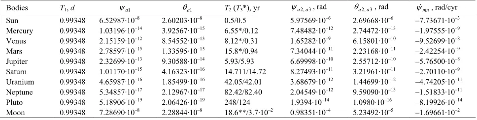
according to Simon et al. [19] as EdS. Table 1 gives Earth’s axis mean precession rates for the action of the Sun, the Moon and the planets calculated according to (49) and Ed= EdS. The most value of speed of precession is caused by the Moon, the action of the Sun is twice less, and Venus and Jupiter cause the greatest action from the
planets. As it is seen from Table1, difference between speed of precession 0m for the action of all the bod- ies and observable value p10 is 3.14·10–3%.
Due to accepted dynamical ellipticity EdS and 0 0,
0 0
, initial values 0 and 0 are calculated ac-
cording to (43) and (44) for the action of the separate bodies and all together, see Table1. Note, that expres- sions (43) and (44) represent values of derivatives 0
and 0 approximately. Their exact value is given by
observation. There are no these values for the action of separate bodies but there are observation data for the simultaneous action of all the bodies on the Earth. How-ever, as Equations (43) and (44) are approximate, total values 0 и0 (taking into account all the bodies) will
differ from the observation data.
5. Solution Algorithm
The coordinates x1i, y1i, z1iof the bodies Mi, acting the Earth in Equations (41) and (42) are referred to the fixed geocentric ecliptic coordinates (Figure 2). Numerical solution of the orbital problem gives the change of their orbit parameters i,φΩ,φp, Rp, e over a time span 100 Myr [6]. Due to this solution there are the bodies’ positions saved with 10 kyr interval. To integrate equations of ro- tational motion one needs the bodies’ positions during any moment of time.
[image:10.595.309.537.557.721.2]The bodies’ positions are usually set on the base of the theory of secular perturbations during solving rotational motion equations. Bretagnon et al. [11] used epheme- rides DE403 for numerical integration of these equations for 1968-2023 yr interval. These methods are not suitable Table 1. The mean precession rate 0m of the Earth’s axis
and the initial rates 0and 0 for the separate action of
the bodies by results of computations according to (49) and (43)-(44), accordingly. Computations executed at EdS = 3.2737752·10–3; p
10 = 2.4422·10–2 rad/cyr; 00; 00;
rad in radians and cyr in centuries years.
0m
0 0
No. Bodies
rad/cyr
1 Sun –7.73095·10–3 –1.20483·10–6 –7.09773·10–8
2 Mercury –1.02693·10–9 1.42035·10–10 2.95503·10–11
3 Venus –1.86489·10–8 –7.17466·10–9 –2.99417·10–9
4 Mars –6.82598·10–10 –8.87394·10–12 1.26014·10–10
5 Jupiter –5.19060·10–8 1.58365·10–9 4.60379·10–10
6 Saturn –2.53056·10–9 1.06473·10–10 2.27373·10–10
7 Uranium –4.74989·10–11 1.45508·10–12 2.78046·10–14
8 Neptune –1.46677·10–11 –6.38274·10–13 8.18066·10–13
9 Pluto –6.92755·10–14 4.37046·10–13 1.91721·10–14
10 Moon –0.01657 –1.83206·10–3 –9.29602·10–4
for long-time integration. Therefore we developed the follow algorithm to compute the motion laws of the bod- ies x1i(t), y1i(t), z1i(t). Their coordinates are defined on the base of our solutions about motion of the Solar system bodies in fixed barycentric equatorial coordinates. Using orbital parameters i,φΩ,φp, Rp, e Cartesian coordinates are recalculated in polar ri and φi in orbital plane. To estimate the body position during new moment of time t1
= t+Δt one may use expressions for elliptical motion given in [12,13,20,21]: t = t(r)—motion law in implicit form and r(φ) – trajectory equation. Polar radius of the body r1 during new moment of time t1 is predicted under
Taylor’s formula of the second order, checked on de- pendence t1(r1) and then discrepancy for some iterations
comes almost to zero. After that from the trajectory equation there obtained polar angle φ1(r1) in a return
form. At small ellipticities e - 0 during new moment of time t1 under Taylor’s formula the angle φ1 is predicted,
checked under the movement law t1(r(φ1)), then the dis-
crepancy for some iterations also practically comes to zero.
This algorithm differs from the traditional. The inter- mediate parameters: mean anomaly M and eccentric anomaly E, which feature in traditional description of body motion on an elliptic orbit, are not used here.
The bodies polar coordinates r1,φ1 during any moment
of time are recalculated in coordinates of translationally moving geocentric system x1y1z1 via orbital parameters i,
φΩ,φp, Rp,. Since the orbital parameters change from one epoch to another, they are interpolated on a parabola on each step. Thus, the algorithm, which allows defining the bodies coordinates xi, yi, ziacting the Earth at any mo-ment from the considered interval of time, is developed. Note, that the Moon’s orbit has more short oscillation periods comparably with the other orbits of planets. Therefore the algorithm for the Moon was modified upon with their account.
We applied the Runge-Kutta integration of Equations (41) and (42). These algorithms of calculation of coordi- nates and numerical integration are programmed on the FORTRAN. The computation was run on personal com-puters and supercomcom-puters MVS-1000 at Keldysh Insti-tute of Applied Mathematics of the Russian Academy of Sciences (Moscow) and NKS-30T at Siberian Branch of the RAS Computing Center (Novosibirsk). As a result of numerical experiments we accepted the initial integration step t = 110–4 yr.
6. Numerical Integration Results
6.1. The Sun’s Action
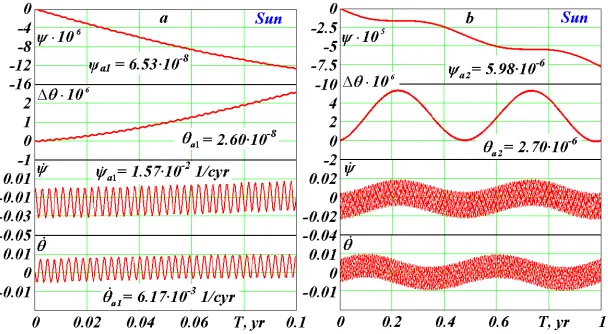
Figure 3, a gives results of integration Equations. (41)
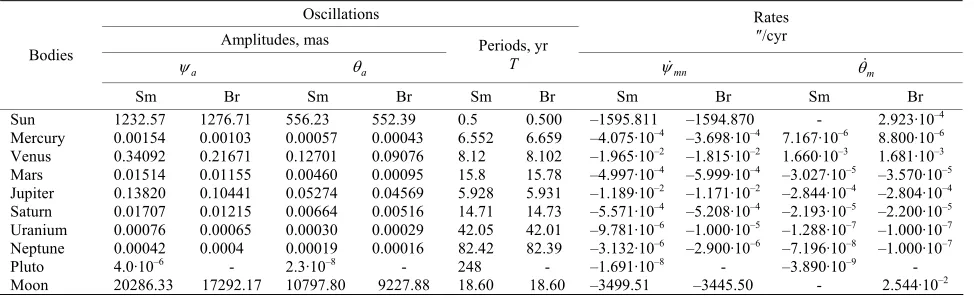
and (42) over 0.1 yr for the action of the Sun on the Earth’s rotational motion. The precession angle de- creases since zero value making fluctuations with the amplitude a1 = 6.53·10–8 rad = 13.47 mas and the pe-
riod T1 = 0.99348 d, where: mas is 10–3 angular seconds,
d is duration of a day in sec. The nutation angle is pre- sented as difference 0, where θ0= 0.4931976 rad. As it is seen from the graph value of the tilt between moving equatorial plane and fixed ecliptic increases, making fluctuations with amplitude a1
T
= 2.60·10–8 rad = 5.27 mas and same period T
1. Rate of
precession
oscillates round some mean value with period T1 and amplitude a1 = 1.57·10–2 rad/cyr. Rateof nutation oscillates with the same period T1 and ampli-
tude a1 = 6.17·10–3 rad/cyr round almost zero value.
As it is seen from Figure3, a initial values of the rates
0
and
0
do not exceed their extreme values. There- fore an error in definition 0 and 0 causes only
change of an initial phase of fluctuations. Hence, in this case dynamics of the rates 0 and 0 is not changed
at an error of initial conditions described in p. 4. There are similar properties of solutions for the action of other bodies, thus this property will be kept for the action of all bodies. Consequently, the initial conditions in this case calculated according to (43), (44), may be specified on a phase of observed daily oscillations and .
As the accepted initial conditions, according to (43), (44), are artificial, there arises the question. Which val-ues of derivatives 0and 0 might be, if a long-time
action of a single body on the Earth preceded the begin- -ning of calculation? Apparently, there would be an oc- currence of equilibrium and derivatives would come nearer to the mean values. With this purpose there were defined mean values 01 = 1.61891·10–2 and 01 =
–1.32398·10–3 according to the first daily oscillations
(see Figure 3(a)). Integrating Equations (41)-(42) with initial values 01
and 01 has resulted in reduction of
daily oscillations in 20 times (see Table2). Hereat char- acter of solutions behavior for the long-time actions has not changed.
At averaging derivatives in new solutions there ob- tained mean values 02 = 1.59342·10–2 and 02 =
–1.08328·10–3, submitted in Table 2. Repeated calcula-
tion with these initial values has resulted in diminution of amplitudes of oscillations in several times. Thus, there were executed 4 calculations with specification of the mean values of initial rates. Consequently, amplitudes of daily oscillations have decreased in several hundred times, according to Table2.
It is possible to account the final values of derivatives
0
and 0 as steady-state for long-time action of a
Figure 3. Action of the Sun on the Earth’s rotation: a – during 0.1 yr; b – during 1 yr. Precession angle and nutation an- gles difference 0 are in radians and rates and are in radians per century; T—begins with initial epoch
[image:12.595.57.287.329.416.2]30.12.1949.
Table 2. Amplitudes of daily oscillations for the action of the Sun at specification of the steady-state initial rates.
Initial rates Daily amplitudes
0
0
a
a
No.
rad/cyr
1 –1.20483·10–6 –7.09773·10–8 1.55690·10–2 6.17065·10–3
2 –1.61891·10–2 1.32398·10–3 8.53536·10–4 3.72235·10–4
3 –1.59342·10–2 1.08328·10–3 2.38888·10–4 1.39865·10–4
4 –1.59710·10–2 9.90860·10–4 2.48460·10–5 5.10429·10–5
several bodies there, apparently, will not be such steady-state condition for each body. Therefore further we consider the action of single bodies at initial condi-tions, according to (43), (44).
Figure 3(b) shows the Earth’s axis dynamics for 1 yr. The precession angle increases clockwise making oscil- lations with period T2 = 0.5 yr and amplitude a2=
5.98·10–6рад = 1232 mas. The nutation angle oscillates
with the same period T2 and amplitude a2 = 2.70·10–6
рад = 556.9 mas around mean value. A minimum of the Earth’s inclination is in the reference epoch (30.12.1949). It is explained by the most deviation of the Sun from the equatorial plane, which makes the most moment of force giving min.
Figure 4(a) presents axis dynamics for 10 yr. The precession angle changes practically linearly with semi-annual oscillations marked earlier, and the nutation angle with the period T2 oscillates about mean value. The
rates and with the periods T1иT2 change in the
same bounds, as on Figure 3(b). The Earth’s axis dy- namics over 100 yr is shown on Figure4(b). The pre- cession angle changes linearly with mean rate
mn
= 7.74·10–3 rad/cyr during 1000 yr. The nutation
angle in the form of changes with daily and
semi-annual periods in invariable limits. The rates and oscillates also in invariable bounds: around the mean value mn, and around almost zero value. The parameters behavior over 1000 yr is the same, therefore these results are not submitted here.
Obtained as a result of integration (41), (42) the mean value of precession rate coincides with the mean value
0m
= 7.73·10–3 rad/cyr calculated on the approximate
dependence (49), (Table1). It is necessary to notice that the instant precession rate (Figure 3(b)) changes in bounds minψ max, where max= 0.016 rad/cyr,
and min
0
= –0.032 rad/cyr, i.e. changes more than in 20 times relative to an average. The rate changes in more relative bounds in relation to its mean value
m
ψ
θ
. However, at such considerable changes of the instant rates и the mean values remain constants during all integration interval. It testifies stability of the integration method. And as mean values mn
ψ θ
corre- spond with observations, it testifies reliability of the so- lution of the entire problem.
Note, that under consideration of the action of the body B on the Earth (Figure1) there was shown that the torque m0 < 0and the precession rate < 0. As a result of integration (41), (42) we have received that precession rate takes positive values also (Figure3(b)). This result is caused by dynamics: under the action of torque the Earth’s axis speeds up, according to (4), and its motion proceeds even in absence m0 due to inertia. Therefore
ψ
min max
is more than the value given by (4), and > 0. Here we do not submit graphs of the Earth’s angular velocity dynamics , since, according to (40), the hanges of have contrary sign to the changes of the precession rate . This conclusion is proved by results of other authors, for example, [9].
φ