Unsteady Boundary Layer Flow past a Stretching Plate and
Heat Transfer with Variable Thermal Conductivity
Mamta Misra1, Naseem Ahmad2, Zakawat Ullah Siddiqui3 1Depatment of Applied Sciences, NSIT, New Delhi, India 2Department of Mathematics, Jamia Millia Islamia, New Delhi, India
3Department of Mathematics & Statistics, Faculty of Science, University of Maiduguri, Maiduguri, Nigeria
Email: mamtansit@yahoo.co.in
Received November 10,2011; revised December 15, 2011; accepted December 25, 2011
ABSTRACT
An unsteady boundary layer flow of viscous incompressible fluid over a stretching plate has been considered to solve heat flow problem with variable thermal conductivity. First, using similarity transformation, the velocity components have been obtained, and then the heat flow problem has been attempted in the following two ways: 1) prescribed stretching surface temperature (PST), and 2) prescribed stretching surface heat flux (PHF) Flow and temperature fields have been analyzed through graphs. The expressions for skin friction and coefficient of convective heat transfer Nusselt number in PST and PHF cases have been derived.
Keywords: Unsteady Boundary Layer Flow; Skin Friction Energy Equation; Nusselt Number
1. Introduction
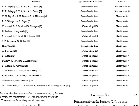
Due to number of applications in industrial manufactur-ing process, the problem of boundary layer flow past a stretching plate has attracted considerable attention of researchers during the past few decades. Examples of such technological process are hot rolling, wire drawing, glass-fiber and paper production. In the process of draw-ing artificial fibers the polymer solution emerges from orifice with a speed which increases from almost zero at the orifice up to a plateau value at which remains con-stant. The moving fiber, which is of great technical im-portance, is governed by the rate at which the fiber is cooled and this, in turn affects the final properties of the yarn. A number of works are presently available that follow the pioneering classical work of Sakiadis [1], F. K. Tsou, E. M. Sparrow, R. J. Goldstein [2] and Crane [3]. Table 1 lists some relevant works that pertain to cooling liquids, i.e., heat transfer for stretching surface.
There are liquid metals whose thermal conductivity varies with temperature in an approximately linear man-ner in the range from 0˚F to 400˚F. In 1996, T. C. Chiam [21] considered heat transfer problem with variable ther-mal conductivity in stagnation-point flow towards stret- ching sheet. Naseem Ahmad and Kavita Marwah [22] also studied boundary layer flow of Walters Liquid B Model with heat transfer for linear stretching plate with variable conductivity numerically. In 2010, Ahmad and Mishra investigated unsteady boundary layer flow and heat transfer over a stretching sheet [23].
In almost all the problems of stretching sheet with heat transfer where closed form solution is obtained, the thermal conductivity of liquid has been taken constant. The present paper is the extension of the work done by N. Ahmad and M. Mishra [23] assuming that the thermal conductivity varies in linear manner with temperature. The temperature field has two parts: one mean tempera-ture, other is due to variable thermal conductivity. Both the parts mean temperature and temperature due to vari-able thermal conductivity have been analyzed thoroughly for some new recommendations.
2. Mathematical Formation and Solution
The problem considered here is the unsteady boundary layer flow due to a stretching flat plate in a quiescent viscous incompressible fluid. The flow is two dimen-sional where x-axis is along the plane of moving plate and y-axis is normal to it, respectively. We assume that the surface is moving continuously with the velocity; , 1
s
bx
u a b R
at
and t < 1/a in the positive x-direc-
tion. Under these assumptions, the boundary layer flow along moving plate is governed by the equations
0 u u x y
(2.1)
2 2 v
u u u
u
t x y
u x
Table 1. Some relevant works that pertain to cooling liquids.
Author/s Type of visco-elastic fluid Remarks
K. R. Rajagopal, T. Y. Na, A. S. Gupta [4] Second order fluid Not heat transfer
K. R. Rajagopal, T. Y. Na, A. S. Gupta [5] Second order fluid Not heat transfer
N. M. Bujurke, S. N. Biradar, P. S. Hiremath [6] Second order fluid Heat transfer
B. S. Dhanpat, A. S. Gupta [7] Second order fluid Heat transfer
N. Ahmad, G. S. Patel and B. Siddappa [8] Walter’s liquid B Heat transfer
D. Rollins, K. Vajravelu [9] Second order fluid Heat transfer
N. Ahmad, G. S. Patel, B. Siddappa [10] Walter’s liquid B Heat transfer
S. P. Lawrence, N. B. Roa [11] Second order fluid Heat transfer
M. I. Char [12] Second order fluid Heat transfer
A. Naseem [13] Walter’s liquid B Heat transfer
N. Ahmad [14] Walter’s liquid B Heat transfer
D.Kelly, K. Vjravelu, L. Andrews [15] Walters’ liquid B Heat transfer
N. Ahmad, K. Marwah [16] Walter’s liquid B Heat transfer
A. M. subhas, A. Joshi, R. M. Sonth [17] Walter’s liquid B Heat transfer
R. M. Sonth, S. K. Khan, A. M. Subhas [18] Walter’s liquid B Heat transfer
Siddheshwar, Mahabaleswar [19] Walter’s liquid B Heat transfer
M. Subhas Abel, P. G. Siddheshwar, Mahantesh M. Nandeppanavar [20] Walter’s liquid B Heat transfer
where u, the horizontal velocity component; v, the verti-cal velocity component; , the kinematic viscosity
The relevant boundary conditions are: y = 0, u = us, v = 0
y→, u = 0
Introducing the dimensionless variables
2
; ; ; ;
x y uh vh tv
h
x y u v t
h h v v
the Equations (2.1) and (2.2) reduce to
0 u u x y
(2.3)
2 2
u u u
t x y y
u (2.4)
with boundary conditions
0, , 0
, 0
s
y u u v
y u
(2.5)
where bar has been dropped for convenience. Setting the similarity solution of the form
1
bx
u f y
1
b
v f
at
y (2.6)
Putting u and v in the Equation (2.4), we have
2
1
af y bf y bf y f y at f y (2.7)
and the relevant boundary conditions become 0, 1, 0
y f f (2.8)
,
y f0 (2.9)
Boundary conditions suggest that the velocity function f may be of the form f
y erywhere r is unknown to be determined. Thus
1
ry bv e
r at
and the Equation (2.7) gives 1
a b r
at
. Therefore, we
have the velocity components as follows:
exp
1 1
bx a b
u y
at at
and
1
1 exp 1b a
v y
at
at a b
b
(2.10)
at
3. Skin Friction
The wall shear stress at the stretching plate is given by
0 w y u y 1 1 w
bx a b
at at
Thus, the skin friction is
1 2 1 w f e s a b C R at U h
(3.1)
4. Heat Transfer Problem
In absence of viscous dissipation and heat generation, the energy equation for two dimensional heat flow is given b
p
T T T
C u v k
x y y y
T (4.1)
subject to boundary conditions 0,
,
P
y T T
y T
(4.2)
where TP is plate temperature, T is temperature of
sur-rounding fluid, CP is specific heat at constant pressure
and k is thermal conductivity.
4.1. Case A: Prescribed Power Law Surface Temperature (PST)
Let the surface temperature be of the form 2 0, p
x
y T T T A
l
P T T T T while the temperature outside the dynamic region be . Now, we define the dimensionless tem-perature by
,
y TT ry
For liquid metals, it has been found that the thermal conductivity varies with temperature in an approximately linear manner in the range from 0˚F to 400˚F. Therefore,
we assume k as kk
1
where kp k k
. Now,
substituting u and v in the Equation (4.1) and changing the independent variable y to ry, we have
1 n
1
2
r a b e
p b
(4.3)
with boundary conditions
0, 1, , 0
(4.4)
The Equation (4.3) can be rewritten as
2
1
0
r
P b e
a b
(4.5)
From Equation (4.5), we note that the heat transfer takes place in two parts according to 0 and 0. If 0, then we have the main heat transfer due to con-stant thermal conductivity i.e.
1
0
r m
m
p b e
a b
(4.6)
0 1, 0 asm m
(4.7) and if 0, then we get the first correction equation to main heat transfer as
2 0
c c c
(4.8)
0 1, 0c c
, as (4.9) The solution of the Equation (4.6) is
0 1 d d , 1 , r r r b P e a b m b P e a b at P a b r r r r r e ea b b b
P P e
P at a b a b
b b
P P
a b a b
where
10
, t x d
x e t t
is incomplete gamma function
Equation (4.8) is a non linear differential equation of order two. Let the solution of this equation be of the form:
c
Putting this solution in Equation (4.8) we have 2
2 0 (4.10) The roots of this equation are 0 and 1/2. Therefore
1c
(4.11) The solution (4.11) of the Equation (4.8) does not sat-isfy the condition c 0 as . This condition is met only for 1. Therefore, the heat transfer in case
0
takes place within the dynamic region 0 1.
4.2. Nusselt Number
0 w y T q k y (*)
Therefore the Nusselt number is (see Table 2):
w
p
q Nu
k T T
0 1 exp1 1 1
, p y r r r k T Nu y
k T T
p at
a b a b
at at at
p p
a b a b
(4.12)
4.3. Case B: Prescribed Power Law Surface Heat Flux (PHF Case)
The power law heat flux on the surface of stretching plate is considered to be a quadratic power of x in the form 2 T x k D y l
at y0 (4.13) TT, as y (4.14)
where D is a constant, k is the thermal conductivity. Now we define dimensionless temperature g
by
, p T T g T T (4.15)
where 2 p D x T T kr l
when g
0 1where ry
Writing the Equation (4.2) in terms of g
, we getthe following differential equation
P br
1 e
2
0g g gg
a b
g (4.16)
together with boundary conditions: 1 at 0 0 as g g
[image:4.595.310.537.647.735.2] (4.17)
Table 2. Trend of Nusselt number.
t Nu for Pr = 1.54
Nu for
Pr = 2.15
Nu for
Pr = 5.10
Nu for
Pr = 9.42
0 0.2 0.4 0.6 0.8 1.0 26.356 19.976 15.332 11.828 9.212 7.271 95.389 64.026 43.062 29.255 20.043 13.906
4.574 × 10⁴ 1.667 × 10⁴ 6.012 × 10³ 2.234 × 10³ 834.364 312.276
0.343 × 10⁹ 0.522 × 10⁸ 0.795 × 10⁷ 116.283 × 10⁴ 185.922 × 10³ 28.727 × 10³
Equating the terms independent of and the terms in-volving from Equation (4.16), we get the following two boundary value problems:
r
1
0m
P b e
g g a b
m
(4.18)
and
2 0c c c
g g g (4.19)
where the nomenclature gm is main heat transfer when
thermal conductivity is constant and gc is correction to
the heat flow due to variation in thermal conductivity in PHF case. The solution of the Equation (4.18) together with the boundary conditions (4.18) is
r
da P
a b m
a
g e e
a b
(4.20)The general solution of the Equation (4.19) is
1c
g A B (4.21)
where we again observe that the dynamic region for this temperature field is 0 1. Hence, the boundary con-ditions (4.17) have been modified as
0c
g 1, and gc0 as 1 (4.22)
Using boundary conditions (4.22), the solution (4.19) becomes
2 1
v
g
4.4. Nusselt Number (See Table 3)
Recalling (*), we have
0 w y T q k y
02 r1
p y
P at
k T
Nu
y
k T T
1 a b a b e at
5. Discussion and Results
[image:4.595.59.286.648.736.2]The problem of unsteady boundary layer flow of viscous
Table 3. Trend of Nusselt number.
t Nu for Pr = 1.54
Nu for
Pr = 2.15
Nu for
Pr = 5.10
Nu for
Pr = 9.42
0 0.2 0.4 0.6 0.8 1.0 21.758 16.856 13.139 10.323 8.194 6.597 73.7 50.536 34.868 24.248 17.037 12.141
2.69 × 10⁴ 1.023 × 10⁴ 3.911 × 10³ 1.508 × 10³ 587.228 231.962
incompressible fluid overstretching plate has been ana-lyzed. The velocity field has been obtained by similarity transformation method. Later, the heat flow problem has been studied by considering PST and PHF cases. We summarize the results as in Figure 1 to Figure 6.
Figure1 shows that horizontal component of velocity
u. It increases as time progresses within the dynamical region [0, 1]. We also see that u is maximum in the im-mediate neighborhood of stretching plate and it starts decreasing as . In fully developed flow, as time goes on progressing, the velocity progresses too.
1
y
Figure 2 is a graph of v versus y for different instant of time. The vertical component v is almost constant within [0, 1] and later it starts increasing. v progresses as we march away from the slit and it also increases as time progresses.
Figure 3 is to study the variation of mean temperature field m with respect to Prandtl number Pr. We see that
as Pr increases, m decreases within dynamical region
[0,1] in PST case. As Pr ul v
decreases, i.e. kinematic
viscosity increases in turn viscosity of fluid increases. In case of more viscosity, generally flow of heat becomes slow. It is supported by our study.
Figure 4 is expressing the trend of temperature field
c
due to variable thermal conductivity. We see that the contribution of this temperature is more near the moving plate than as we go away from the plate in PST case. c
Figure 1. Velocity field at different instant of time.
Figure 2. Velocity component v at different instant of time.
Figure 3. Mean temperature field for different values of Prandtl number Pr in PST case.
Figure 4. Temperature distribution due to variation in ther-mal conductivity.
Figure 5. Skin friction with respect to time t.
is independent of Prandtl number Pr.
Figure 5 is the graph of ReCf versus time. We see that
as time progresses the skin friction increases .We mean that as time progresses the velocity increases, in turn skin friction increases.
Figure 6 is temperature field in PHF case. We see that it approaches to zero asymptotically.
We see the gm for Pr = 5.10 of liquid oxygen at 56˚K,
Pr = 2.15 of para-hydrogen at 14˚K and Pr = 1.54 of
liq-uid ammonia at 10˚C. It has been observed that gm
in-creases absolutely as Pr increases, but for Pr = 9.42 of
water at 10˚C, gm behaves in a different way due to its
density.
Nusselt number in PST case is given by the Equation (4.12) where we observe referring Table 2 that it de-pends on Prandtl number and time t as well. From Table 1 we find that as Prandtl number increases the Nusselt number also increases but Nusselt number decreases as time increases.
Referring Table 3 for PHF case, we see the same pat-tern as in PST case from Table 2.
We have not got Prandtl number from the temperature field due to variation in thermal conductivity.
REFERENCES
[1] B. C. Sakiadis, “Boundary Layer Behavior on Continuous Solid Surfaces: II Boundary Layer on a Continuous Flat Surface,” AIChE Journal, Vol. 7, No. 2, 1961, pp. 221-
225. doi:10.1002/aic.690070211
[2] F. K. Tsou, E. M. Sparrow and R. J. Goldstein, “Flow and Heat Transfer in the Boundary Layer on a Continuous Moving Surfaces,” International Journal of Heat and Mass Transfer, Vol. 10, No. 2, 1967, pp. 219-235. doi:10.1016/0017-9310(67)90100-7
[3] L. J. Crane, “Flow past a Stretching Plate,” Zeitschrift für Angewandte Mathematik und Physik, Vol. 21, No. 4,
1970, pp. 645-647. doi:10.1007/BF01587695
[4] K. R. Rajagopal, T. Y. Na and A. S. Gupta, “Flow of a Visco-Elastic Fluid over a Stretching Sheet,” Rheologica Acta, Vol. 23, No. 2, 1984, pp. 213-215.
doi:10.1007/BF01332078
[5] K. R. Rajagopal, T. Y. Na and A. S. Gupta, “A Non Simi-lar Boundary Layer on a Stretching Sheet in a Non-New- tonian Fluid with Uniform Free Stream,” Journal of Ma- thematical Physics, Vol. 21, No. 2, 1987, pp. 189-200. [6] N. M. Bujurke, S. N. Biradar and P. S. Hiremath,
“Sec-ond Order Fluid Flow Past a Stretching Sheet with Heat Transfer,” Zeitschrift für Angewandte Mathematik und Physik, Vol. 38, No. 4, 1987, pp. 890-892.
doi:10.1007/BF00946345
[7] B. S. Dhanpat and A. S. Gupta, “Flow and Heat Transfer in a Visco-Elastic Fluid over a Stretching Sheet,” Inter-national Journal of Non-Linear Mechanics, Vol. 24, No. 3, 1989, pp. 215-219. doi:10.1016/0020-7462(89)90040-1
[8] N. Ahmad, G. S. Patel and B. Siddappa, “Visco-Elastic
Boundary Layer Flow past a Stretching Plate and Heat Transfer,” Zeitschrift für Angewandte Mathematik und Physik, Vol. 41, No. 2, 1990, pp. 294-299.
doi:10.1007/BF00945114
[9] D. Rollins and K. Vajravelu, “Heat Transfer in a Second Order Fluid over a Continuous Stretching Surface,” Acta Mechanica, Vol. 89, No. 1-4, 1991, pp. 167-178. doi:10.1007/BF01171253
[10] B. Siddappa and M. S. Abel, “Visco-Elastic Boundary Layer Flow past a Stretching Plate with Suction and Heat Transfer,” Rheologica Acta, Vol. 25, No. 3, 1986, pp. 319-
320.
[11] S. P. Lawrence and N. B. Rao, “Heat Transfer in the Flow of a Visco Elastic Fluid over a Stretching Sheet,” Acta Mechanica, Vol. 93, No. 1-4, 1992, pp. 53-61.
doi:10.1007/BF01182572
[12] M. I. Char, “Heat and Mass Transfer in a Hydromagnetic Flow of Visco-Elastic Fluid over a Stretching Sheet,”
Journal of Mathematical Analysis and Applications, Vol.
186, No. 3, 1994, pp. 674-689.
doi:10.1006/jmaa.1994.1326
[13] A. Naseem, “On Temperature Distribution in a No-Parti- cipating Medium with Radiation Boundary Condition,”
International Journal of Heat and Technology, Vol. 14,
No. 1, 1995, pp. 19-28.
[14] N. Ahmad, “The Stretching Plate with Suction in Non- Participating Medium with Radiation Boundary Condi-tion,” International Journal of Heat and Technology, Vol. 14, No. 1, 1996, pp. 59-66.
[15] D. Kelly, K. Vjravelu and L. Andrews, “Analysis of Heat Mass Transfer of a Visco-Elastic, Electrically Conducting Fluid past a Continuous Stretching Sheet,” Nonlinear Analysis: Theory, Methods & Applications, Vol. 36, No. 6,
1999, pp. 767-784. doi:10.1016/S0362-546X(98)00128-X
[16] N. Ahmad and K. Marwah, “Visco Elastic Boundary Layer Flow past a Stretching Plate with Suction and Heat Transfer with Variable Conductivity,” International Jour- nal on Multicultural Societies, Vol. 7, 2000, pp. 54-56.
[17] A. M. Subhas, A. Joshi and R. M. Sonth, “Heat Transfer in MHD Visco-Elastic Fluid Flow over a Stretching Sur-face,” Zeitschrift für Angewandte Mathematik und Me- chanik, Vol. 81, No. 10, 2001, pp. 691-698.
doi:10.1002/1521-4001(200110)81:10<691::AID-ZAMM 691>3.0.CO;2-Z
[18] R. M. Sonth, S. K. Khan, A. M. Subhas and K. V. Prasad, “Heat and Mass Transfer in a Visco-Elastic Fluid Flow over an Accelerating Surface with Heat Source/Sink and Viscous Dissipation,” Heat and Mass Transfer, Vol. 38, No. 3, 2002, pp. 213-220. doi:10.1007/s002310100271
[19] P. G. Siddheshwar and U. S. Mahabaleswar, “Effects of Radiation and Heat Source on MHD Flow of Viscoelastic Liquid and Heat Transfer over Stretching Sheet,” Interna-tional Journal of Non-Linear Mechanics, Vol. 40, No. 6, 2005, pp. 807-821.
doi:10.1016/j.ijnonlinmec.2004.04.006
Dissi-pation and Non-Uniform Heat Source,” International Journal of Mass and Heat Transfer, Vol. 50, No. 5-6, 2007, pp. 960-966.
[21] T. C. Chiam, “Heat Transfer with Variable Conductivity in Stagnation—Point Flow towards a Stretching Sheet,”
International Communications in Heat and Mass Trans-fer, Vol. 23, No. 2, 1996, pp. 239-248.
doi:10.1016/0735-1933(96)00009-7
[22] N. Ahmad and K. Marwah, “Visco-Elastic Boundary Layer Flow past a Stretching Plate and Heat Transfer with Variable Conductivity,” Proceedings of 44th Congress ISTAM, 22-25 December 1999, pp. 60-68.
[23] N. Ahmad and M. Mishra, “Unsteady Boundary Layer Flow and Heat Transfer over a Stretching Sheet,” Pro-ceedings of 28th UIT Heat Transfer Congress, Brescia,