Computational Fluid Dynamics and Its Impact on Flow Measurements Using Phase Contrast MR Angiography

Computational Fluid Dynamics and Its Impact on Flow

Measurements Using Phase-Contrast MR-Angiography

Claus Kiefer*, Frauke Kellner-Weldon

Support Center for Advanced Neuroimaging, Institute of Diagnostic and Interventional Neuroradiology, University of Bern (Inselspital), Bern, Switzerland

Email: {*claus.kiefer, frauke.kellner-weldon}@csiro.au

Received December 14,2011; revised December 19, 2011; accepted January 6, 2012

ABSTRACT

Rationale and Objectives: Computational fluid dynamic (CFD) simulations are discussed with respect to their poten-tial for quality assurance of flow quantification using commercial software for the evaluation of magnetic resonance phase contrast angiography (PCA) data. Materials and Methods: Magnetic resonance phase contrast angiography data was evaluated with the Nova software. CFD simulations were performed on that part of the vessel system where the flow behavior was unexpected or non-reliable. The CFD simulations were performed with in-house written software. Results: The numerical CFD calculations demonstrated that under reasonable boundary conditions, defined by the PCA velocity values, the flow behavior within the critical parts of the vessel system can be correctly reproduced. Conclusion: CFD simulations are an important extension to commercial flow quantification tools with regard to quality assurance.

Keywords: CFD; Flow; Phase Contrast; Angiography; Quality Assurance

1. Introduction

Magnetic resonance phase contrast angiography mean- while is an established technique to measure the velocity and the direction of flow [1]. The major drawbacks of this approach are often related to misaligned encoding gradients (venc), a too low SNR or high susceptibility gradients nearby (small) vessels. In each case the relative phase are not unique and the absolute velocity values are wrong. At this point the correct answer to the flow in the critical regions can only be derived on the base of physi- cal models and computational flow dynamics (CFD). Almost all CFD-problems are associated with the solu- tion of the Navier-Stokes equations [2,3], named after Claude-Louis Navier and George Gabriel Stokes, which describe the motion of fluid substances. The calculations were performed on incompressible fluids within human blood vessels. The idea is to selectively model the rele- vant vessel system and to include the known velocity values from the PCA measurements within the big ves- sels as boundary conditions. These velocity conditions are sufficient in most cases because the velocities tune in to the given pressure conditions. The intrinsic symmetry of the vessels furthermore can be used to reduce the di- mensionality of the problem from three to two, which is necessary to use the software on commercial computers with limited working memory and CPU power—only the

relative orientation of the vessels and their diameters (e.g. due to stenoses) have to be considered.

The spectrum of potential applications span the simu- lation of pressure and force distributions near the neck of aneurysms, the velocity and direction of flow within com- plex vessel systems with or without stenoses and pres-sure and vorticity distributions near atherosclerotic pla- ques.

In this technical note we will concentrate on a few representative examples in order to demonstrate the im- portance of quality assurance in addition to commercial flow evaluation software.

2. Methods

2.1. Flow Measurement

Magnetic resonance phase contrast angiography meas- urements of flow were performed on a 3 Tesla scanner. The FLASH sequence parameters were as follows: Base resolution 256, Phase resolution 60%, Flip angle 25 deg, TR 113.20 ms, TE 4.66 ms, Voxel size: 0.9 × 0.5 × 4.0 mm, TA: 1:06 min, 1st Signal/Mode Pulse/Retro, calcu- lated phases 12, segments 5, slices 1. Each slice was planned on the base of a time-of-flight (TOF) measure- ment using the Nova software (http://www.vassolinc.com), which guarantees the exact orthogonal positioning rela- tive to the course of the vessel. The flow measurements were performed for a number of selected vessels that

define a part of the simulated vessel system. Figure 1 shows a typical Nova rendered 3D-presentation of the vessel system of a TOF measurement. The velocities are measured at the positions given by the small slice car-toons perpendicularly oriented to the vessel. The most important aspects which are essential for the choice of these locations are the distance to bifurcations and ste- noses because often turbulences may occur in their im- mediate vicinity. Nova currently provides no option for the separate presentation of systolic and diastolic phases but merely shows the mean volumetric flow rate values on the diagrams (Figure 1(b)). The mean velocity values, necessary for the simulations, are not shown on the Nova diagram, but are stored in a text file.

2.2. Preparation of CFD

2D-projections from individual TOF maximum intensity projection maps are co-registered to a template (see e.g. http://commons/Wikimedia.org/wiki/Template:Other_ver sions/Circle_of_Willis, binary mask in Figure 2(a)) while preserving the individual properties (e.g. stenoses, mal- formations, relative orientation). The final mask was used to define the coordinates and nodes essential for the mesh2d Matlab program, which calculates the nodes and elements (Figure 2(b)) necessary for the numerical simu- lations.

2.3. Numerical Algorithms

The numerical code for the flow simulations is an in-house development, written in Matlab. The program simulates the motion of incompressible fluids via numerical solu- tions of the 2D, unsteady Navier-Stokes equations. The CFD-program is a vertex centered Finite Volume (FV) code that uses the median dual mesh to form the control volumes about each vertex by connecting the centroids of each cell to their edge midpoints. The time and spatial linearizations are dealt with separately. Fully 2nd order piecewise linear reconstructions are used to develop sparse operators, which approximate the continuous dif-ferential terms. These methods can be found in detail in [4,5] described by terms like Green’s theorem and its application to face averaged gradients (Laplacian, un- weighted least squares) or upwind piece-wise linear ex- trapolation with the HQUICK slope limiter (non-linear part).

The time integration of the equations is based on the well-known fractional step method [5,6]. The non-staggered pressure/velocity arrangement was shown to support the common mesh scale pressure oscillation and hence the standard 2nd order incremental pressure correction me- thod [7,8] was modified to incorporate Rhie-Chow stabi- lization [9]. This reduced the order of the time integra- tion to 1st/2nd. Unlike many other Navier-Stokes solvers

the CFD-program makes use of a complete LU factorize- tion for the Poisson pressure equation. Instead of using standard iterative approaches like preconditioned bicon- jugate gradients stabilized method (bicgstab (Matlab)) we decided on including the fill reducing UMFPACK algo- rithm [10], an approach which was shown to be far more efficient in this case. The momentum equations are solved in a semi-implicit manner. The non-linear terms are eva- luated explicitly via a 2nd order TVD Runge-Kutta me- thod [11]. In order to solve the linear systems that arise due to the implicit treatment of the viscous terms, the

bicgstab method was favored. Minimization of errors

associated with the numerical solution was managed ac- cording to the concepts of Roache et al. [12].

(a)

(b)

2.4. CPU Parameters

The CFD simulations were performed on a personal com- puter with Intel® Xeon processor, 2.4 GHz, 12 GB RAM, 4 CPUs, NVIDIA Quadro FX 580, Video RAM 512 MB, GPU frequency 450 MHz, Ubuntu 10.04.

2.5. Program Features

The mesh2d program of Matlab was used for the 2D mesh (triangles) generation. This type of mesh allows the automatic treatment of complex geometries. The mesh2d algorithm optimizes the mesh quality which is important to guarantee correct results. The CFD program solves the Navier-Stokes equations for the velocity and pressure fields of incompressible fluids. The time step size and the stability of the integration are adjustable. The velocity values measured by PCA were used as the boundary conditions (at the nodes). The program includes a module that calculates the [x,y] forces applied to a boundary due to pressure and skin friction effects and can be used in this example to calculate the lift and drag forces on an aneurysm neck.

2.6. Patient

High grade stenosis of the left ICA and occlusion of the right ICA.

3. Results

The total time needed for the preparation and simulation is in the range of 3 min which is actually feasible for emergency cases. The computer, however, should at least have 4 GB working memory and processors of the new generation (Pentium IV, Xeon) with at least 2.4 GHz.

Figure 2(a) shows a typical bitmap of the circle-of- willis which is then transformed to a 2D-mesh with nodes and elements (Figure 2(b)) using the mesh2d Mat-lab program. As a typical example for the application of the CFD-simulations, the data of a patient before and after stenting of the left ICA was used. The velocity val-ues at the boundaries were given by the PCA measure-ments. The simulations of the corresponding vessel sys-tem before (Figures 3(a)-(c)) and after stenting (Figures 4(a)-(c)) confirm the change in direction within the LPCOM vessel (Figure 4(b)) with respect to the situa-tion before stenting (Figure 3(b)): it is opposite to the flow within the RPCOM (Figures 3(c) and 4(c)). The as- sociated Nova diagrams are shown in Figure 3(d) (be- fore stent) and Figure 4(d) (after stent). The measured mean velocity values are shown in Table 1.

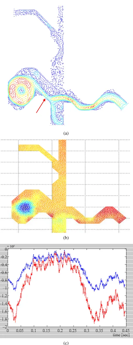
In order to demonstrate the potential of the CFD simulation technique, an example for such an (artificial) aneurysm is given in Figure 5, for which the velocity (Figure 5(a)) and pressure distributions (Figure 5(b))

(a)

(b)

(b) (c)

(a)

(b)

(c)

(d)

Figure 3. Simulated CFD data of the circle-of-willis vessel system, shown in Figure 2, if the boundary conditions are given by the velocity values of a real PCA measurement be- fore stenting: note the equal flow directions in the LPCOM (b) and RPCOM (c) which coincides with the results of the Nova data (d).

(b) (c)

(a)

(b)

(c)

(d)

(a)

(b)

(c)

Figure 5. CFD simulations of an artificial aneurysm. (a) The pressure distribution (b) and the forces (in dependence of time [sec]) (c) at the marked position (red arrow in a)) de- monstrate, that under special conditions the local load can achieve critical values, followed by a disrupture of the an- eurysm neck.

Table 1. Mean velocities within selected vessels in cm/sec.

Vessel LACA RACA LPCOM RPCOM LMCA RMCA

Before 42.61 13.35 7.93 42.77 26.32 30.47

After

Stent 55.70 29.29 10.71 27.62 30.88 29.62

are shown if physiologically reasonable boundary condi-tions are presumed. At the border of the area, indicated by the red arrow, the forces (Figure 5(c)) in x—(blue) and y—direction (red) are shown in dependence of time. The absolute values are not relevant in this case but merely the relative pressure and force enhancements at the neck of the aneurysm which finally may lead to a disrupture.

4. Discussion

CFD simulations were used to verify unexpected flow patterns that occur after stenting in the LPCOM vessel and to demonstrate the critical pressure and force distri- butions at the neck of an artificial aneurysm. The data shows that CFD simulations are feasible on comer- cially available PCs if the simulations are restricted to the es-sential vessel systems and if intrinsic symmetries are used to reduce the dimensionality of the problem. CFD data may also provide clinically useful information re- garding post-stenotic vessel wall alteration and progress- sion of atherosclerotic disease. More generally, wall shear stress is believed to play an important role in the evolu- tion of atherosclerosis and other arterial diseases, such as aneurysms.

At the current stage only vorticity but no turbulence model is implemented. Further CFD program options are different boundary conditions such as to extrapolate the boundary values of the pressure from the interior nodes or just to fix the value of the pressure at the outflow to zero.

The step from the TOF-MIP to a two-dimensional bit- map is currently not fully automated but necessitates ma- nual intervention by an experienced radiologist.

In future developments, a separate evaluation of dif- ferent heart phases will be possible as well. This deficit, however, does not lower the impact of the results, espe- cially because the flow directions before and after stent- ing do not depend on the heart phase.

In summarize, the intention of this work was to dem- onstrate, that the simulation of model based fluid dyna- mics provides important clinical information which is currently not available in most commercial software packages for flow quantification.

REFERENCES

“Three-Dimensional Phase Contrast Angiography,” Mag- netic Resonance in Medicine, Vol. 9, No. 1, 1989, pp. 139-149. doi:10.1002/mrm.1910090117

[2] G. K. Batchelor, “An introduction to Fluid Dynamics,” Cambridge University Press, Cambridge, 2000.

[3] E. Erturk, T. C. Corke and C. Gökçöl, “Numerical Solu- tions of 2-D Steady Incompressible Driven Cavity Flow at High Reynolds Numbers,” International Journal for Nu- merical Methods in Fluids, Vol. 48, No. 7, 2005, pp. 747- 774. doi:10.1002/fld.953

[4] D. Kim and H. Choi, “A Second-Order Time Accurate Fi- nite Volume Method for Unsteady Incompressible flow on Hybrid Unstructured Grids,” Journal of Computatio- nal Physics, Vol. 162, No. 2, 2000, pp. 411-428. doi:10.1006/jcph.2000.6546

[5] J. Kim and P. Moin, “Application of a Fractional Step Method to the Incompressible Navier-Stokes Equations,”

Journal of Computational Physics, Vol. 59, No. 2, 1985, pp. 308-323. doi:10.1016/0021-9991(85)90148-2

[6] A. Chorin, “Numerical Solution of the Navier-Stokes Equa- tions,” Mathematics of Computation, Vol. 22, No. 104, 1968, pp. 745-762.

doi:10.1090/S0025-5718-1968-0242392-2

[7] S. Armfield and R. Street, “Modified Fractional Step Me- thods for the Navier-Stokes Equations,” ANZIAM Journal, Vol. 45, 2004, pp. 364-377.

[8] S. Armfield and R. Street, “The Pressure Accuracy of Fractional Step Methods for the Navier-Stoke Equations on Staggered Grids,” ANZIAM Journal, Vol. 44, 2003, pp. 20-39.

[9] C. Rhie and R. Chow, “Numerical Study of the Turbulent Flow Past and Airfoil with Trailing Edge Separation,”

The American Institute of Aeronautics and Astronautics, Vol. 21, No. 11, 1983, pp. 1525-1532. doi:10.2514/3.8284

[10] http://www.cise.ufl.edu/~davis/

[11] C. W. Shu, “Total Variation Diminishing Time Discretisa- tions,” SIAM Journal onSociety and Scientific Comput- ing, Vol. 9, No. 6, 1988, pp. 1073-1084.

doi:10.1137/0909073

[12] P. J. Roache, “Quantification of Uncertainty in Computa- tional Fluid Dynamics,” Annuls Reviews of Fluid Me- chanics, Vol. 29, 1997, pp. 123-160.

doi:10.1146/annurev.fluid.29.1.123