A Simple Explanation for the Higgs Mechanism Given by a Modified Kronig Penney Model

(1)

ISSN Online: 2380-4335 ISSN Print: 2380-4327

DOI: 10.4236/jhepgc.2019.54064 Oct. 8, 2019 1112 Journal of High Energy Physics, Gravitation and Cosmology

A Simple Explanation for the Higgs-Mechanism

Given by a Modified Kronig-Penney-Model

Carsten Wochnowski

Karlsfeld, Germany

Abstract

In this paper the Higgs mechanism is simply explained by a modification of the Kronig-Penney-Model well known in solid state physics. By this model an inverse (harmonic) oscillator is derived which can give a hint to Higgs Me-chanism, eventually the Higgs Mechanism can be explained by this modified Kronig-Penney-Model. Also a short explanation is given for the relativistic curvature of space by the presence of mass and for the Heisenberg uncertain-ty principle.

Keywords

Higgs Mechanism, Kronig-Penney-Model, Space and Time Quantization, Heisenberg Uncertainty Principle, Copenhagen Interpretation,

De Broglie-Bohm Theory

1. Introduction

Modified Kronig-Penney model

In [1] a modified Kronig-Penney model has been presented relating to the unified field theory:

It has been assumed that space and material are quantised: the space is subdi-vided by an array of equidistantly arranged Delta potentials forming space quanta (space quantisation). If a material quantum is inserted into this Delta potential array, the solution of the Schrödinger equation yields the formula [1]:

(

)

2

(

)

0

kin E E x na

zV

ψ = = − ₍₁₎

with ψ

(

x na=

)

2_{as the material quantum probability density distribution at} the sites x na= of the Delta potential in space, E as the total energy of the ma-terial quantum, Ekinas the kinetic energy of the material quantum, z as the

num-How to cite this paper: Wochnowski, C. (2019) A Simple Explanation for the Higgs-Mechanism Given by a Modified Kronig-Penney-Model. Journal of High Energy Physics, Gravitation and Cosmolo-gy, 5, 1112-1122.

https://doi.org/10.4236/jhepgc.2019.54064

Received: August 19, 2019 Accepted: October 5, 2019 Published: October 8, 2019

http://creativecommons.org/licenses/by/4.0/

(2)

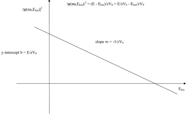
DOI: 10.4236/jhepgc.2019.54064 1113 Journal of High Energy Physics, Gravitation and Cosmology ber of Delta potentials in this model and V0 as a pre-factor of the Delta potential. The material quantum probability distribution ψ

(

x na=

)

2 is drawn against Ekin (Figure 1; in [1] this figure is also denoted as Figure 1(a)).

[image:2.595.209.539.288.488.2]

It has been shown that two solutions are the most relevant ones: in case of the first solution, the mterial quantum probability density distribution is located ex-actly between two Delta potentials and hence precisely in the center of a space quantum: in this state the material quantum can be interpreted as a mass quan-tum (Figure 2(a), in [1] this figure is also denoted as Figure 2(a)), while in case of the second solution the material quantum probability density distribution is located exactly at the sites of the Delta potentials, and hence at the lateral area of a space quantum: in this state the material quantum can be interpreted as an energy quantum or photon (light) (Figure 2(b); in [1] this figure is denoted as Figure 2(f)).

Figure 1. The material quantum probability density |ψ(x = na, Ekin)|2 is drawn against the

kinetic energy Ekin yielding a linear graph with the slope of −1/zV0 and an y-intercept of

E/zV0.

(a) (b)

Figure 2. (a) The first relevant solution of Schrödinger equation yields that the material

[image:2.595.214.535.544.644.2]

(3)

DOI: 10.4236/jhepgc.2019.54064 1114 Journal of High Energy Physics, Gravitation and Cosmology The material quantum behaviour inside the Delta potential array can be in-terpreted as a vibration state faintly similar to a string. The array of Delta poten-tials can be considered faintly as something similar to the Higgs field.

This modified Kronig-Penney model can also be applied to Solid State Physics [2].

Higgs mechanism (strongly simplified illustration)

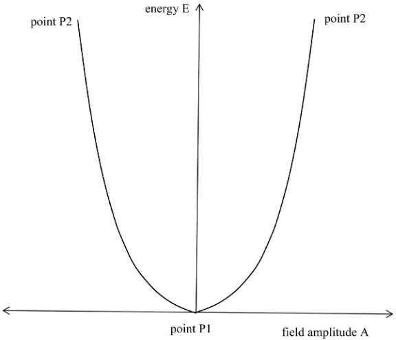
The potential curve of a harmonic oscillator is shown in Figure 3: the energy E is drawn against the oscillation field amplitude A with E ~ A2_{. It is evident that} at the point P1 (in Figure 3) the energy E is zero and also the oscillation field amplitude A is zero, while at the points P2 (in Figure 3) the energy E is larger than zero and the oscillation field amplitude A is also larger than zero. This matches with our daily-life experience.

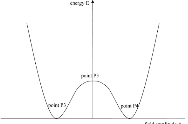
[image:3.595.229.517.446.693.2]

In case of an oscillator subject to a Higgs potential, the situation is vice versa and more complex which is illustrated in a very simplified way as follows: In Figure 4 the potential curve of a Higgs oscillator is shown. Again the energy E is drawn against the oscillating field amplitude A. The Higgs potential is characte-rized by two minima (in Figure 4 denoted by point P3 and point P4) and a local maximum (in Figure 4 denoted by point P5), so the Higgs potential looks like a Mexican hat or donut profile. This can be interpreted as follows: at point P3 and point P4 the energy E is zero, but the oscillation field amplitude A is larger than zero; that means the Higgs oscillator is oscillating or vibrating, although the energy E is zero. At point P5 the energy E is larger than zero, but the oscillation field amplitude A is zero; that means the Higgs oscillator is not oscillating or vi-brating, although the energy E is larger than zero.

Figure 3. Potential curve of a harmonic oscillator by which the energy E is drawn against

(4)

[image:4.595.215.534.74.284.2]

DOI: 10.4236/jhepgc.2019.54064 1115 Journal of High Energy Physics, Gravitation and Cosmology

Figure 4. An oscillator featured by a Higgs potential (energy E drawn against the field

amplitude A) with two local minima (points P3 and P4: energy E = 0, while field oscilla-tion amplitude A > 0) and a local maximum (point P5: energy E > 0, while field oscilla-tion amplitude A = 0).

This strange oscillation or vibration behavior can be considered as an inverse (harmonic) oscillator, and indeed the area between the point P3 and P4 can be approximately seen as an inverse potential curve of a harmonic oscillator. This strange oscillation or vibration behavior can be explained by a modified Kro-nig-Penney Model originally conceived in Solid State Physics and now applied to the Higgs mechanism in this paper.

2. Theoretical Contemplation

(5)

maxi-DOI: 10.4236/jhepgc.2019.54064 1116 Journal of High Energy Physics, Gravitation and Cosmology mum at the center and minimum at the side lines as above discussed, while at high (kinetic) energy the probability distribution density |ψ(x)|2_{is minimum at} the center and maximum at the side lines (or to be more precisely: in the mo-mentary state of maximum kinetic energy, |ψ(x)|2_{is minimum at center and in} the momentary state of maximum potential energy, |ψ(x)|2_{is maximum at the} side lines).

As already stated above, in case of a Higgs oscillator the field amplitude A is zero at an energy E > 0 (point P5 in Figure 4), while the field amplitude A is larger than zero at an energy E = 0 (points P3 and P4 in Figure 4). This means vibration or oscillation occurs at an energy E = 0 (see points P3 and P4 in Figure 4), while no vibration or no oscillation occurs at an energy E > 0 (see point P5 in Figure 4).

Obviously, one can easily observe that between the points P3 and P4 the Higgs potential is similar to an inverse harmonic oscillator.

This kind of vibration behaviour is similar to the inverse (harmonic) oscillator being based on the modified Kronig-Penney-Model as discussed [1]. Thus is can be assumed that the inverse (harmonic) oscillator being based on the Higgs po-tential is similar to the inverse (harmonic) oscillator being based on the modified Kronig-Penney-Model (or being based on an equidistant array of Delta poten-tials). Eventually by this way the Higgs Mechanism can be explained by the modified Kronig-Penney-Model, while the Higgs field is nothing else as a peri-odic array of Delta potentials equidistantly arranged from minus infinity to plus infinity in which material quanta occur.

Something similar to an inverse oscillator can be often found in solid state physics: the dispersion relation of a free electron is parabolic, but inside a crystal lattice the periodic and regular arrangement of positively charged atomic nuclei has a huge impact of the electron movement subject to dispersion relation inside the crystal lattice (often the dispersion relation of an electron inside a solid state crystal lattice deviates from the parabolic form, e.g. the effective mass of an elec-tron can even become negative) [3] [4] [5] [6].

Such kind of an inverse oscillator can be illustrated in a very descriptive way: an attractive interaction exists between the material quantum and the adjacent Delta potentials. Thus the resting position (Ekin = 0) of such an inverse oscillator is shown in Figure 2(b), when the material quantum is located around the Delta potential, that means ψ

(

x na=

)

2 is maximal at the sites of the Delta poten-tials (corresponding to the point of intersection between graph and axis of ordi-nates in Figure 1). In this position the material quantum has a minimal kinetic energy and it is in a stable equilibrium state, because the attractive interaction between the material quantum and the Delta potential makes the material quantum being fixed at the Delta potential.

The position as shown in Figure 2(a) (corresponding to the point of intersec-tion between graph and axis of abscissa in Figure 1), when the material quan-tum is located exactly between two adjacent Delta potentials (that means

(

)

2

x na

(6)

DOI: 10.4236/jhepgc.2019.54064 1117 Journal of High Energy Physics, Gravitation and Cosmology state with a maximal kinetic energy Ekin), is also an equilibrium state, but not a stable or indifferent one, but rather an unstable or labile one: only exactly in this position the material quantum is submitted to the same attractive interactions exerted by the Delta potentials from both sides. Already a slight displacement can destroy the instable equilibrium state. Between both equilibrium states, the stable and the unstable or labile one, only a non-equilibrium intermediate state could eventually occur which only temporarily exits or even which eventually must not exist at all, because it is forbidden. Thus the energy gap is explained in a descriptive way separating a mass quantum and an energy quantum from one another.

By further contemplation one can draw the following two conclusions from the precedent passage:

Firstly, the movement of a material quantum through the array of Delta po-tentials are not continuously, but discrete or quantized, otherwise the material quantum must take temporarily the non-equilibrium intermediate state (which is eventually forbidden), when it is moving from one cubic space quantum cell to the other. This can only explained by time quantization: In case of time quanti-zation only two states exists: the material quantum is in the cubic space quantum cell A or the material quantum is in the adjacent cubic space quantum cell B, while no intermediate state exists. Thus the movement of the material quantum takes place step-by-step or to be more precisely, the migration of the material quantum is quantized.

(7)

(a)

(b)

[image:7.595.275.470.69.534.2]

(c)

Figure 5. (a) A cubic space quantum cell with no material quantum present has a length

of a; (b) Now a material quantum is inserted precisely in the center of the cubic space quantum cell having an exact distance of a/2 towards the two Delta potentials on both sides; the material quantum is subject to the attractive interactions with the neighbouring Delta potentials on both sides compensating each other, thus the material quantum does not move (unstable equilibrium state); (c) The attractive interactions between the materi-al quantum and the two Delta potentimateri-als are not one-sided, but both-sided materi-also having an impact on the site of the Delta potentials (see two additional arrows in the (c)), thus making the two Delta potentials shifting to the center of the space quantum cell where the material quantum is located: the length of the space quantum cell reduces from a to a*.

(8)

DOI: 10.4236/jhepgc.2019.54064 1119 Journal of High Energy Physics, Gravitation and Cosmology quantum cell is reduced from the value a to a* due to the Delta potential shift described above, which can be interpreted as space curvature (Figure 5(c)). That means that the two adjacent Delta potentials are now separated by a distance a* from one another, if the material quantum occurs precisely in the center of the cubic space quantum cell, and which is smaller to the space quantum cell length a > a* in case of no material quantum is present inside the space quantum cell.

If one consider the state of the material quantum located in the center of the space quantum cell as a mass quantum (as shown in Figure 2(a) or Figure 5(b) and Figure 5(c)), one can interpreted this kind of space deformation as the space curvature in the presence of mass according to Einstein general theory of relativ-ity. Thus the relativistic space curvature is nothing else than the Delta potentials’ shift towards the material quantum (located at the center of the cubic space quan-tum cell) due to attractive interaction between material quanquan-tum and Delta po-tentials.

3. Conclusions

Both the space curvature of the space quantum cell (due to the presence of mass quantum) and the time quantization lead to the Heisenberg’s uncertainty prin-ciple: the probability density distribution |ψ|2_{of a particle depends on the} se-quence of space quanta occupation by mass quantum shown by a simple Monte Carlo simulation:

At first we observe three adjacent cubic space quantum cells side by side (Figure 6(a)): the left one is denoted by SQ1, the middle one is denoted by SQ2 and the right one is denoted by SQ3. At the beginning all three cubic space quantum cells are empty or unoccupied, which means all three space quantum cells are not occupied by any material quantum. All space quantum cells have a length of a (Figure 6(a)). The initial position of the entire space quantum cell triplet is located in the middle.

(9)

(a)

(b) (c)

(d) (e)

[image:9.595.216.534.69.392.2]

(f) (g)

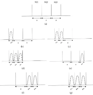
Figure 6. (a) Three empty adjacent cubic space quantum cells SQ1, SQ2 and SQ3 not

oc-cupied by a material quantum; each space quantum cell has a length of a, respectively; (b) and (c) Now the subsequent occupation of the space quantum cells starts from the left side; the length of an occupied space quantum cell reduces from a to a*; (d) After the subsequent space quantum cell occupation has finished from the left side, all space quan-tum cells are occupied and have a length of a*, respectively; the space quanquan-tum cell triple has shifted to the left; (e) and (f) Now the subsequent occupation of the space quantum cells starts from the right side; (g) After the subsequent space quantum cell occupation has finished from the right side, all space quantum cells are occupied (as it is the case in (d)) and all space quantum cells have a length of a*, respectively; but the space quantum cell triple has shifted to the right in contrast to (d).

time quant later the middle space quantum cell SQ2 is occupied also implying a reduction of the cell length from a to a* (Figure 6(f)). Thus the space quantum triple is further shifted to the right side. After all a time quant later the left space quantum cell is occupied SQ1 at last also implying a reduction of the cell length from a to a* (Figure 6(g)). This sequence of space quantum cell occupation by a mass quantum results in a shift of the entire space quantum triple to the right side.

(10)

DOI: 10.4236/jhepgc.2019.54064 1121 Journal of High Energy Physics, Gravitation and Cosmology the entire space quantum cell triple. Evidently, the final position of the entire space quantum triple strongly depends on the order by which the space quan-tum cells are occupied by the material quanta.

By processing this Monte Carlo simulation, all possible occupation orders or occupation sequences can be simulated: so one can start the occupation order by occupying firstly the middle space quantum cell SQ2 and then the left or right space quantum cell, etc.

By performing a Monte Carlo simulation with much more than three space quantum cells, it can be shown that a probability density distribution of the final position of the entire space quantum n-tuple exists with a maximum in the cen-ter and inclining flanks to the sides, similar to a Gaussian exponential function as discussed as follows:

Although it is not mathematically completely correct, this kind of Monte Car-lo simulation experiment can be approximated by a Poisson binomial distribu-tion with its probability mass funcdistribu-tion ρX(k):

( )

(

1

)

X k pi pj

ρ =

∑∏ ∏

− (2)

with ρX(k) as the probability of having k successful trials and pi and pj as the probability of the trials i and j, respectively.

The corresponding distribution function F kX

( )

=P X k

(

≤

)

is as follows:

( )

(

)

(

1

)

X k i j

F k =P X k≤ =

∑ ∑∏ ∏

p −p (3) with F kX

( )

=P X k

(

≤

)

as the probability of having X successful trials between

0 and k.

According to [7], the Poisson binomial distribution FX(k) itself can be ap-proximated by the normal distribution function φ

( )

k _{in case of a large number} of trials:

( )

0.5

X k

F k φ µ

σ

+ −

 

≈ _ _ (4)

with μ as the expected value and σ as the standard deviation.

Summarizing, consequently the final position of the entire space quantum triple strongly depends on the occupation sequence of the space quantum cells by the material quanta that means it depends in which order the space quantum cells are occupied by the material quanta. This could be interpreted as the Hei-senberg’s uncertainty principle.

Of course it can be happen that during a single time quant, all space quantum cells are being occupied simultaneously, but this is very unlikely to happen al-though it cannot be totally excluded.

This interpretation combines elements of De-Broglie-Bohm theory and ele-ments of Copenhagen interpretation of Quantum mechanics with one another.

Conflicts of Interest

(11)

References

[1] Wochnowski, C. (2019) A Very Simple Model Concerning the Unified Field Theory Basing on the Kronig-Penney-Model. Journal of High Energy Physics, Gravitation and Cosmology, 5, 941-952. https://doi.org/10.4236/jhepgc.2019.53050

[2] Wochnowski, C. (2019) A Novel Theoretical Derivation for the Existence of an Energy Band Gap in a Perfect Solid State Crystal Lattice. Frontiers of Science and Theory, 1, 5-16.

http://intrepidpublishingllc.com/frontiers-of-science-and-theory/volume-i-issue-ii/

[3] Kittel, C. (2002) Einführung in die Festkörperphysik. de Gruyter, Berlin. [4] Ibach, H. and Lüth, H. (2009) Festköperphysik. Springer, Berlin.

[5] Bonc-Bruevic, V.L. and Kalasnikov, S.G. (1982) Halbleiterphysik. VEB Verlag, Ber-lin. https://doi.org/10.1007/978-3-7091-9495-9

[6] Ashcroft, N.W. (1976) Solid State Physics. Brooks Cole, Monterey.

[7] Hong, Y. (2011) On Computing the Distribution Function for the Sum of Indepen-dent and Non-IIndepen-dentical Random Indicators. Blacksburg, USA.