The Effectiveness of the Squared Error and Higgins Tsokos Loss Functions on the Bayesian Reliability Analysis of Software Failure Times under the Power Law Process

(1)

ISSN Online: 1947-394X ISSN Print: 1947-3931

DOI: 10.4236/eng.2019.115020 May 23, 2019 272 Engineering

The Effectiveness of the Squared Error and

Higgins-Tsokos Loss Functions on the Bayesian

Reliability Analysis of Software Failure Times

under the Power Law Process

Freeh N. Alenezi

1,2

, Christ P. Tsokos

1

1_{University of South Florida, Tampa, FL, USA} 2_{Majmaah University, Al-Zulfi, Saudi Arabia}

Abstract

Reliability analysis is the key to evaluate software’s quality. Since the early 1970s, the Power Law Process, among others, has been used to assess the rate of change of software reliability as time-varying function by using its intensity function. The Bayesian analysis applicability to the Power Law Process is jus-tified using real software failure times. The choice of a loss function is an im-portant entity of the Bayesian settings. The analytical estimate of likelih-ood-based Bayesian reliability estimates of the Power Law Process under the squared error and Higgins-Tsokos loss functions were obtained for different prior knowledge of its key parameter. As a result of a simulation analysis and using real data, the Bayesian reliability estimate under the Higgins-Tsokos loss function not only is robust as the Bayesian reliability estimate under the squared error loss function but also performed better, where both are supe-rior to the maximum likelihood reliability estimate. A sensitivity analysis re-sulted in the Bayesian estimate of the reliability function being sensitive to the prior, whether parametric or non-parametric, and to the loss function. An interactive user interface application was additionally developed using Wol-fram language to compute and visualize the Bayesian and maximum likelih-ood estimates of the intensity and reliability functions of the Power Law Process for a given data.

Keywords

Power Law Process, Bayesian Reliability, Intensity Function, Kernel Density, Loss Function, Robustness

How to cite this paper: Alenezi, F.N. and Tsokos, C.P. (2019) The Effectiveness of the Squared Error and Higgins-Tsokos Loss Functions on the Bayesian Reliability Analy-sis of Software Failure Times under the Power Law Process. Engineering, 11, 272-299.

https://doi.org/10.4236/eng.2019.115020

Received: April 24, 2019 Accepted: May 20, 2019 Published: May 23, 2019

(2)

DOI: 10.4236/eng.2019.115020 273 Engineering

1. Introduction

Reliability analysis of a software under development is a key to assess whether a desired level of a quality product is achieved. Specially, when a software package is considered, and is tested after each failure detection, and then corrected until a new failure is observed. Over the past few decades, the reliability analysis of a software package has been studied, where graphical and numerical metrics have been introduced. One of the earliest, Duane (1964) [1], who introduced a graph to assess the reliability of a software over time using its failure times. It has the cumulative failure rate and the time on the y-axis and x-axis, respectively. In this graph, one can conclude a software reliability improvement if a negative curve is observed whereas a positive curve means the software reliability is deteriorating. On the other hand, a horizontal line indicates that the software reliability is stable. The failure numbers N t

( )

in time interval

(

0,t

]

is considered a Poisson counting process after satisfying the following conditions:

1) N t

(

=0

)

=0.

2) Independent increment (counts of disjoint time intervals are independent). 3) It has an intensity function

( )

lim₀

(

,

)

1

)

.

t

P N t t t

V t

t

∆ →

+ ∆ = =

∆

4) Simultaneous failures do not exist

(

)

(

)

0

, 2

lim_t P N t t t 0.

t

∆ →

+ ∆ = = ∆

The probability of random value N t

( )

=n is given by:

( )

(

)

exp

{

0

( )

d

}

{

0

( )

d

}

, 0. !

n

t t

V t t V t t

P N t n t

n −

= =

∫

> ₍₁₎

Crow (1974) proposed a Non-Homogeneous Poisson Process (NHPP) , which is a Poisson Process with a time varying intensity function, given by:

( )

(

; ,

)

t 1, 0, 0, 0,

V t V t t

β

β θ

β

θ

θ θ

−  

= = _{ } > > >

  (2)

with β and θ are the shape and scale parameters, respectively. This Non- Homogeneous Poisson Process is also known as the Power Law Process (PLP).

The joint probability density function (PDF) of the ordered failure times 1, , ,2 n

T T T from a NHPP with intensity function V t

(

; ,

β θ

)

is given by:

(

1, ,

)

1

(

; , exp

)

{

0

(

; , d ,

)

}

w n

n i i

f t t =

∏

₌V t β θ −

_∫

V t β θ t (3) where w is the so-called stopping time; w t= n for the failure truncated case.

Considering the failure truncation case, the conditional reliability function of the failure time Tn given T t1= 1, T2 =t2, T3=t3,

, Tn−2=tn−2, Tn−1=tn−1 is a function of V t

(

; ,

β θ

)

.

(3)

(

; ,

)

V t

β θ

has an important role in evaluating the reliability of a software package. When the estimates of β_{are less and larger than 1, they indicate that}

the software reliability is improving and decreasing, respectively. The PLP is reduced to a homogeneous Poisson process when the estimate of β equals to 1.

The NHPP has been used for analyzing software’s failure times, and prediction of the next failure time. The subject model has been shown to be effective and useful not only in software reliability assessment [2]-[11], but also in cyber- security; the attack detection in cloud systems [12] [13], breast and skin cancer treatments’ effectiveness, [14] [15] [16], respectively, finance; modeling of financial markets at the ultra-high frequency level [17], trnasportation; modeling passengers’ arrivals [18] [19] [20] [21] [22], and in the formulation of a software cost model [23].

Since the conditional reliability function of the PLP is a function of the

(

; ,

)

V t

β θ

, which includes the key parameter β. That being said updating the estimation methods for the key parameter will affect positively the V t

(

; ,

β θ

)

and the software reliability estimation, and therefore help the structuring of maintenance strategies. The authors [24] and [25] obtained the Bayesian estimates of the parameter β under the the squared-error and Higgins-Tsokos loss functions, respectively, and compared them to their approximate maximum likelihood estimate (MLE). They also showed the superiority of the Bayesian estimates to the MLE of the key parameter β, and the improvement in the reliability assessment under the PLP.

To perform Bayesian analysis on a real world problem, one needs to justify the applicability of such analysis. Then, the analysis process starts by identifying the probability distribution of the failure times of a software under development, the prior PDF of the key parameter β , and a loss function. The analytical tractability have made the squared-error loss function commonly used, where it places more weight on the estimates that are far from the true value than the estimates close to true value. Higgins and Tsokos [26] proposed a new loss function that maintains the analytical tractability feature and places exponentially more weight on extreme estimates of the true value.

In the present study, we investigate the effectiveness, in Bayesian Analysis, of using the commonly used squared-error (S-E) loss function versus the Higgins- Tsokos (H-T) loss function that puts the loss at the end of the process, for modeling software failure times. To accomplish this, we used the underline failure distribution to be the Power Law Process subject to using Burr PDF as a prior of the key parameter β. In addition, we utilize both loss functions to perform sensitive analysis of the prior selections. We perform parametric and non-parametric priors, namely Burr, Inverted Gamma, Jeffery, and two Kernel PDFs. Therefore, the primary objective of the study is to answer the following questions within a Bayesian framework:

(4)

challenged by the Higgins-Tsokos loss function in estimating the key parameter

β of PLP for modeling software failure times?

2) Is the Bayesian estimate of the intensity function, V t

(

; ,

β θ

)

, of the PLP sensitive to the selections of the prior (parametric and non-parametric) and loss function (Higgins-Tsokos and S-E loss functions)?

The paper is organized as follows, Section 2 describes the theory and development of the Bayesian reliability model. Section 3 presents the results and discussion. Section 4 are the conclusions.

2. Theory and Bayesian Estimates

2.1. Review of the Analytical Power Law Process

The probability of achieving n failures of a given system in the time interval

(

0,t

]

can be written as

(

)

exp

{

0

( )

d

}

{

0

( )

d

}

; , 0,

!

n

t t

V x x V x x

P x n t t

n −

= =

∫

> (4)

where V t

( )

is the intensity function given by (2). The reduced expression is given by:

(

;

)

1exp ,

!

n

t t

P x n t n

β β

θ θ

 

 

= = _− _

 

  (5)

is the PLP that is commonly known as Weibull or Non-Homogeneous Poisson Process.

When the PLP is the underlying failure model of the failure times 1 2 3, , , , n1

t t t t − and tn, the conditional reliability function of tn given

1 2 3, , , , n1

t t t t − can be written mathematically as a function of the intensity

function, given by:

(

)

{

(

)

}

1

1 2 1 1

| , , , exp n ; , d , 0,

n

t

n n _t n n

R t t t t V t β θ t t t

−

− =

∫

− > − >

(6)

since it is independent of t t t1 2 3, , , , tn−2.

Note that the improvement in estimating the key parameter β in the

(

n| , , ,1 2 n1

)

R t t t t − of the PLP, Equation (6), will improve the reliability esti-

mation.

The maximum likelihood estimation (MLE) of β_{is a function of the largest}

failure time and the MLE of θ is also a function of the MLE of β. Let 1, , ,2 n

T T T denote the first n failure times of the PLP, where T Tl< 2<<Tn

are measured in global time; that is, the times are recorded since the initial startup of the system. Thus, the truncated conditional probability distribution function, f t ti

(

| , ,1ti−1

)

, in the Weibull process is given by

(

)

1 1

1 1 1

| , , exp i , .

i i t t t i

f t t t t t

β β β

β

θ θ

θ

−

− −

 

 

 

=  _{ } − +  <

 

 

(5)

With t=

(

t t1 2, ,. , tn

)

, the Likelihood function for the first n failure times of

the PLP T t T1= 1, 2=t2, , Tn =tn can be written as

( )

1

, exp n n n i .

i

t t

L t

β β

β

θ

−

=

 _{ } _{ } _{ }

= _−_{ } _{ } _{ }

 

   

 

∏

(8)

The MLE for the shape parameter is given by

1

ˆ _,

log

n

n _n

i i

n t t

β

= =

     

∑

(9)

and for the scale parameter is

ˆ 1

ˆ _.

n

n t

n β

θ = (10) Note that the MLE of θ depends on the MLE of β.

2.2. Development of the Bayesian Estimates

The authors [24] and [25] justified the applicability of Bayesian analysis to the PLP based on the Crow, [2] [27], failure data from a system undergoing developmental testing (Table 1), by showing that the MLE of the key parameter

β varies depending on the last failure time (largest time). Moreover, the authors used the Crow data (40 successive failure times) to compute the MLE of

β (

β

ˆ40=0.49), then computed the estimate considering the t39 =3181 is the largest failure time (

β

ˆ39=0.48) and so on. After computing all MLEs of the key parameter β, they found that the MLEs of β follows a four-parameter Burr probability distribution, g

(

β α γ δ κ

; , , ,

)

, known as the four-parameter Burr type XII probability distribution, with a PDF given by:

( )

(

)

1 1

; , , ,

1

0 otherwise

B

g g

α

κ α β γ ακ

δ _{γ β}

β β α γ δ κ _{β γ}

δ

δ −

+

 _ ₋ _

 _ _

 _{≤ < ∞}

  

= _{= } _ ₋ _

+

   

 _ _ _ _ 



(11)

[image:5.595.199.540.611.741.2]

where the hyperparameters α, γ , δ _and

κ

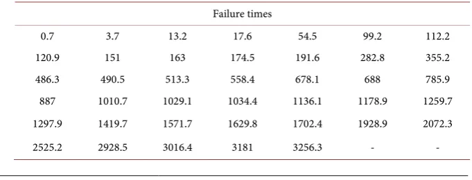
are being estimated using MLEs in the Goodness of Fit (GOF) test applied to the β_{estimates. The MLE}

Table 1. Crow’s failure times of a system under development.

Failure times

(6)

of the key parameter β is always affected by the largest failure, and therefore it is recommended not to consider it unknown constant. This recommendation provides the opportunity to study Bayesian analysis in the PLP with respect to various selections of loss functions and priors.

The Bayesian estimates of β will be derived using the squared-error and Higgins-Tsokos loss functions.

2.2.1. Bayesian Estimates Using Squared Error (S-E) Loss Function

The S-E loss function is given by:

( ) ( )

_ˆ

2

,

.

L

ξ ξ

=

ξ ξ

−

₍₁₂₎

The risk using the S-E loss function, where ξ β= represents the estimate of

ˆ ˆ

ξ β

= , is given by:

( )

ˆ_,

(

ˆ

)

2

(

_{| d ,}

)

E L_

β β

 =_ _−∞∞ _

β β

− _h

β

t

β

 

∫

(13)

By differentiating

E L



_

( )

β β

ˆ,



_

_{with respect to}β and setting it equal to zero we solve for

β

ˆ, the Bayesian estimate of β with respect to the S-E loss function and Burr probability distribution, Equation (11), given by:

(

)

.

ˆ _{| d ,}

B SE h t

β =

_∫

_−∞∞β⋅ β β (14) where the posterior PDF of β given data (t), h

(

β

|t

)

, using the Bayes?€? theorem, is given by:

(

)

(

) ( )

(

) ( )

| | . | d B B

L t g

h t

L t g

β β

β

β β β

∞ −∞ =

∫

(15)

Then, the Bayesian estimate of β, under the squared-error loss, is given by 1 1 1 1 1 . 1 1 1 1 exp d 1 ˆ _. exp d 1 n n n i n i B SE n n n i n i t t t t α β β κ γ α α β β κ γ α β γ

β δ _β

θ θ

θ _{β γ}

δ β

β γ

β δ _β

θ θ

θ _{β γ}

δ − − + ∞ + = − − ∞ + = −       ₋         _{ }   _{ }       _ ₊ −  _    _ _    = −       ₋         _{ }   _{ }       _ ₊ −  _    _ _   

∏

∫

∏

∫

(16)

2.2.2. Bayesian Estimates Using the Higgins-Tsokos Loss Function

The H-T loss function (1976) is given by

( )

1

{

2

(

)

}

2

{

1

(

)

}

1 2

ˆ ˆ

exp exp

ˆ, f f f f 1, , 0.

L f f

f f

ξ ξ ξ ξ

ξ ξ = − + − − − >

+ (17)

(7)

ˆ ˆ

ξ β

= _{, is given by:}

( )

1

{

2

(

)

}

2

{

1

(

)

}

(

)

1 2

ˆ ˆ

exp exp

ˆ, f f f f 1 | d

E L h t

f f

β β β β

β β _−∞∞ β β

 ₋ ₊ ₋ ₋     _{ =} ₋     ₊    

∫

(18)

By differentiating

E L



_

( )

β β

ˆ,



_

_{with respect to}β and setting it equal to zero we solve for

β

ˆ, the Bayesian estimate of β_{with respect to the H-T loss}

function, given by:

{ } (

)

{

} (

)

1 .

1 2 ₂

exp | d

1

ˆ _ln _.

exp | d

B TH

f h t

f f _f _h _t

β β β

β

β β β

∞ −∞ ∞ −∞     = _ _ + ₋  

∫

(19)

The Bayesian estimate of β with respect to the Higgins-Tsokos loss function and Burr probability distribution, as the prior, has h

(

β

|t

)

given by

(

)

1 1 1 1 1 1 1 1 exp d 1 | . ( ) exp d 1 n n n i i n n n i i t t h t t t α β β κ α α β β κ γ α β γ

β δ _β

θ θ θ _{β γ}

δ

β _{β γ}

β _δ _β

θ θ θ _{β γ}

δ − − + = − − ∞ + = −               ₋                   _ ₊ −  _    _ _    = −           ₋                 _ ₊ −  _    _ _   

∏

∫

(20)

With the use of Equation (6), the conditional reliability of

t

i, the analytical

structure of the conditional Bayesian reliability estimate for the PLP that is subject to the above information is given by:

(

)

{

(

)

}

1

1 2 1 1

ˆ _{| , , ,} _exp i ˆ _{; , d ,} _0,

i

t

B i i _t B i i

R t t t t V t β θ t t t

−

− = −

∫

′ > − >

(21) where

(

)

* * * ˆ 1 ˆ ˆ

ˆ ; , B B , 0, 0,

B _B t

V t t

β β

β θ θ

θ θ −  

′ = _{ } > >

  (22)

where

β

ˆ_B* is the Bayesian estimate using

β

ˆB SE. or

β

ˆB TH. for the squared error or Higgins-Tsokos loss functions, respectively. We are also interested in comparing the Bayesian estimates, using Higgins-Tsokos loss function, of the subject parameter for different parametric and non-parametric priors, and with respect to its MLE given by Equation (9), assuming β has a random behavior and θ as known; as well as, comparing Equation (10) with an adjusted MLE considered as a function of β.

2.3. Sensitivity Analysis: Prior and Loss Function

(8)

using simulated data, sensitive analysis was done for the following parametric and non-parametric priors ([25]):

1) Jeffreys’ prior ([28]): Jeffreys’ prior is proportional to the square root of the determinant of the Fisher information matrix (I

( )

β

). It is a non-informative prior, where the Jeffreys?€? prior for the key parameter of the PLP I

( )

β

is scalar in this case, is given by:

( )

2log ₂

( )

; 1 , 0.

J

L t

g

β

I

β

E

β

∂ 

∝ = − _ _∂ _∝ >

  (23)

2) The inverted gamma: The PLP and inverted gamma probability distributions belong to the exponential family of probability distributions, which makes the latter a logical choice for an informative parametric prior for β. The inverted gamma probability distribution is given by:

( )

1 1 exp

_{( )}

, 0, 0, 0,

v

IG

g v

v

µ µ

β β µ

β µ β

+

  − 

∝_{ } _ _ > > >

Γ

    (24)

where v and µ_{are the shape and scale parameters.}

3) Kernel’ prior:

The kernel probability density estimation is a non-parametric method to approximately estimate the PDF of β using a finite data set. It is given by:

( )

1

1 n _,

i K i g K nh h

β β

β

= −   = _ _  

∑

(25)

where K is the kernel function and h is a positive number called the bandwidth.

2.3.1. The Jeffreys’ Prior

Assuming Jeffreys’ PDF (23) as the prior of β and using the likelihood (8) and (15), the posterior density of β_is:

(

)

( )

1 ₁ 1 1 ₁ 1 0 exp | . exp d n n n i n i J _n n n i n i t _t h t t _t β β β β β β β θ θ β β _β θ θ − − = − ∞ − =       _{ }      =       _{ }     

∏

∫

(26)

Thus, the Jeffreys’ Bayesian estimate of the key parameter β under the S-E and H-T loss functions, using (14) and (19), are given by:

(

)

. ₀

ˆJ _| _{d ,}

B SE h tJ

β =

_∫

∞β⋅ β β (27) and

{ } (

)

{

} (

)

1 0 .

1 2 ₂

0

exp | d

1

ˆ _ln _.

exp | d

J J

B HT

J

f h t

f f _f _{h t}

β β β

β

β β β

∞ ∞     = _ _ + ₋  

∫

(28)

(9)

DOI: 10.4236/eng.2019.115020 280 Engineering 2.3.2. The Inverted Gamma Prior

The following is an examination of the problem when the prior density of β is given by the inverted gamma (24). Using the likelihood (8), the posterior density of β is given by:

(

)

( )

1 ₁ 1 1 ₁ 1 0 exp | . exp d n v n n i n i

IG _{n v}

n n i n i t _t h t t _t β β β β β β β µ θ β θ β

β µ _β

θ β θ − − ₋ = − − ∞ − =   ₋  ₋    _{ }      =   ₋  ₋    _{ }     

∏

∫

(29)

Thus, the Bayesian estimates of β under the inverted gamma with respect to the S-E and H-T loss functions, using (14) and (19), are given by:

(

)

. ₀

ˆIG _| _{d ,}

B SE hIG t

β =

_∫

∞β⋅ β β (30) and

{ } (

)

{

} (

)

1 0 .

1 2 ₂

0

exp | d

1

ˆ _ln _.

exp | d

IG IG

B HT

IG

f h t

f f _f _{h t}

β β β

β

β β β

∞ ∞     = _ _ + ₋  

∫

(31)

Here as well, we must rely on a numerical estimation because we cannot obtain close solutions for

β

ˆB SEIG. and

β

ˆB HTIG. . Also note that it depends on knowing or being able to estimate the scale parameter θ.

2.3.3. The Kernel Prior

Assuming Kernel density (25) as the prior of β and using the likelihood (8), the posterior density of β is:

(

)

( )

1 1 1 1 1 1 0 1 exp | . 1 exp d n n n n i i

n i i

k _n

n n

n i

i

n i i

t _t _K

nh h

h t

t _t _K

nh h β β β β β β β β β θ θ β β β β _β θ θ − = = ∞ − = =   ₋                   =   ₋                  

∑

∏

∑

∏

∫

(32)

Thus, the kernel Bayesian estimates of the key parameter β under the S-E and H-T loss functions, (14) and (19), are given by:

(

)

. ₀

ˆK _| _{d ,}

B SE h tK

β =

_∫

∞β⋅ β β (33) and

{ } (

)

{

} (

)

1 .

1 2 ₂

exp | d

1

ˆ _ln _.

exp | d

k K

B HT

k

f h t

f f _f _{h t}

γ

β β β

β

β β β

∞ ∞     = _ _ + ₋    

∫

(34)

We must rely on a numerical estimation because we cannot obtain close solutions for

β

ˆB SEK. and

β

ˆB HTK. . Also note that it depends on knowing or being able to estimate the scale parameter θ. In addition, the kernel function, K u

( )

, and bandwidth, h, will be chosen to minimize the asymptotic mean integrated squared error (AMISE) given by:

( )

(

ˆ

)

(

ˆ

( )

)

2

AMISE f

β

= E f_

β

− f

β

_d ,

β

 

(10)

where fˆ

( )

β and f

( )

β

are the estimated probability density of β and the true probability density of β respectively.

Table 2 shows the acronyms and notations used in this study.

3. Results and Discussion

3.1. Numerical Simulation

A Monte Carlo simulation was used to compare the Bayesian, under the S-E and H-T loss functions, and the MLE approaches. The parameter β of the intensity function for the PLP was calculated using numerical integration techniques in conjunction with a Monte Carlo simulation to obtain its Bayesian estimates. Substituting these estimates in the intensity function we obtained the Bayesian intensity function estimates, from which the reliability function can be estimated.

For a given value of the parameter θ, a stochastic value for the parameter β

was generated from a prior probability density. For a pair of values of θ and

[image:10.595.205.540.380.746.2]

β, 400 samples of 40 failure times that follow a PLP were generated. This procedure was repeated 250 times and for three distinct values of θ . The procedure is based on the schematic diagram given by Algorithm 1.

Table 2. Acronyms and notations used in this study.

Acronyms

HPP Homogeneous Poisson Process NHPP Non-Homogeneous Poisson Process

PLP Power Law Process

MLE Maximum likelihood estimate PDF Probability density function CDF Cumulative density function

Notations

β _andθ Shape and Scale parameters of PLP

1, , ,2 n

T T T First n successive failure times of the PLP (; , )

V tβ θ _{Intensity function of the PLP}

RE Relative efficiency

AMISE Asymptotic mean integrated squared error

H-T Higgin-Tsokos

S-E Squared-Error

ˆ_HT

β Bayesian estimate of β under H-T loss function

ˆ

SE

β Bayesian estimate of β under S-E loss function

ˆ

HT

V Bayesian MLE estimate of V t(; ,β θ) under H-T loss function

ˆ_SE

V Bayesian MLE estimate of V t(; ,β θ) under S-E loss function

.

B HT Bayesian estimate under Burr PDF and H-T loss function

.

(11)

Algorithm 1. Simulation to analyze Bayesian estimates of β_{for a given}θ.

For each sample of size 40, the Bayesian estimates and MLEs of the parameter were calculated when

θ

∈

{

0.5,1.7441,4

}

_{. The comparison is based on the mean}

squared error (MSE) averaged over the 100000 repetitions. The results are given in Table 3. It is observed that

β

ˆB SE. and

β

ˆB HT. maintain similar accuracy, where both are superior to

β

ˆ in estimating β.

For different sample sizes, the Bayesian estimates under S-E and H-T loss functions and the MLEs of the parameter β were calculated and averaged over 10,000 repetitions. Table 4 displays the simulated result of comparing a true value of β with respect to its MLE and Bayesian estimates for

20,30, ,160

n= .

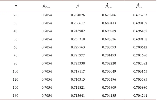
It can be observed that the Bayesian estimates of β are closer to the true value than the MLE of β_{, where the Bayesian estimate under the H-T loss}

function is slightly performing better even for a very small sample size of

20

n= _{. A graphical comparison of the true estimate of}β_{along with the}

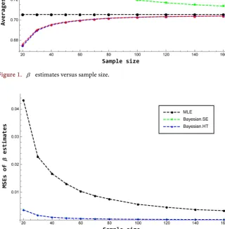
Bayesian estimates (under both S-E and H-T loss functions) and MLE as a function of sample size is given in Figure 1.

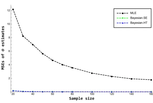
Figure 1 shows the the excellent performance of he Bayesian estimates compared to the MLE of the key parameter β_{. The Bayesian estimates tend to}

[image:11.595.246.499.72.377.2]

(12)

[image:12.595.210.533.76.302.2]

[image:12.595.210.531.185.512.2]

Figure 1. β estimates versus sample size.

Figure 2. MSE of β Bayesian estimates versus sample size.

Table 3. MSE for Bayesian estimates, under squared error and Higgin-Tsokos loss

functions, and MLEs of β.

θ MSE of βˆ MSE of βˆB SE. MSE of βˆB HT.

0.50000 0.01124360 0.0005077610 0.000507356 1.74410 0.01105730 0.0005163560 0.000516057 400000 0.01096100 0.0005190550 0.000518632

[image:12.595.211.539.584.650.2]

(13)

[image:13.595.210.541.102.313.2]

Table 4. Bayesian estimates, under squared error and Higgin-Tsokos loss functions, and

MLEs for the parameter β=0.7054 averaged over 10,000 repetitions.

n βFixed βˆ βˆB SE. βˆB HT.

20 0.7054 0.784026 0.673706 0.675263 30 0.7054 0.756617 0.689413 0.690189 40 0.7054 0.743982 0.695989 0.696467 50 0.7054 0.735310 0.698826 0.699158 60 0.7054 0.729563 0.700393 0.700642 70 0.7054 0.725977 0.701493 0.701690 80 0.7054 0.723338 0.702220 0.702382 100 0.7054 0.719117 0.703049 0.703165 120 0.7054 0.716315 0.703496 0.703585 140 0.7054 0.714821 0.703909 0.703980 160 0.7054 0.713641 0.704185 0.704244

Since the Bayesian estimates under both loss functions for β are superior to its MLE, Molinares and Tsokos [24] showed the improvement in the scale paramter (θ) when its estimate (10) is adjusted by using the Bayesian estimate of β instead of the corresponding MLE. Therefore, we calculated the adjusted estimate of θ using MLE and Bayesian estimates under S-E and H-T loss functions of β, shown in Table 5.

This proposed adjusted estimates,

θ

ˆB SE. and

θ

ˆB HT. , were averaged over the 10,000 repetitions. It can be appreciated that, based on the Bayesian influence on

β, θˆB SE. and

θ

ˆB HT. are better estimates than the MLE of θ (θˆ). This also can be seen in Figure 3, which visualize the performance of θˆB SE. and

θ

ˆB HT. compared to the corresponding MLE.

Figure 3 shows the excellent performance of the adjusted estimates of θ, where the adjusted estimate under the H-Twas slightly closer to the true value. The MSEs of these estimates of θ are displayed in Figure 4 given below.

The MSEs of the adjusted estimates of the shape parameter (θ ) are significantly smaller that the MSEs of the MLE estimate. The MSEs of the adjusted estimates are then displayed alone in Figure 5 to look closer at their performance.

It can be noticed that the adjusted estimate of θ under the influence of the Bayesian estimate with the H-T loss function, is better, particularly when considering small sample sizes.

We computed the adjusted estimate for the parameter θ and its MSE over 10000 repetitions for different values of θ and sample size n=40_{. The results}

are given in Table 6.

(14)

[image:14.595.223.524.100.481.2]

Figure 3. θ estimates versus sample size.

[image:14.595.221.522.285.487.2]

Figure 4. MSE of θ Bayesian and MLE estimates versus sample size.

[image:14.595.222.525.513.704.2]

(15)

[image:15.595.210.540.101.312.2]

Table 5. MLE Bayesian estimates, under squared error and Higgin-Tsokos loss functions,

and and MLEs for the parameter θ=1.7441 averaged over 10,000 repetitions.

n θ θˆMLE θˆB SE. θˆB HT.

20 1.7441 3.17139 1.3507 1.36422

30 1.7441 2.908 1.50142 1.5097

40 1.7441 2.73107 1.57545 1.58115 50 1.7441 2.59245 1.61556 1.61985 60 1.7441 2.48865 1.64065 1.64406 70 1.7441 2.41782 1.65803 1.66084 80 1.7441 2.36522 1.67055 1.67294 100 1.7441 2.26774 1.68719 1.68902 120 1.7441 2.20117 1.69776 1.69923 140 1.7441 2.15539 1.70537 1.70659 160 1.7441 2.11872 1.71089 1.71193

Table 6. MSE of θ estimates using Bayesian estimates, under squared error and

Higgin-Tsokos loss functions, and MLE of β.

θ θˆB SE. θˆB HT. MSE of θˆB SE. MSE of θˆB HT.

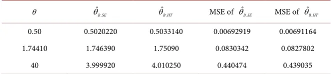
0.50 0.5020220 0.5033140 0.00692919 0.00691164 1.74410 1.746390 1.75090 0.0830342 0.0827802 40 3.999920 4.010250 0.440474 0.439035

The slight improvements in the estimation of the shape and scale parameters of the PLP is expected to jointly improve the estimate of the intensity function and therefore the reliability estimation of a software. For a fixed value of

1.7441

θ = and a sample size similar to the size of the collected data, n=40_,

the estimates of the intensity function VˆMLE

( )

t , VˆB SE.

( )

t , and VˆB HT.

( )

t were obtained when we use

β

ˆ,

β

ˆB SE. , and

β

ˆB HT. , respectively, in (2). That is,

( )

ˆ ˆ 1

ˆ _, _0, _0.

MLE t

V t t

β

β _θ

θ θ −  

′ = _{ } > >

  (36)

( )

. ˆ. 1 .

ˆ

ˆ B SE B SE _, _0, _0.

B SE t

V t t

β

β _θ

θ θ

−  

′ = _{ } > >

  (37)

( )

. ˆ. 1 .

ˆ

ˆ B HT B HT _, _0, _0.

B HT t

V t t

β

β _θ

θ θ

−  

′ = _{ } > >

  (38)

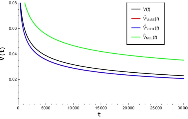
Their graphs (Figure 6) reveal the superior performance of VˆB SE′.

( )

t and

( )

.

ˆ_{B HT}

V′ t _.

In order to obtain Bayesian estimates of the intensity function, VˆB SE∗. and .

ˆ_{B HT}

V∗ _{, we substituted the Bayesian estimates of}_β_{and its corresponding}_θ

[image:15.595.208.539.357.431.2]

(16)

Figure 6. Graph for θ=1.7441 and the corresponding β _{Bayesian estimates and}

MLE’s used in VˆMLE′ , V′ˆB SE. , and VˆB HT′. (of time t) , n = 40.

( )

. ˆ. 1 .

ˆ

ˆ _, _0.

ˆ ˆ

B SE

B SE t

V t t

β β

θ θ

−

∗ ₌   _>

 

  (39)

( )

. ˆ. 1 .

ˆ

ˆ _, _0.

ˆ ˆ

B HT

B HT t

V t t

β β

θ θ

−

∗ ₌   _>

 

  (40)

The MLE of the intensity function, VˆMLE, is obtained using the MLEs of β

and θ. That is,

( )

ˆ ˆ 1

ˆ _, _0.

ˆ ˆ

MLE t

V t t

β β θ θ

−   = _{ } >

  (41)

The Bayesian MLE of the intensity function under the influence of the Bayesian estimates of β_{, denoted by}Vˆ_{B SE}_. and VˆB HT. , are obtained by substituting

β

ˆB HT. and

β

ˆB SE. with

θ

ˆB HT. and θˆB SE. , respectively, in (2):

( )

. ˆ ₁ . . . . ˆ

ˆ _, _0,

ˆ ˆ

B SE

B SE B SE

t

V t t

β

θ

−

 

= _ _ >

  (42)

and

( )

. ˆ 1 . . . . ˆ

ˆ _, _0.

ˆ ˆ

B HT

B HT B HT

t

V t t

β

θ

−

 

= _ _ >

  (43)

To measure the robustness of VˆB HT. with respect to VˆB SE. and VˆMLE, we

calculated the relative efficiency (RE) of the estimate VˆB HT. compared to the estimate VˆB SE. defined by:

(

)

( )

2 .

. . 2

.

ˆ _d

ˆ _,ˆ _.

ˆ _d

B HT B HT B SE

B SE

V t V t t

RE V V

V t V t t

∞ −∞ ∞ −∞  −    =  −   

∫

[image:16.595.211.532.72.276.2]

(17)

If RE=1_, Vˆ_{B HT}_. and VˆB SE. will be interpreted as equally efficient. If

1

RE< , VˆB HT. is more efficient than VˆB SE. . To the contrary, if RE>1, VˆB HT. is less efficient than VˆB SE. . Similarly, we compared VˆB HT. and VˆMLE. Bayesian

estimates and MLEs for the parameter β =0.7054 and θ =1.7441₍_{Table 7}_),

averaged over 10000 repetitions, are used, for n=40_{, to compare}Vˆ_{B HT}_. , VˆB SE. and VˆMLE using (44). The results are given in Table 8 and Table 9.

For the comparison of VˆB HT. and VˆB SE. , the RE V

(

ˆB HT. ,VˆB SE.

)

is less than 1, which implies that the intensity function using

β

ˆB HT. and

θ

ˆB HT. is more efficient than the intensity function under

β

ˆB SE. and

θ

ˆB SE. . Comparing VˆB HT. and VˆB SE. to VˆMLE, we obtained a similar result, establishing the superior

relative efficiency of Bayesian estimates over MLE estimates. The corresponding graphs for the intensity functions are given in Figure 7.

In addition, VˆB HT∗. and VˆB SE∗. are computed using Bayesian estimates for β and MLE estimates θ, which were less efficient compare to VˆMLE, VˆB SE. , and

.

ˆ_{B HT}

[image:17.595.233.516.329.464.2]

V . Based on the results, the Bayesian estimates under the H-T loss function will be used to analyze the real data.

[image:17.595.210.542.530.569.2]

Figure 7. Estimates of the intensity function (of time t) using values in Table 7, n = 40.

Table 7. Averages of the Bayesian (under the under squared error and Higgin-Tsokos

loss functions) and MLE estimates of β and θ.

β _βˆ

.

ˆ

B SE

β βˆB HT. θ θˆ θˆB SE. θˆB HT.

0.7054 0.743982 0.695989 0.696467 1.7441 2.73107 1.57545 1.58115

Table 8. Intensity functions with Bayesian and MLE estimates for β and θ.

( )

V t _Vˆ_MLE _Vˆ_{B SE}_. _Vˆ_{B HT}_.

0.2946

0.476465_⋅t− _0.352321_⋅_t−0.256018 _0.507238_⋅_t−0.304011 _0.5062_⋅_t−0.303533

Table 9. Relative efficiency of VˆB HT. to VˆMLE and VˆB BS. .

(

ˆB SE. ,ˆMLE

)

RE V V RE V

(

ˆB HT. ,VˆMLE

)

RE V

(

ˆB HT. ,VˆB SE.

)

(18)

3.2. Using Real Data

Using the reliability growth data from Table 1, we computed

β

ˆB HT. and the adjusted estimate

θ

ˆB HT. in order to obtain a Bayesian intensity function under H-T loss function. We followed Algorithm 2 to obtain the Bayesian intensity function for the given real data.

For the failure data of Crow, provided in Table 1,

β

ˆB HT. is approximately 0.501199 and

θ

ˆB HT. is approximately 2.07144. Therefore, with the use of

θ

ˆB HT. , the Bayesian MLE of the intensity function (VˆB HT.

( )

t ) for the data is given by:

( )

0.498801 .

ˆ_{B HT} _0.347933 _, _0.

V t ₌ _⋅t− t_> ₍₄₅₎

To obtain a Bayesian MLE for the reliability function under H-T loss function, we use this Bayesian estimate for the intensity function. The analytical form for the corresponding Bayesian reliability estimate, based on the data, is given by:

(

)

{

}

1

0.498801

. 1 1 1

ˆ _{| , ,} _{exp 0.347933} i _{d ,} _0.

i

t

B HT i i _t i i

R t t t x x t t

−

− = −

∫

> − >

(46)

Thus, the conditional reliability of the software given that the last two failure times were t39 =3181 and t40=3256.3 is approximately 63%.

(19)

3.3. Sensitivity Analysis: Prior and Loss Function

To answer the second research question, “Is the Bayesian estimate of the intensity function, V t

(

; ,

β θ

)

, of the PLP sensitive to the selections of the prior (both parametric and non-parametric priors) and loss function?”, we developed a simulation procedure, Algorithm 3, given below.

The algorithm compares the Bayesian and MLE estimates of the intensity function, V t

(

; ,

β θ

)

, under different prior PDFs, for various sample sizes, with the H-T and S-E loss functions. The relative efficiency is used to compare these estimates of the V t

(

; ,

β θ

)

. The relative efficiency with a value less than 1, larger than 1, and approximately equal to 1 indicate that the Bayesian estimates under the H-T loss function are more, less, equally efficient to the Bayesian estimate under the S-E loss function and the same analysis is applied when we compared to the MLE of V t

(

; ,

β θ

)

, respectively. The algorithm starts by initializing the shape and scale parameters of the PLP, β and θ , respectively, and the number of iterations p.

Algorithm 3. Simulation to compare Bayesian and MLE estimates of the intensity

(20)

For various sample sizes (n=20, 40,80,140_{), random failure times (time to}

failures) distributed according to the PLP are simulated using the initialized values of the PLP parameters. Then, the Bayesian and MLE estimates of the key parameter β are computed and used to compute the Bayesian estimates of θ, respectively. After a predetermined number of iterations, the average values of the Bayesian and MLE estimates of β and θ were used to obtain the analytical forms of the V t

(

; ,

β θ

)

under Bayesian, for both H-T and S-E loss functions and MLE, namely V VˆHT, ˆSE, and VˆMLE, respectively. Informative

parametric priors were considered such as the inverted gamma and the Burr PDFs, whereas the Jeffery prior was chosen as non-informative prior. In addition, probability kernel density function is selected as a non-parametric prior PDF. Probability kernel density estimation depends on the sample size, bandwidth, and the choice of the kernel function (K u

( )

). In this study, the optimal bandwidth (_h*_{) and kernel function were chosen to minimize the asymptotic} mean integrated squared error (AMISE). The simplified form of the AMISE is reduced to:

( )

(

)

( )

4 2

(

( )2

_{( )}

)

2

1 ˆ

AMISE

4 C K

f h k R f

n h

β = +_ ⋅ ⋅ ⋅ β _

⋅   (47)

where:

 C

( )

K =

_∫

(

K

( )

u

)

2du.

 n: sample size.

 _h: bandwidth.

 k₂ =

_∫

_−∞+∞u K u u2⋅

( )

d .



f

( )2

( )

β

_{is the second derivative of Burr PDF.} 

R f

(

( )2

( )

β

)

=

∫

(

f

( )2

( )

β

)

2

d

β

.



( )

_{( )}

( )

(

)

1 5

* 1 5

2 2 2

C K

h n

k R f β

−

 

 

= ⋅

 _⋅ 

 

.

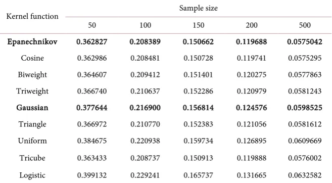
AMISE was numerically calculated using the optimal bandwidth, with respect to different samples sizes for each kernel function considered in this study, namely Epanechnikov, Cosine, Biweight, Triweight, Gaussian, Triangle, Uniform, Tricube, and Logistic kernel functions. The results is given by Table 10.

The minimum AMISE corresponds to the Epanechnikov kernel function

(

( )

(

2

)

1

3 1

4 u

K u = −u I ≤ ). In addition to the Epanechnikov kernel function, the

Gaussian kernel function (

( )

1 exp ₂2

2π R

u K u = _− _I

   ) was also used in the

calculation since it is commonly used for its analytical tractability.

Numerical integration techniques were used to compute the Bayesian estimates of the intensity function, V t

(

; ,

β θ

)

_{, parameters under both H-T and}

(21)

[image:21.595.210.539.103.284.2]

Table 10. Calculations of the AMISE with respect to different sample size, optimal

bandwidth, and kernel function.

Kernel function Sample size

50 100 150 200 500

Epanechnikov 0.362827 0.208389 0.150662 0.119688 0.0575042 Cosine 0.362986 0.208481 0.150728 0.119741 0.0575295 Biweight 0.364607 0.209412 0.151401 0.120275 0.0577863 Triweight 0.366740 0.210637 0.152286 0.120979 0.0581243 Gaussian 0.377644 0.216900 0.156814 0.124576 0.0598525 Triangle 0.366972 0.210770 0.152383 0.121056 0.0581612 Uniform 0.384675 0.220938 0.159734 0.126895 0.0609669 Tricube 0.363433 0.208737 0.150913 0.119888 0.0576002 Logistic 0.399132 0.229241 0.165737 0.131665 0.0632582

140 were generated where the parameters β and θ were initialized to be 0.7054 and 1.7441, respectively. In the analytical form (17), f1 and f2 are conditioned to be positive numbers and play a big role in assigning the weight of loss depending on the estimator’s behavior, whether underestimating or overestimating. Therefore, the simulation procedure was repeated three times according to the following cases:

1) f1> f2 2) f1< f2 3) f1= f2

The results for 1000 repetitions, f1> f2, and n=20, 40,80,140, are shown in Table 11.

It can be observed that the Bayesian estimate of the V t

(

; ,

β θ

)

_{under the H-T}

loss function (VˆHT) and S-E loss function (VˆSE) had an outstanding efficiency

compared to the MLE of the V t

(

; ,

β θ

)

₍Vˆ_MLE) for all sample sizes and prior PDFs, with the exception of the sample sizes 20 and 40 when inverted gamma PDF was the selected prior. The VˆHT was more efficient (6% - 11% estimation

improvement) compared to the VˆSE when Burr PDF is selected to be the prior.

The VˆHT had similar efficiency compared to the VˆSE when Jeffrey prior is

selected and for large sample sizes, whereas unsurprisingly VˆSE was more

efficient for small sample sizes since Jeffrey Bayesian estimate of the key parameter β tends to overestimate and for the H-T loss function gives more exponential weight on the extreme overestimate loss than the extreme underestimate loss when f1> f2. For Bayesian Gaussian and Epanechnikov kernel estimates, the VˆHT was more efficient compared to the VˆSE for sample sizes

20, 40

(22)

[image:22.595.212.538.129.489.2]

Table 11. The relative efficiency (RE) of the Bayesian estimate under H-T loss function,

ˆ_HT

V when f1>f2, compared to the Bayesian estimate under S-E loss function, VˆSE,

and the MLE, VˆMLE, of V t

(

; ,β θ

)

.

Prior PDF RE V V

(

ˆHT,ˆMLE

)

RE V V

(

ˆ ˆSE, MLE

)

RE V V

(

ˆ ˆHT, SE

)

Burr

20

n=

0.1356 0.1519 0.8923 Inverted gamma 4.2461 4.1632 1.0199

Jeffrey 0.0365 0.0289 1.2616

Gaussian kernel 0.1187 0.1346 0.8818 Epanechnikov kernel 0.1187 0.1346 0.8818

Burr

40

n=

0.3047 0.3345 0.9107 Inverted gamma 6.3934 6.2832 1.0175

Jeffrey 0.0166 0.0119 1.3947

Burr

80

n=

0.0136 0.0151 0.9007 Inverted gamma 0.8058 0.7934 1.0156

Jeffrey 0.0159 0.0144 1.1065

Burr

140

n=

0.0035 0.0037 0.9367 Inverted gamma 0.1421 0.1399 1.0155

Jeffrey 0.0040 0.0037 1.0680

The results for 1000 repetitions, f1> f2, and n=20, 40,80,140, are shown in Table 12.

Again, the Bayesian MLE estimate of the V t

(

; ,

β θ

)

under the H-T loss function (VˆHT) and S-E loss function (VˆSE) had an outstanding efficiency

(

; ,

β θ

)

(VˆMLE) for all sample sizes and prior

PDFs. When the inverted gamma was selected as prior, the VˆHT was more

efficient compared to the VˆSE for all sample sizes with an approximately 2% of

estimation improvement. As expected, the VˆHT was less efficient compared to

the VˆSE when Burr PDF, and Gaussian and Epanechnikov kernel densities are

selected as priors for sample sizes 20 and 40, since they tend to underestimate the V t

(

; ,

β θ

)

parameters, and the H-T loss function tends to put more weight on the extreme overestimation than on the extreme underestimation when

1 2

f > f _{. But the}Vˆ_HT and VˆSE had approximately similar efficiency for

(23)

[image:23.595.215.538.127.503.2]

ˆ_HT

V when f1< f2, compared to the Bayesian estimate under S-E loss function, VˆSE,

(

; ,β θ

)

.

Prior PDF RE V V

(

ˆHT,ˆMLE

)

RE V V

(

ˆ ˆSE, MLE

)

RE V V

(

ˆ ˆHT, SE

)

Burr

20

n=

0.2068 0.1860 1.1116 Inverted gamma 4.7351 4.8309 0.9802

Jeffrey 0.0232 0.0306 0.7589

Burr

40

n=

0.1500 0.1327 1.1305 Inverted gamma 5.9173 6.0152 0.9837

Jeffrey 0.0673 0.0785 0.8581

Burr

80

n=

0.0126 0.0121 1.0406 Inverted gamma 0.8155 0.8274 0.9856

Jeffrey 0.0326 0.0349 0.9365

Burr

140

n=

0.0180 0.0183 0.9814 Inverted gamma 0.2545 0.2576 0.9880

Jeffrey 0.0329 0.0338 0.9733

improvement) compared to the VˆSE when Burr Jeffrey is chosen to be the prior

PDF. The VˆHT had similar efficiency compared to the VˆSE for large sample

sizes and when Jeffrey prior is selected, whereas unsurprisingly VˆSE was more

efficient for small sample sizes since Jeffrey Bayesian estimate of the key parameter β tends to overestimate and for the H-T loss function gives more exponential weight on the extreme overestimate loss than the extreme underestimate loss when f1> f2. For Bayesian Gaussian and Epanechnikov kernel estimates, the VˆHT was more efficient compared to the VˆSE for sample sizes

20, 40

n= _{and 80 with 11% - 13% of estimation improvement even though they}

tend to underestimate and the H-T loss function puts more exponential weight on the extreme underestimation, but tend to have similar efficiency for sample size n=140.

(24)

[image:24.595.213.538.129.489.2]

ˆ_HT

V when f1=f2, compared to the Bayesian estimate under S-E loss function, VˆSE,

(

; ,β θ

)

.

Prior PDF RE V V

(

ˆHT,ˆMLE

)

RE V V

(

ˆ ˆSE, MLE

)

RE V V

(

ˆ ˆHT, SE

)

Burr

20

n=

0.0703 0.0702 1.0011 Inverted gamma 3.7132 3.7135 0.9999

Jeffrey 0.0612 0.0613 0.9981

Burr

40

n=

0.1195 0.1194 1.0008 Inverted gamma 7.3018 7.3022 0.9999

Jeffrey 0.1351 0.1352 0.9993

Burr

80

n=

0.0144 0.0144 1.0002 Inverted gamma 0.8626 0.8734 0.9876

Jeffrey 0.0250 0.0250 0.9998

Burr

140

n=

0.0065 0.0065 100000 Inverted gamma 0.1863 0.1863 100000

Jeffrey 0.0117 0.0117 0.9999

Again, the Bayesian MLE estimate of the V t

(

; ,

β θ

)

under the H-T loss function (VˆHT) and S-E loss function (VˆSE) had an outstanding efficiency

(

; ,

β θ

)

(VˆMLE) for all sample sizes and prior

PDFs, with the exception of the sample sizes 20 and 40 when inverted gamma PDF was the selected prior. It is observed that both VˆHT and VˆSE had similar

efficiency in estimation of the V t

(

; ,

β θ

)

_{for all sample sizes and priors}

considered in this study.

(25)

On the other hand, if the engineer does not have a prior knowledge of the key parameter β, it is still recommended to use H-T loss function in the Bayesian calculations with f1< f2.

Thus far, we showed the more accuracy in estimating a software reliability when applying the Bayesian analysis under the H-T loss function compared to the Bayesian analysis under the S-E loss function and the MLE of the subject analysis. The performed extensive analysis requires efficiency in utilizing the existing programming languages, which therefore requires some programming experience, we developed an interactive user interface application using Wolfram language to compute and visualize the Bayesian and maximum likelihood estimates of the intensity and reliability functions of the Power Law Process for a given data.

4. Conclusions

In the present study, we developed the analytical Bayesian estimates of the key parameter β, under Higgin-Tsokos and squared-error loss functions, in the intensity function where the underlying failure distribution is the Power Law Process, that is used for software reliability assessment, among others. The reliability function of the subject model is written analytically as a function of the intensity function.

The behavior of the key parameter β is characterized by the Burr type XII probability distribution. Real data and numerical simulation were used to illustrate not only the robustness of the squared-error loss function being challenged by the assumption of the Higgins-Tsokos loss function, but also the efficiency improvement in the estimation of the intensity function of PLP under Higgins-Tsokos loss function (VˆB HT.

( )

t ). For 100,000 samples of software failure times, based on Monte Carlo simulations and sample size of 40, the Bayesian estimate of β under Higgins-Tsokos loss function (

β

ˆB HT. ) performed slightly better than the Bayesian estimate of β under squared-error loss function (

β

ˆB SE. ) with respect to three different values of θ (0.5, 1.7441, 4). Even for different sample sizes (20, 30, 40, 50, 60, 70, 80, 100, 120, 140, and 160), similar results were achieved using β=0.7054_,θ =1.7441_{, and averaged over 10,000}

samples of software failure times.

As the MLE of the second parameter in the intensity function (θ) depends on the estimate of β, the adjusted estimate of θ

β

ˆ_{B HT}_. provided better performance compared to the adjusted estimate of θ using the βˆB SE.

( )

t . Moreover, the Relative Efficiency was used to compare the intensity function estimations, mainly using MLEs for both β_and θ (VˆMLE

( )

t ), using Bayesian estimate of β under the squared-error loss function and Bayesian of θ (VˆB SE.

( )

t ), and using Bayesian estimate of β under the Higgins-Tsokos loss function and Bayesian of θ (VˆB HT.

( )

t ), showing that VˆB HT.

( )

t is more efficient in estimating the intensity function V t

( )

with about 12% estimation improvement.

(26)

(

; ,

)

V t

β θ

, of the PLP sensitive to the selections of the prior, both parametric and non-parametric priors, and loss function? The parametric prior PDFs were Burr, Jeffrey, and inverted gamma probability distributions whereas the non- parametric priors were Gaussian and Epanechnikov kernel densities. The priors’ parameters were estimated using Crow failure times. Additionally, the optimal bandwidth and kernel functions were selected to minimize the asymptotic mean integrated squared error.

Using the developed algorithm, 1000 samples of software failure times with respect to four sample sizes of n (20, 40, 80, and 140) were generated from the PLP to compare the Bayesian estimates of V t

(

; ,

β θ

)

under the subject priors and loss functions using the Relative Efficiency among them. The simulation procedure was repeated three times for the cases when f1> f2, f1< f2, and

1 2

f = f _{. The results showed the efficacy of the Bayesian estimates of H-T loss}

function, and the choice of the f1 and f2 values depends on the prior knowledge of the key parameter β. It is recommended to choose values where

1 2

f > f _{when the engineer thinks the prior knowledge of}β is best characterized by Burr or Kernel based probability distributions with a proper justifi- cation, whereas a choice of f1< f2 and Jeffery’s prior is suggested when the engineer does not have a prior knowledge of β.

Thus, based on this aspect of our analysis, we can conclude that the Bayesian analysis approach under Higgins-Tsokos loss function not only as robust as the Bayesian analysis approach under squared error loss function but also performed better, where both are superior to the maximum likelihood approach in estimating the reliability function of the Power Law Process. The interactive user interface application can be used without any prior coding knowledge to compute and visualize the Bayesian and maximum likelihood estimates of the intensity and reliability functions of the Power Law Process for a given data.

Acknowledgements

We thank Majmaah University for funding the research, along with the support provided by the University of South Florida.

Conflicts of Interest

The authors declare no conflicts of interest regarding the publication of this pa-per.

References

[1] Duane, J.T. (1964) Learning Curve Approach to Reliability Monitoring. IEEE Transactions on Aerospace, 2, 563-566.https://doi.org/10.1109/TA.1964.4319640 [2] Crow, L.H. (1975) Tracking Reliability Growth. Proceedings of the 20th Conference

on Design of Experiments, Report 75-2, US Army Research Office, Research Trian-gle Park, NC, 741-754.