SDSS-IV MaNGA: The Spatial Distribution of Star
Formation and its Dependence on Mass, Structure and
Environment
Ashley Spindler
1
?
, David Wake
1
,
2
, Francesco Belfiore
3
, Matthew Bershady
4
,
Kevin Bundy
3
, Niv Drory
5
, Karen Masters
6
, Daniel Thomas
6
, Kyle Westfall
3
,
Vivienne Wild
7
1The Open University, Walton Hall, Milton Keynes, MK7 6AA, UK.
2Department of Physics, University of North Carolina Asheville, One University Heights, Asheville, NC 28804, USA.
3University of California Observatories - Lick Observatory, University of California Santa Cruz, 1156 High St., Santa Cruz, CA 95064, USA.
4Department of Astronomy, University of Wisconsin, 475 N. Charter St., Madison, WI 53706, USA.
5McDonald Observatory, University of Texas at Austin, 1 University Station, Austin, TX 78712-0259, USA.
6Institute of Cosmology and Gravitation, University of Portsmouth, Portsmouth, UK.
7School of Physics and Astronomy, University of St Andrews, North Haugh, St Andrews, KY16 9SS, UK.
Accepted XXX. Received YYY; in original form ZZZ
ABSTRACT
We study the spatially resolved star formation of 1494 galaxies in the SDSSIV-MaNGA Survey.
SFRs are calculated using a two-step process, using Hα in star forming regions and Dn4000 in
regions identified as AGN/LI(N)ER or lineless. The roles of secular and environmental quenching processes are investigated by studying the dependence of the radial profiles of specific star formation rate on stellar mass, galaxy structure and environment. We report on the existence of ‘Centrally Suppressed’ galaxies, which have suppressed SSFR in their cores compared to their disks. The profiles of centrally suppressed and unsuppressed galaxies are distibuted in a bimodal way. Galaxies with high stellar mass and core velocity dispersion are found to be much more likely to be centrally suppressed than low mass galaxies, and we show that this is related to morphology and the presence of AGN/LI(N)ER like emission. Centrally suppressed galaxies also display lower star formation at all radii compared to unsuppressed galaxies. The profiles of central and satellite galaxies are also compared, and we find that satellite galaxies experience lower specific star formation rates at all radii than central galaxies. This uniform suppression could be a signal of the stripping of hot halo gas in the process known as strangulation. We find that satellites are not more likely to be suppressed in their cores than centrals, indicating that the core suppression is an entirely internal process. We find no correlation between the local environment density and the profiles of star formation rate surface density.
Key words: galaxies: star formation – galaxies: evolution – galaxies: structure – galaxies: bulges – galaxies: groups: general – galaxies: clusters: general
1 INTRODUCTION
In the last two decades, large scale spectroscopic surveys
(such as SDSS, York et al. (2000), GAMA, Driver et al.
(2011) and zCOSMOS,Lilly et al.(2007)) have been a
driv-ing force in extragalactic astronomy. One of the principal results of these surveys is the characterisation of the bi-modality in galaxy populations across a variety of galaxy properties. Morphological type, colour, star formation rate,
? E-mail: ashley.spindler@open.ac.uk
stellar population age and gas content have all been shown
to be strongly bimodal (Baldry et al.(2006); Balogh et al.
(2004); Blanton et al. (2005, 2003); Baldry et al. (2004);
Blanton & Moustakas(2009);Peng et al.(2010a)). Broadly, galaxies can be split into two groups; star forming galax-ies which are typically low density, disk-like in shape and blue in colour, and quiescent galaxies, which are more com-pact than star forming galaxies, generally do not host spi-ral shapes and are red in colour. Quiescent galaxies also typically contain older stellar populations than star forming
Faber et al.(2007) found that while the number density of
blue galaxies has remained constant since z ∼1, the
num-ber density of red galaxies has increased. These observations suggest then that there are physical processes that move galaxies from the Star Forming type to the Quiescent type. In this work we explore the shut down of star formation, or ’quenching’ in local galaxies. We explore processes that shut down star formation at the local and global scale, and which act on different time scales.
In recent years, a new generation of integral field spec-troscopy (IFS) surveys have been employed to study the evo-lution of galaxies and by extension the process of quenching.
These IFS surveys (such as CALIFA,S´anchez et al.(2012),
MaNGA, Bundy et al. (2015), and SAMI, Bryant et al.
(2015)) use monolithic or multi-object spectrographs, and fibre optic bundles (or integral field units, IFUs) to observe galaxies both spatially and spectrally. The resulting data cubes provide spatially resolved information about the spec-tral make-up of the galaxy, allowing astronomers to study the spatial distribution of galaxy properties such as star for-mation, metallicity, kinematics and stellar age.
It has been suggested for some time that there are multiple channels by which galaxies can quench. Broadly speaking, there has been some consensus in the litera-ture to divide processes into two channels, those depen-dent on stellar mass and those that rely on
environ-ment (Silk 1977; Rees & Ostriker 1977; Peng et al. 2010b;
Mendel et al. 2013;Schawinski et al. 2014;Smethurst et al. 2015; Belfiore et al. 2016, 2017). Mass-quenching refers to the mechanisms that shut down star formation due to the intrinsic properties of the galaxy, such as radio-mode feed-back from AGN, morphological quenching, bar quenching
and halo-shock heating (Bower et al. 2006;Schawinski et al.
2007; Masters et al. 2011; Fabian 2012; Page et al. 2012; Heckman & Best 2014; Gavazzi et al. 2015; Belfiore et al. 2016,2017). Environmental-quenching refers to the mecha-nisms related to the extrinsic properties of a galaxy, these in-clude ram pressure stripping, tidal stripping, galaxy
harass-ment and strangulation (Gunn & Gott 1972; Abadi et al.
1999; Balogh et al. 2000; Lewis et al. 2002; Font et al. 2008; McCarthy et al. 2008; van den Bosch et al. 2008; Bialas et al. 2015;Peng et al. 2015;Gupta et al. 2017).
Interestingly however, it has been shown by some au-thors that mass and environment quenching may in fact
be part of the same mechanism. For exampleKnobel et al.
(2015) found that central galaxies in groups also respond to the environmental processes that are typically only associ-ated with satellites, they go on to suggest that the differ-ences in apparent mass dependdiffer-ences of satellite and central quenching occur because the properties that determine satel-lite quenching (e.g., dark matter halo mass, group centric distance, local overdensity) are independent of satellite
stel-lar mass. Carollo et al. (2016) and Smethurst et al.(2017)
both suggest that environmental processes work in tandem with mass and morphological quenching mechanisms in driv-ing the evolution of satellite galaxies in groups.
There are a number of physical processes which
act on galaxies in dense environments, which have
been widely studied in the literature. Ram
pres-sure stripping refers to the removal of gas from a galaxy due to super sonic heating in the
intraclus-ter medium (Gunn & Gott 1972; Cayatte et al. 1994;
Forman & Jones 1982;Markevitch et al. 2000;Solanes et al. 2001;Giovanelli & Haynes 1985;Cortese et al. 2011). Ram pressure stripping leads to a confinement of star formation to the centres of galaxies, as it predominantly acts on the outer
disk of later type galaxies (Koopmann & Kenney(2004b,a);
Cortese et al.(2012)). Similarly, galaxies may be subject to tidal harrassment from the surrounding dark matter halo and neighbouring galaxies, which affects star formation by removing gas from the disks or driving it into the galaxy
bulges (Hernquist 1989;Moreno et al. 2015).
If a galaxies outer halo of gas is stripped away, it will lose the ability to replenish the gas it uses in star formation, causing an eventual shut down in star formation often re-ferred to as starvation or strangulation (Larson et al. 1980; McCarthy et al. 2008;Peng et al. 2015). Interestingly, stran-gulation is predicted to have a different spatial pattern than gas stripping, occurring uniformly over the entire galaxy to produce anaemic spirals, as opposed to preferentially shut-ting down star formation in the disks or bulges of galaxies
(van den Bergh 1991;Elmegreen et al. 2002).
The existence of mass-based and secular quenching has been widely established in the literature, but the under-standing of the underlying physics on the other hand is not. Franx et al.(2008);Bell et al.(2012);Cheung et al.(2012); Pasquali et al. (2012); Wake et al. (2012) and Bluck et al. (2014) all point out the strong link between the presence of a large bulge and the likelihood that a galaxy will be
quenched.Martig et al.(2009) showed that the build up of a
spheroidal components from mergers or other processes can stabilise the gas in a galaxy against collapse and fragmen-tation. This prevents star formation and causes early type
galaxies to become red and dead. Smethurst et al. (2015)
found that quenching time-scales are correlated with galaxy morphology. Bars have also been linked to low the shut down of star formation in galaxies, both on a global scale and with the central few kpc of the galaxy core (Masters et al. 2011; Gavazzi et al. 2015)
The large bulges in quenched galaxies leads to the as-sumption that supermassive black holes may play a role in quenching, as the black hole mass is well correlated with bulge mass (Marconi & Hunt(2003);H¨aring & Rix(2004); McConnell & Ma(2013)). It has been show byFabian(2012) that radio-mode AGN are capable of inflating large bubbles of ionised gas, which could play an important role in regulat-ing star formation and gas accretion. However, no link has been found between the presence of a radiative mode AGN
and a suppression of star formation (Maiolino et al.(2012);
Cicone et al.(2014);Carniani et al.(2015)).
It appears then, from the mechanisms that drive mass based and environment based quenching, that they should provide opposing signals in galaxies. So-called “Inside-out” and “outside-in” quenching has been discussed in the
lit-erature (Tacchella et al. (2015); Li et al. (2015)). The
en-vironment channel may demonstrate an outside-in signal, whereby the cold gas is stripped from the outer disks or driven into the centre by tidal interactions, which would present enhanced star formation in the galaxy cores with re-spect to the outskirts. Mass quenching, if driven by AGN feedback or bulge growth, would instead demonstrate an inside-out quenching pattern, as the AGN quenches the star formation in the galaxy bulges first.
spec-troscopy surveys we can now study the effects of quench-ing at spatially resolved scales and identify the signals for both the mass based and environment based quenching
mechanisms. Belfiore et al. (2017) have already shown the
presence of inside-out quenching with their study of “cen-tral low ionisation emission region” (cLIER) galaxies, which they show could be green valley galaxies in the process of quenching. The outside-in process, instead, has been ob-served in MaNGA through stellar population analysis by Goddard et al. (2017b) who find slightly positive age gra-dients in early-type galaxies pointing towards outside-in progression of star formation. This pattern was found to
be independent of environmental density inGoddard et al.
(2017a) andZheng et al.(2017).Schaefer et al.(2017), used
the Sydney-AAO Multi-Object Integral Field Spectrograph (SAMI), to show that increasing local density correlated with reduced star formation in the outskirts of galaxies.
Conversely,Brough et al.(2013) found no evidence of
envi-ronmental quenching on a sample of galaxies studied using
theirHαprofiles, however this sample size was much smaller
thanSchaefer et al.(2017) with only 18 galaxies in the for-mer and 201 galaxies in the latter. Narrow band imaging of
Hα has been used to study the environmental dependence of
star formation in dense environments. In the Virgo cluster Koopmann & Kenney (2004b) showed that approximately half of their sample of 84 galaxies had truncated star forma-tion, and 10% had star formation rates which were uniformly suppressed. In the Calar Alto Legacy Integral Field Area
survey (CALIFA) P´erez et al. (2013) showed that massive
galaxies grew their mass inside-out by using stellar popula-tion spectral sysnthesis to find spatially and time resolved star formation histories.Gonz´alez Delgado et al.(2017) also studied spatially resolved star formation histories of a mor-phologically diverse sample of galaxies and found that galaxy formation happens very rapidly and in the past it was the central regions of early type galaxies where star formation
was at its most intense. In addition,Lin et al.(2017) found
evidence of bar induced star formation in the centres of so-called ‘turnover galaxies’, which exhibit a rejuvenated stellar populations in their cores.
In this paper we use a large sample of 1368 Star Forming and Composite AGN/Star Forming galaxies from the Fourth Sloan Digital Sky Survey Mapping Nearby Galaxies at
APO (SDSSIV-MaNGA,Bundy et al.(2015);Blanton et al.
(2017)) survey to study the spatial distribution of star for-mation and its dependence on stellar mass, core velocity dispersion, morphology and environment. We calculate star
formation rates using dust correctedHα measurements and
theDn4000spectral index and investigate the shapes of the
galaxy’s specific star formation rate profiles and investigate whether there is an inside-out or outside-in suppression of star formation with respect to galaxy’s internal and external properties.
This work is complemented by a parallel paper (Belfiore et al., submitted), which studies the sSFR profiles in the Green Valley and in central LIER galaxies.
This work is structured as follows. In Section2we
dis-cuss the MaNGA survey and our sample selection criteria.
In Section3we construct our star formation rates using dust
corrected Hα and show our model for using Dn4000 in
re-gions of the galaxies whereHαis unreliable. In Section4we show our results for the specific star formation rate profiles
−1.5 −1.0 −0.5 0.0 0.5 1.0 log10(N[II]/Hα)
−1.0
−0.5 0.0 0.5 1.0 1.5
log
10
(
O
[
I
I
I
]
/H
β
)
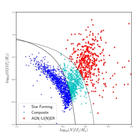
[image:3.595.309.526.110.332.2]Star Forming Composite AGN/LI(N)ER
Figure 1.The BPT Diagram for galaxies in the MaNGA survey. The positions of galaxies are calculated from the integrated flux over the entire IFU. Blue dots are the Star Forming Galaxies, cyan crosses and the composite galaxies and the red triangles are the AGN/LINER galaxies. The solid line is the relation from
Kauffmann et al.(2003) and the dashed line is fromKewley et al.
(2001).
and their dependence on a variety of galaxy properties, then
in Section5.1we split the galaxy sample in galaxies which
are centrally quenched or star forming. Finally we conclude
in Section7and discuss the roles of environment and mass
based quenching in relation to this work. We make use of a
standardΛCDM cosmology with Ωm =0.3, ΩΛ =0.7and
H0=70k m−1s−1M pc−1.
2 DATA
2.1 MaNGA Data
Mapping Nearby Galaxies at APO (Bundy et al. 2015; Law et al. 2015; Yan et al. 2016, MaNGA, ) is a multi-object IFU survey, one of the three projects under way as part of SDSS-IV (Blanton et al. 2017) using the 2.5-meter Sloan Foundation Telescope at the Apache Point Observa-tory (Gunn et al. 2006, APO, )). The goal of MaNGA is
to observe ∼10,000 galaxies using a range of IFU bundle
sizes (Drory et al. 2015). Observations began in 2014 and will conclude in 2020. The galaxy sample is chosen to include
galaxies with M∗ >109M and have a flat number density
distribution as a function of mass, while having no cuts in morphology, colour or environment. MaNGA has three main subsamples, the Primary, Secondary and Colour-Enhanced samples. The Primary sample makes up 50% of the target catalog, has a flat distribution in K-corrected i-band magni-tude and has a spatial coverage of1.5rewithin the IFUs. The Secondary sample contains 33% of the MaNGA sample, also
has a flat distribution inMi but instead selects IFUs which
sample makes up the remaining 17% of target galaxies, and
is selected to sample galaxies from regions in the NUV−i
versus Mi plane which are under sampled by the primary
sample such as low-mass red galaxies and high-mass blue galaxies.
We study galaxies from Data Release 14 (DR14). Using a range of IFU sizes most of the galaxies have full spec-tral coverage up to1.5half-light radii (re), though a subset are observed out to 2.5re. The IFU fibres are fed into the BOSS spectrograph, which has continuous coverage between
3600˚A and 10300˚A, with a spectral resolution of R ∼2000
(Smee et al. 2013; Drory et al. 2015). The MaNGA
obser-vations are reduced into data cubes by the Data Reduction
Pipeline (DRP,Law et al. (2016)) and then analysed using
the Data Analysis Pipeline (DAP, Westfall et al. in prep). The DAP fits the continuum, emission lines, kinematics and spectral indices from the DRP data cubes. Throughout this
paper we use the galaxy weights from Wake et al. (2017),
which are used to correct the sample from magnitude lim-ited to volume limlim-ited.
We make use of three of the products from the Data Analysis Pipeline (DAP, Westfall et al. in prep), the ALL binned data which combines the flux from all the spaxels in the data cube for maximum signal to noise, the VOR10
data which bins the spaxels into SNR>10 Voronoi bins and
the NONE binned data which includes all of the spaxels in the data cubes individually. The ALL binned data is used
when calculating our data cuts described in Section2.2. We
use the Voronoi binned data to calibrate ourDn4000-SSFR
model and the unbinned data is used in the final analysis. In addition we have rerun the DAP to produce a additional map of each galaxy which contains a single spatial bin out to0.125re, which is used to find the core velocity dispersion,
σ0, to match the definition used inSpindler & Wake(2017).
2.2 Sample Selection
DR14 contains 2791 galaxies across the primary, secondary, colour enhanced and ancillary samples. In this work we be-gin with the full MaNGA sample, with galaxies from the Primary, Secondary and Colour-Enhanced Samples.
We remove IFUs which contain two or more galaxies from the sample, which were identified by eye in the SDSS g-r-i imaging of the MaNGA galaxies, which cuts 153 fibre bundles from the sample. We do this to eliminate the need to calculate centres for both galaxies in order to find individual SFR profiles.
Throughout this work we wish to study galaxies which are dominated by different forms of ionising radiation, such as from star formation, Active Galactic Nuclei (AGN) and Low-Ionization (Nuclear) Emission Regions (LI(N)ER), or galaxies which are a composite of these emission types. As such, we measure the line intensities of Hα, Hβ, [N I I] (6585nm) and [OI I I] (5008nm) in the integrated fluxes of the DR14 data cubes and calculate the positions of these
galax-ies on the Baldwin-Phillips-Terlevich (BPT, Baldwin et al.
(1981)) diagram. We require that the emission line SNR in each of these lines be>2to accurately calculate their posi-tions on the BPT diagram, the limiting factors in the signal-to-noise are the strengths of theHβ and [OI I I] lines. We di-vide the galaxies into five groups: Star Forming for galaxies
which fall below theKauffmann et al.(2003) line,
Compos-ite for galaxies between the Kauffmann and Kewley et al.
(2001) lines, AGN/LI(N)ER for those above the Kewley
line, Low SNR AGN for galaxies with low SNR in theHβ
and[OI I I] lines but with integratedS N R>3inHαand [N I I] withlog10(Hα/N I I) >0.47 and finally Lineless galaxies for those galaxies with low SNR in all four diagnostic lines. We find 1049 Star Forming galaxies and 435 Composite galaxies which we examine in the main bulk of this paper, in addition there are 428 AGN/LI(N)ER and 22 low SNR AGN
galax-ies which we study in Section5.5, and 719 Lineless galaxies
which we discard from the sample. The BPT diagram for the
DR14 sample is shown in Figure1and shows the separations
used in this sample selection. Finally, we remove from the sample galaxies which have total Specific Star Formation
Rates (calculated using the model described in Section3) of
log10(SSF R)<−11.5.
The above classification are different to Belfiore et al. (submitted), in which we use a spatially resolved BPT clas-sifications. While the above work is interested in the roles of cLIER galaxies and their transition through the green valley, in this work we are interested in the much broader trends across the entire population. In this case we find that using the integrated flux to calculate the BPT class suits our needs, especially with the inclusion of the composite class which includes galaxies with star forming disks and AGN/LI(N)ER central regions which may be confused with only a SF-AGN/LI(N)ER cut. An alternative classification system in which we measured the BPT classification in the central 3” of each galaxy was tested, however we found that the majority of the galaxies which have different classes in this system were AGN/LI(N)ERs and lineless galaxies which are otherwise already removed from the sample due to low SSFRs.
A final cut is applied to the sample based on galaxy axis ratio. Edge-on disks with ab/a<0.3are removed from the sample, as we have found that their radial profiles are poorly resolved. A total of 128 galaxies are removed based on this cut. The final sample is then composed of 1494 galaxies, 1016 of which are star forming, 364 are composite and 114 are AGN/LI(N)ER.
In addition to the core MaNGA data products we make
use of the SDSS-MaNGA-Pipe3D (Pipe3D, S´anchez et al.
(2016b,a)) value added catalog. The Pipe3D data products were developed using the pipeline described inS´anchez et al.
(2016b) andS´anchez et al.(2016a) and applied to DR14. We
use the Single Stellar Population (SSP) cubes, which provide stellar mass surface density (log10(M)arcsec−2) maps of
the galaxies in DR14.
2.3 Other Catalogs
We make use of two additional catalogs in the analysis of
this work, the Yang Group Catalog (Yang et al.(2007,2008,
2009,2012)) and theBaldry et al.(2006) Environment Den-sity catalog.
Figure 2.Contours of the distribution ofDn4000and SSFR, the contours represent the1−,2−and 3−σ levels. The thick solid line is the mean fitted to the data we use for spaxels which are marked as composite or AGN/LINER from the BPT Diagram. Spaxels which we classify as low SNR are included in this model with an upper limit oflog10(S S F R)=−11.5. The dashed lines are
the standard deviation from the mean.
added to groups. From this catalog we use the Central and Satellite galaxy classifications, the dark matter halo masses and the group luminosities. The galaxy classifications and halo masses are based on rankings of the galaxies luminosi-ties.
There are a small number of galaxies in the MaNGA sample that are not in the SDSS DR7 (their NSA redshifts come from other sources) and so are not included in the Yang et al. catalog. We assign these galaxies central/satellite designations and group luminosities and halo masses by as-sociating them with Yang et al groups where possible. If a non-DR7 MaNGA galaxy has a projected separation within
r180of a group centre and a velocity within±1.5 times the
group velocity dispersion then we associate it with the group. If there is no matching group then the galaxy becomes its own group. The galaxy is then designated as either the group central or a group satellite depending on whether or not it’s r-band luminosity is the largest in the group. We then recal-culate the group luminosity including the new galaxy and calculate the other group properties following Yang et al. prescription.
Finally, we make use of the environment densities
around galaxies calculated in Baldry et al. (2006). These
densities are based on the distances to the 4th and 5th near-est neighbour galaxies withMr <−20(h=0.7). The density is calculated as log10(Σ) = 0.5∗log10(Σ4)+0.5∗log10(Σ5),
where ΣN = N/(pi ∗d2N) and dN is the distance to the
[image:5.595.44.280.103.256.2]Nth nearest neighbour. An important note here is that the matching between this catalog and the MaNGA data is not perfect, mainly owing to the redshift limits in the Baldry et al.(2006) galaxies.Baldry et al.(2006) is limited to 0.01 < z <0.085, which results in 15% of our MaNGA sample not being assigned environment densities. Due to the relationship between stellar mass and redshift in MaNGA (Wake et al. 2017), this means the galaxies without densi-ties are mainly at higher masses.
Figure 3.We show the star formation rates calculated using just the Hαmethod and just theDn4000method for star forming and composite galaxies in MaNGA. The dashed line shows the 1-to-1 relation and the solid line shows the linear regression fit. We provide the slope and intercept of the fit in the top left corner, with errors calculated from 1000 bootstrap resamplings of the data.
Figure 4.Values of the star formation rates calculated using the method described here for Star Forming (blue) and Composite (yellow) MaNGA galaxies, compared with their star formation rates calculated in Brinchmann 04 for the MPA/JHU catalog. The dotted line shows the one-to-one relations, the solid line is the linear fit to the star forming galaxies and the dashed line is the fit to the composite galaxies. The parameters of the fits are show in the top left corner, with errors calculated from 1000 bootstrap resamplings.
3 STAR FORMATION RATES
In this Section we will present our method for producing spatially resolved maps of star formation. We use a
two-source model, which calculates star formation rate fromHα
emission in the first instance in spaxels which are classified as star forming in the BPT diagram. These SFRs are used to model the dependence of specific star formation rate on the strength of the 4000 ˚A break (Dn4000). We then use this model to find the SFRs in spaxels with AGN and LINER contamination, and spaxels which are lineless, which would
otherwise be missed in a model which relies only on Hα
[image:5.595.307.541.365.523.2]form-−2.0 −1.5 −1.0 −0.5 0.0 0.5 1.0
log
10
(
S
F
R
,M
∗
/y
r
)
Central Galaxies Satellite Galaxies
9.0 9.5 10.0 10.5 11.0 11.5
log10(M∗/M) −12.0
−11.5 −11.0 −10.5 −10.0 −9.5
log
10
(
S
S
F
R
,y
r
−
1)
9.0 9.5 10.0 10.5 11.0 11.5 12.0
[image:6.595.46.500.86.426.2]log10(Lgroup, L)
Figure 5.We show the relationships between stellar mass in the left column, group luminosity in the right column, star formation rate in the top row and specific star formation rate in the bottom row, for galaxies with Star forming and Composite BPT types. Galaxies are coloured based on their environment, with centrals in red and satellites in blue. We include the mean values of SFR and SSFR at fixed M∗and Lgr o u pas solid lines for centrals and dashed lines for satellites. The dotted lines indicate the position of the sample cut in specific star formation rate atlog10(S S F R)=−11.5.
ing and composite galaxies to ensure the SSFR-Dn4000is as
representative of our sample as possible. This method is
in-spired by the work ofBrinchmann et al.(2004) (B04) in the
star formation estimations in the MPA/JHU DR7 catalog and allows us to include more galaxies than previous spa-tially resolved studies of star formation and study the star forming properties of galaxy bulges which would otherwise be removed due to contamination.
The final model will be applied to the DAP maps with no spatial binning, however it is important to begin with high signal-to-noise data so that we can detect very low
lev-els of Hα emission and therefore allow our Dn4000-SSFR
model to go to as low SSFRs as possible. As such we will begin our analysis using the Voronoi binned DAP products, which bins the spaxels into spatial regions which have a to-tal r-band signal-to-noise ratio per bin > 10. We apply an
additional cut to this data and only use bins with SNR >
20.
Following from our previous BPT-classifications and the
work ofBelfiore et al.(2016), we produce spatially resolved
BPT diagnostic maps from the Voronoi binned data and unbinned data. Bins and spaxels are placed into 4 cate-gories: Star Forming if they lie below the Kauffmann line, AGN/LI(N)ER if they lie above the Kauffmann line, lineless
if they have S N R<2in the Hα or NII lines and low SNR
AGN if the SNR forHβ orOI I Iis<2, the SNR for Hα and
N I I is>3, andlog10(N I I/Hα)>0.47.
The star forming bins from the Voronoi maps have their
star formation estimated using Hα, as detailed in Section
3.1, we then produce the model detailed in Section3.2using these SFRs. The unbinned maps are then treated in the same
way, with star forming spaxels using dust correctedHα to
estimate their SFRs and the AGN/LI(N)ER, low SNR and
lineless spaxels estimated using theDn4000model.
3.1 HαSFRs
The Hα flux relates the emission from excited hydrogen
clouds to the presence of high mass OB type stars, which
dominate the light emitted in young stellar populations.Hα
flux is readily absorbed and reprocessed by dust in the inter-stellar medium, we correct for this absorption by assuming
a foreground dust screen and using theCardelli et al.(1989)
extinction law:
LHα(Corrected)=LHα((LHα/LHβ)/2.8)2.36 (1)
T∼10,000K and corrects the deviation from the theoretical
ratio between the Hα and Hβ flux. The correctedHα flux
is converted into a SFR using the relation fromKennicutt
(1998), for aSalpeter(1955) IMF:
SF R(LHα)=LHα/1041.1 (2)
3.2 Dn4000SFRs
In areas of the galaxy where there is contamination in the
the Hα emission from AGN, LI(N)ER, old stellar
popula-tions and shocked gas we need a different estimator of Star Formation Rate. We also cannot simply ignore these por-tions of the galaxies, as the excess emissions often take place in important structures such as the bulge or bar. B04 showed
that there is a relation between SSFR and Dn4000, which
was used to estimate the SFRs of galaxies in DR4 and later DR7 of the Sloan Digital Sky Survey.
Using the Voronoi binned data we calculate the specific
star formation rates using Hα, in the regions which are
di-agnosed as star forming by the BPT diagram. As the star
forming bins only cover a range of Dn4000 values ranging
from 0.8 to 1.6 we also include the values of bins designated lineless, with a fixed upper limit SSFR oflog10(SSF R)=−12. We require that the bins used here have aS N R>20, to en-sure the quality of the model and to allow us to go to low
values of Hα. This approach is different from the one taken
in Belfiore at al. (submitted), where radial annuli containing no spectroscopically-classified star forming regions are dis-carded in computing radial profiles. This difference should be taken into account where directly comparing the radial sSFR profiles of these two works.
In Figure2we show theDn4000-SSFR relation, the
con-tours show the distribution ofDn4000and theHα predicted
SSFRs in the star forming bins, the solid line shows the mean SSFR at fixedDn4000and the dashed lines are the first stan-dard deviation from the mean. For galaxy regions which are marked as non-star forming, we assign a specific star
for-mation rate by interpolating theDn4000measurement with
the mean values from Figure 2. The SSFR decreases with
increasing Dn4000 and flattens out at high values once it
reaches the regime dominated by the lineless galaxies with highDn4000values. This flattening is artificial however, and is caused by the upper limit SSFR assigned to the lineless spaxels.
The value of the fixed SSFR limit applied at high
Dn4000values plays an important role in this work, as galax-ies with old stellar populations will be assigned this value. At a qualitative level, we treat this limit as zero star formation, galaxies with this SSFR at certain points are treated as sim-ply not forming stars whatsoever in those spaxels or radial bins. Quantitatively however, there is some dependence on the value of the limit on our work. For example, setting this value lower tolog10(SSF R)=−13has the effect of lowering total SSFRs of galaxies with −11.5<log10(SSF R) <−10.5
by 0.14 dex on average, in addition to exaggerating the ef-fects of any localised suppression of star formation within individual galaxies. However, we have tested using different values for the fixed SSFR limit and found that it has no effect on the conclusions of this paper.
To test the validity of this model, we compare the total
SFRs predicted in the star forming spaxels in each galaxy us-ingHαandDn4000in Figure3, with star forming galaxies in blue and composite galaxies in yellow. The two values of SFR agree very well, with most galaxies falling near the one to one relation with a scatter of 0.2 dex. Belowlog10(SF RHα)=−2
the agreement is not 1-to-1, however these galaxies all have
a very small number of spaxels (< 10) with both Hα and
Dn4000and so this can likely be attributed to the scatter
in the Dn4000 model. We perform an orthogonal distance
regression to fit a linear relation between the two values of star formation and find a very close to 1-to-1 fit, with a slope of0.91±0.08.
We compare the star formation rate in the MaNGA IFUs with the aperture corrected SFRs found in B04 for the
MPA/JHU catalog in Figure4. The B04 total star formation
rates are based using the broad band light from SDSS pho-tometry to correct the single fibre measurement to a global value. The scatter from the one-to-one line is fairly tight, with a standard deviation of 0.35 dex. We provide two lin-ear orthogonal distance regression fits to this comparison, one fit to the star forming galaxies and one to the compos-ite galaxies. The star forming galaxies are fit very well, with a slope of1.00±0.06, we find that galaxies with lower star for-mation in the MPA/JHU are generally given higher SFR in our work, this most likely due to the use of the aperture cor-rection to the 3” fibres in SDSS missing star formation which is present the MaNGA IFUs. For the composite galaxies we find the linear fit is worse than SF galaxies, but still close to 1-to-1 with a slope of0.86±0.18and a scatter of 0.5 dex.
As we will show in Section5.5, composite galaxies are more
likely to have suppressed star formations in their centres but still be forming stars in their disks, as the MPA/JHU values are based on the fibre readings at the centre of the galax-ies they would not pick up the extra star formation in the galaxy disk.
Throughout the rest of this paper we use the combina-tion ofHαandDn4000star formation rates for our analysis. We note that when the analysis is performed using just the
Dn4000predictions for star formation there is no qualitative difference on the conclusions presented here.
4 RESULTS
4.1 Global Properties
We begin by studying the global properties of galaxies in MaNGA. We calculate the integrated SFR, SSFR and Stel-lar Masses of star forming and composite galaxies from the IFUs using the ALL binned DAP MAPs, and plot their rela-tionships along with their group luminosities from the Yang
Catalogue in Figure5. We plot central galaxies from Yang
in red and satellites in blue and show the mean relations for those galaxies in each panel with solid and dashed lines, re-spectively. We include galaxies which fall below our sample cut in SSFR, which is shown by the straight dashed line in the top left and bottom panels.
In the top left panel of Figure5we show the M∗-SFR
−9
−10
−11
−12
log
10
(
S
S
F
R
)
N = 286.0
8.69< log(M∗)<9.97
r/r
eN = 314.0
Central Galaxies
9.97< log(M∗)<10.60
N = 336.0
10.60< log(M∗)<11.86
0.0 0.5 1.0 1.5 −9
−10
−11
−12
log
10
(
S
S
F
R
)
N = 127.0
0.0 0.5 1.0 1.5
r/r
eN = 111.0
Satellite Galaxies
0.0 0.5 1.0 1.5
[image:8.595.46.536.96.433.2]N = 90.0
Figure 6.The radial SSFR profiles in three bins of stellar mass. The individual profiles are shown by the cyan lines and the mean profile in the bin is shown by the solid red line. The dashed black line shows the mean profile of all galaxies in the sample. The number of galaxies in each bin is shown in the top left corner of each panel. The top row is the central galaxies and the bottom row is the satellite galaxies. The error bars are calculated from the scatter in 1000 bootstrap resamplings.
with upper limit SFR which would make up the ’red se-quence’ of quiescent galaxies, however as these are upper limits it is important to note that this region of the plot would appear more cloud like with accurate estimates of star formation. The mean SFRs of the centrals and satellites are shown, with the satellites having lower SFR at fixed mass than the centrals, with an overall difference in the means of
0.1±0.03dex. These results are echoed in the bottom left
panel, which shows the M∗-SSFR relation, with a difference
in the means of0.09±0.02dex. We again see that the satel-lites have lower SSFR than the central galaxies. There is a downward trend in the SSFR at fixed mass for both centrals and satellite galaxies.
In the top and bottom right panels of Figure5we show
the relationships of group luminosity with SFR and SSFR. For central galaxies these relationships are broadly similar to those with mass, as the luminosity of a group is tightly correlated with stellar mass for all but the most luminous groups. The satellite galaxies however are much more spread
out in the Lgr ou p-SFR plane, as low mass satellites with
low SFR can reside in very luminous groups, compared to centrals.
More massive star forming galaxies have lower specific star formation rates that low mass star forming galaxies, as
seen in Figure 5, and quenched galaxies are also typically
found at higher masses. This begs the question, what pro-cesses are taking place within more massive galaxies that are shutting down star formation. In the next sections we will study the mean radial profiles of specific star formation rates to investigate the mechanisms of star formation shut down, particularly whether the shut-down is inside-out or outside-in.
4.2 SSFR Profiles at fixed M∗
We wish to study the effects of internal and external pro-cesses on the distribution of star formation in galaxies within our sample. To test the effect of internal processes, we will investigate the mean profiles of galaxies in bins of stellar mass, core velocity dispersion and S´ersic index, and to test for external environmental effects we will compare central and satellite galaxies. To investigate the distribution of star formation we choose to study the radial profiles of the spe-cific star formation rates between0−1.5re. For each galaxy we separate the star formation maps calculated in Section 3into 15 bins of elliptical radius, each0.1re in width, from the centre of the galaxy. We calculate the mean SSFR of all the spaxels in each radius bin to find the radial profile of each galaxy.
r/r
e
−11.2−11.0 −10.8 −10.6 −10.4 −10.2 −10.0
log
10
(
S
S
F
R
)
8.69< log(M∗)<9.97, Cens: 286.0, Sats:127.0
9.97< log(M∗)<10.60, Cens:314.0, Sats: 111.0
10.60< log(M∗)<11.86, Cens:336.0, Sats: 90.0
0.0 0.5 1.0 1.5
r/r
e
−0.50 −0.25
0.00
0.25
0.50
(
S
S
F
R
sat−
S
S
F
R
cen)
/S
S
F
[image:9.595.94.485.105.633.2]R
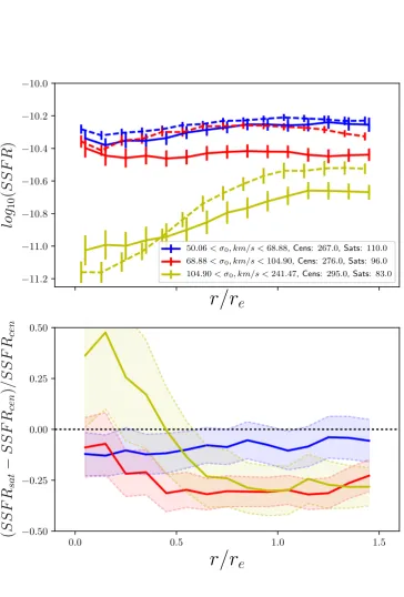
cenFigure 7.(Top) The mean radial SSFR profiles of central (dashed) and satellite (solid) lines in bins of stellar mass. (Bottom) The fractional difference between the central and satellite mean profiles in bins of stellar mass. The shaded regions and error bars represent the1−σ scatter in 1000 bootstrap resamplings.
be to integrate the light into elliptical radial bins, which can be done when processing datacubes with the DAP. We have tested this and found that it does not change the conclusions of this paper, so we choose to use the method described above.
We choose to calculate our radial profiles out to1.5reto ensure that the profiles are complete for each galaxy. While
it is possible to extend these profiles out beyond this point, particularly for galaxies in the Secondary MaNGA sample which are assigned an IFU to cover out to2.5reand for edge
on spirals which have radii going out to 5−6re, the vast
−2.0 −1.5 −1.0 −0.5 0.0 0.5 1.0 1.5 2.0
log
10[(
SSF R
r/re=0)
/
(
SSF R
Disk)] 050 100 150 200 250 300
No.
of
[image:10.595.44.259.71.263.2]Galaxies
Figure 8. Histogram showing the ratios between the SSFR in the centre most radial bin and the mean SSFR beyond r/re =
0.75. We show with a dashed line the cut between the centrally suppressed and unsuppressed galaxies, which marks where the disk has SSFR is approximately 10 times higher than the core of the galaxy.
and Dn4000 that 80% of galaxies are covered out to 1.5re and this number falls to 50% at 2.0re. Galaxies which are covered out to these larger radii tended to be assigned one of the larger IFUs and are preferentially from the Secondary galaxy sample, they are also typically more edge on disks.
In Figure 6 we plot the radial SSFR profiles of
cen-tral and satellite galaxies, in bins of stellar mass. The bins are chosen such that the total number of galaxies between centrals and satellites in each bin is constant. We show the individual profiles from0−1.5rein cyan, the mean profile of each bin in red, with errors calculated from 1000 bootstrap resamplings, and the mean profile of all galaxies in the sam-ple as a black dashed line in each panel to guide the eye and provide a point of reference.
In the lowest mass bin we see that the central and satel-lite profiles are largely flat, and while there are individual profiles that rise or fall with increasing radius the mean pro-files remain constant. In the medium mass bin the mean profile is still rather flat, but we see that the central mean profile has been pulled down slightly by a population of galaxies which have low central SSFRs, while the satellites remain flat. The differences in the centres of galaxies are sub-tle, and we explore this effect further in Section5.3. In the highest mass bin the galaxies with suppressed cores have significantly altered the shape of the mean profiles, which now exhibits a two-component shape with low SSFR in the centre and a flat profile outside of 1re.
We can see by comparing the mean profiles in each bin with the full sample mean that the total specific star for-mation rate drops as stellar mass increases and that the galaxies which have suppressed star formation in their cores
are mostly isolated to high masses. Figure6also displays a
bimodality, particularly at high masses, between two galaxy classes, those with relatively flat profiles and those which have suppressed star formation in their centres. However there is a difference regarding the extent of the suppression from the centre of the galaxy, with some galaxies beginning to show suppression at very small radii, and others at more intermediate radii.
We show the mean profiles for centrals and satellites
in the stellar mass bins in the same panel in Figure 7,
along with the fractional differences between these profiles. The satellite galaxies have lower SSFRs than the centrals
in all the stellar mass bins. In the low M∗ bin the
satel-lites have log10(SSF R) = −10.32±0.11 and the centrals
log10(SSF R) = −10.22±0.08. In the medium M∗ bin the
satellite SSFR islog10(SSF R)=−10.49±0.17compared to
log10(SSF R)=−10.39±0.14for the centrals. There is a large drop in both the satellites and centrals to the highM∗bin, to log10(SSF R)=−10.72±0.21andlog10(SSF R)=−10.68±0.20, respectively. In the lowest mass galaxies the satellites have lower SSFR at all radii than the centrals. In the medium mass bin the satellite have lower SSFR at all radii, but in the cores of the galaxies it appears that the satellites are not as suppressed as the centrals. In the highest mass bin, we see that the satellites have higher SSFRs in their cores and lower SSFRs at high radii. However due to the large vari-ance in the profiles caused by the separation of the galaxies which do and do not exhibit central suppression, it is diffi-cult to tell whether the differences seen in the cores of these galaxies are significant. As the central suppression appears to be strongly related to mass, the differences between cen-trals and satellites could be due to different stellar mass distributions within each bin, however we have checked the distributions and found that this is not the case.
We desire to determine a way to split galaxies between those that have flat profiles or are ‘Unsuppressed’ and those
that are ‘Centrally Suppressed’1. In Figure8we show the
ratio between the SSFR in the centre radial bin and the
mean SSFR beyond r/re = 0.75 (i.e. in the galaxy disk)
for the full galaxy sample. This figure shows that this ra-tio is bimodal, with most galaxies being evenly distributed around log10[SSF Rr/re=0/SSF Rdi sk] = 0, which represents
a flat profile, and a small population of galaxies around
log10[SSF Rr/re=0/SSF Rdi sk]=−1.25. We mark on this plot
with a dashed line the cut we make between centrally sup-pressed and unsupsup-pressed galaxies, where the SSFR in the disk is approximately 10 times the SSFR in the centre of the galaxy. We also define galaxies with a central SSFR of
log10(SSF R)<−11.5as centrally suppressed, because with-out this cut the lowest SSFR galaxies in the sample can be classified as unsuppressed.
The higher SSFRs in the centres of high mass satellites could be due to galaxies which have enhanced star formation in their cores, compared to their disks. This would counter-act the affect of the centrally suppressed galaxies lowering the mean SSFR, leading to a higher mean SSFR in satel-lites compared to centrals. We investigate this possibility in Section5.2.
4.3 SSFR Profiles at fixedσ0
In Spindler & Wake (2017), we showed that core velocity dispersion can be a more reliable tracer of environment
1 We choose to describe these galaxies as ‘Centrally Suppressed’
−9
−10
−11
−12
log
10
(
S
S
F
R
)
N = 267.0
50.06< σ0, km/s <68.88
r/r
eN = 276.0
Central Galaxies
68.88< σ0, km/s <104.90
N = 295.0
104.90< σ0, km/s <241.47
0.0 0.5 1.0 1.5 −9
−10
−11
−12
log
10
(
S
S
F
R
)
N = 110.0
0.0 0.5 1.0 1.5
r/r
eN = 96.0
Satellite Galaxies
0.0 0.5 1.0 1.5
[image:11.595.46.538.108.431.2]N = 83.0
Figure 9.The radial SSFR profiles in three bins ofσ0. The individual profiles are shown by the cyan lines and the mean profile in the
bin is shown by the solid red line. The dashed black line shows the mean profile of all galaxies in the sample. The number of galaxies in each bin is shown in the top left corner of each panel. The top row is the central galaxies and the bottom row is the satellite galaxies. The error bars are calculated from the scatter in 1000 bootstrap resamplings.
driven evolution of galaxies than stellar mass.σ0is invariant under environmental processes such as minor mergers and gas stripping, which lead to changes in the mass and size of galaxies. As such we repeat the analysis from the previ-ous section, but instead split galaxies by their core velocity dispersions.
We show the central and satellite profiles in Figure9,
using the same plot style as in the previous section. In the
lowestσ0 bin, we see that the mean profile for centrals and
satellites is relatively flat, there are a small number of cen-tral galaxies with suppressed cores, but no satellites. In the
mediumσ0bin the mean profile has a slight downward trend
and we once again see an increase in the number of galax-ies with suppressed cores, the satellites have a flat profile.
In the highestσ0 bin there are a large number of centrally
quenched galaxies which significantly affect the mean pro-files of both centrals and satellites, while the outer profile has remained flat.
We compare the mean profiles and fractional differ-ences between the mean satellite and central profiles in the
threeσ0 bins in Figure10. The satellite galaxies generally
have lower SSFRs than the centrals. The lowσ0 bins have
similar average SSFRs of log10(SSF R) =−10.30±0.11 and
log10(SSF R) =−10.25±0.08, for satellites and centrals
re-spectively. In the medium σ0 bin the satellite SSFR is 0.1
dex lower, at log10(SSF R) = −10.43±0.16 for the satel-lites compared tolog10(SSF R) =−10.30±0.12for the trals. There is a large drop in both the satellites and cen-trals to the highσ0 bin, tolog10(SSF R)=−10.82±0.24and
log10(SSF R)=−10.76±0.27, respectively. It appears thatσ0 is a better predictor for SSFR than stellar mass, which was
also found inWake et al.(2012).
In the low σ0 bin, the satellites have ∼ 10%less star
formation out tor/re=1.5, where the satellite profiles turn upward slightly and become more star forming than the
cen-trals. In the medium σ0 bin, we see that the satellites are
less star forming at all radii, however at low radii it ap-pears that the satellites exhibit less core suppression than the centrals as the fractional difference turns towards zero.
In the high σ0 bin the centrals have higher SSFRs at all
r/r
e
−11.2−11.0 −10.8 −10.6 −10.4 −10.2 −10.0
log
10
(
S
S
F
R
)
50.06< σ0, km/s <68.88, Cens: 267.0, Sats:110.0
68.88< σ0, km/s <104.90, Cens: 276.0, Sats:96.0
104.90< σ0, km/s <241.47, Cens: 295.0, Sats:83.0
0.0 0.5 1.0 1.5
r/r
e
−0.50 −0.25
0.00
0.25
0.50
(
S
S
F
R
sat−
S
S
F
R
cen)
/S
S
F
[image:12.595.93.458.90.629.2]R
cenFigure 10.(Top) The mean radial SSFR profiles of central (dashed) and satellite (solid) lines in bins ofσ0. (Bottom) The fractional
difference between the central and satellite mean profiles in bins ofσ0. The shaded regions and error bars represent the1−σscatter in
1000 bootstrap resamplings.
5 QUENCHING MECHANISMS
5.1 Centrally Suppressed Galaxies
As we have shown in the previous sections, the profile shapes seen in our sample are broadly bimodal. There are galaxies which have flat profiles, and those that have profiles which are centrally suppressed. We have also shown that in the
sec-tion we will explore the populasec-tions of centrally suppressed and unsuppressed galaxies separately.
To demonstrate this split, we plot the radial profiles
of the split populations in Figure 11. The non-suppressed
galaxies have predominantly flat profiles, however there is a subpopulation of galaxies which have enhanced SSFR in their cores and a falling profile. The centrally suppressed galaxies appear to be made of two groups, those with lin-ear rising profiles and those which have flat profiles in their outer regions that drop off sharply towards the central bulge. There are also a small number of galaxies which are centrally suppressed by our definition, but in fact exhibit some reju-venation in their cores.
In Figure12we show the fraction of central and
satel-lite galaxies which are centrally suppressed in bins of stellar mass. We find that there is no difference in the fraction of centrally suppressed galaxies at fixed mass between the cen-tral and satellite population. This figure implies then that the mechanisms behind the central suppression are indepen-dent from environment completely, and depend only on the galaxy’s internal properties. We also see a strong dependence on stellar mass for the fraction of suppressed galaxies, with essentially no galaxies at low mass exhibiting central sup-pression and 50% showing supsup-pression at high masses. This relationship holds when the fractions are instead calculated at fixedσ0.
One explanation for these centrally suppressed galaxies may be that we are simply tracing the existence of large bulges which formed a long time ago. This would manifest as mass profiles which increase dramatically in the centres of galaxies and SFR profiles which show a simple exponen-tial decrease. When the mass and SFR profiles are combined to produce the SSFR profiles, we would see the characteris-tic centrally suppressed galaxies. To test whether this is the case we show the SFR profiles for central and satellite
galax-ies in Figure13. This figure shows the increase in total SFR
with stellar mass we demonstrated in 5. We show the
un-suppressed and centrally un-suppressed galaxies with different
colour lines in Figure 13. There is a clear difference in the
SFR profiles of suppressed and unsuppressed galaxies, the centrally suppressed galaxies have lower SFR in their cores than their disks, and have lower SFR than the unsuppressed galaxies at all radii. This Figure shows that the differences in the SSFR profiles are not simply due to differences in mass distribution, but also reflect lower instantaneous star formation. The bimodality is not as strong in SSFR profiles,
which is due to the fixed SSFR limit in theDn4000model,
as the centrally suppressed galaxies have a ‘flat’ SSFR in their cores, the increasing mass profile causes the SFR pro-file to turn upwards, this artefact of the SSFR-Dn4000model masks the centrally suppressed galaxies slightly.
5.2 Comparison of Centrals and Satellite Profiles With the population split into centrally suppressed galaxies and unsuppressed galaxies, we can revisit the SSFR pro-files and determine the quenching effects operating on these different classes of galaxies. By studying the unsuppressed galaxies we can gain a better understanding of the processes which produce the reduction in SSFR at all radii in satel-lites compared to centrals. Studying the centrally suppressed
galaxies we can find if there is a difference in the amount of core suppression which happens in satellites and centrals.
In Figure14we show the mean profiles of galaxies, split
by whether they are centrally suppressed or not. Central galaxies are shown with solid lines and satellites with dashed lines, with the upper set of lines representing the unsup-pressed galaxies and the lower lines the supunsup-pressed galaxies.
We use the same mass binning scheme from Section 4.2.
Note that we do not include the profiles for low mass cen-trally suppressed galaxies, as there are too few galaxies in this bin to draw reliable conclusions. Firstly we can see that the centrally suppressed galaxies actually have reduce SS-FRs at all radii compared to the unsuppressed galaxies, not just in their cores. This is a crucial point, as it suggests that central suppression leads to external suppression, or at least that if fractional growth is low in the centre of galaxies it will be low in the outskirts. The low SSFRs in the out-skirts of suppressed galaxies is not a selection effect either, as the ratio we use to divide the sample would certainly al-low galaxies with SSFRs 2 or 3 dex higher in their disks, comparable to unsuppressed disks.
For the unsuppressed galaxies the low mass profiles are very similar to the profiles in the low mass bin for the full sample, due to there being very few centrally suppressed galaxies in this bin. The low mass satellites have a very flat profile, which has lower SSFR at all radii than the centrals in this bin, the central profile is also flat. In the medium mass bin the satellites appear to experience suppression at all radii compared to the centrals. In the high mass bin the satellites have higher SSFRs in their cores than the centrals,
but beyond∼0.5re their SSFR is consistently lower. This
could be due to high mass satellites that have had some star formation driven into their centres by tidal harassment or some other instability, as it appears that the satellite profile curves upwards, while the central profile curves down.
We see that for the centrally suppressed galaxies, in both the medium and high mass bin the profiles beyond
1.0reare quite shallow and rising, and that there is a sharp drop in SSFR towards the centres of the galaxies. The drop appears to happen at a larger radii for the satellite galaxies than the centrals, however both the centrals and satellites approach similar minimum SSFRs, due to the lower limit
imposed by our SSFR-Dn4000 model. We once again see
that there is a suppression of satellite star formation at all radii in the medium and high mass bins.
In Figure15we show the fractional differences between
the central and satellite galaxies in bins of mass, split by centrally suppressed and unsuppressed. The unsuppressed galaxies show a roughly uniform decrease in SSFR for satel-lites compared to centrals, except in the cores of high mass galaxies. For the centrally suppressed galaxies we also see a suppression at all radii in the satellites, though the SSFRs in the cores of the galaxies are approaching parity due to
the lower limits of our SSFR-Dn4000 model. This uniform
suppression of satellites could be a signature of
strangula-tion (van den Bergh(1991);Elmegreen et al.(2002)), which
we discuss further in Section5.3.
0.0 0.5 1.0 1.5
r/r
e−9
−10
−11
−12
log
10
(
S
S
F
R
)
Unsuppressed Galaxies
0.0 0.5 1.0 1.5
r/r
e [image:14.595.46.537.96.399.2]Centrally Suppressed Galaxies
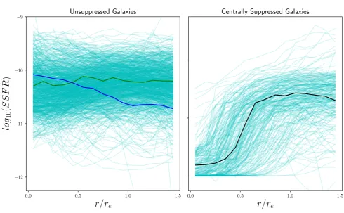
Figure 11.The radial SSFR profiles of galaxies in our sample which are centrally suppressed (left) and unsuppressed (right), as defined using the classification from Figure 8. In the two panels, we highlight ’typical’ profiles which fit the Centrally Suppressed (black), Unsuppressed (green) and Enhanced (blue) definitions.
Figure 12. We show the fraction of centrals (red) and satel-lites (blue) which are centrally suppressed, with respect to Stellar Mass.
that 183 galaxies are centrally enhanced using this classifi-cation, they are predominantly star forming galaxies, rather than composite. The fraction of enhanced galaxies decreases with stellar mass and satellites are more likely to be
en-hanced than centrals. At low mass18±8%of satellites are
enhanced, compared to14±5%of centrals, at high mass we
find that 14±3% of satellites have enhancement and only
6±1%of centrals do. We provide the fractional differences
between central and satellite profiles of centrally suppressed
and unsuppressed galaxies, with those that meet the
addi-tional enhanced criteria removed in Figure16. The fractional
differences for suppressed galaxies remain the same, however for the unsuppressed galaxies we see that the difference in the medium mass bin flattens and that the difference in the central radius bin of the high mass galaxies falls to zero. The exact causes of this enhancement is not clear, neither is the increased fraction in satellite galaxies. We briefly discuss
this in Section5.3, but would like to note that this will be
the subject of further study in a future work.
5.3 Environmental Quenching
Throughout this paper we have compared the profiles of central and satellite galaxies, as they largely reside in dif-ferent kinds of environments. At fixed mass, central galax-ies are found in lower density environments than satellites, since a satellite of equal mass would require a more mas-sive central to be present in the group. Satellites however are found in denser environments and are acted upon by a number of processes which can shut down star forma-tion, such as ram pressure stripping, tidal stripping and
strangulation (Gunn & Gott (1972); Abadi et al. (1999);
Balogh et al. (2000); Lewis et al. (2002); Kauffmann et al.
(2004); Koopmann & Kenney (2004a); McCarthy et al.
(2008); van den Bosch et al. (2008); Font et al. (2008);
Cortese et al. (2011); Bialas et al. (2015); Peng et al. (2015).
[image:14.595.46.278.462.624.2]−5.5 −4.5 −3.5 −2.5 −1.5 −0.5
log
10
(
S
F
R
)
8.69< log(M∗)<9.97
Unsuppressed Galaxies Centrally Suppressed Galaxies
r/r
eCentral Galaxies
9.97< log(M∗)<10.60 10.60< log(M∗)<11.86
0.0 0.5 1.0 1.5 −5.5
−4.5 −3.5 −2.5 −1.5 −0.5
log
10
(
S
F
R
)
0.0 0.5 1.0 1.5
r/r
eSatellite Galaxies
[image:15.595.46.539.105.434.2]0.0 0.5 1.0 1.5
Figure 13.The radial SFR profiles in three bins of stellar mass. We split galaxies based on their core suppression; centrally suppressed galaxies are shown in orange, with the solid blue lines indicating their means; the unsuppressed galaxies are shown in cyan with red lines for their means. The dashed black line shows the mean profile of all galaxies in the sample. The top row is the central galaxies and the bottom row is the satellite galaxies. The error bars are calculated from the scatter in 1000 bootstrap resamplings.
0.0 0.5 1.0 1.5
r/r
e −12.00−11.75 −11.50 −11.25 −11.00 −10.75 −10.50 −10.25 −10.00
log
10
(
S
S
F
R
)
8.69< log(M∗)<9.97
9.97< log(M∗)<10.60
10.60< log(M∗)<11.86
Figure 14.The mean SSFR profiles of centrally suppressed and unsuppressed galaxies. The upper set of lines are the unsuppressed galaxies, while the lower lines are the suppressed galaxies. Satel-lite profiles use solid lines and centrals use dashing lines. We do not include the low mass bin for the suppressed galaxies. We used the same three stellar mass bins as in Figure6.
star formation rates at large radii and a central
concen-tration of star formation (Koopmann & Kenney (2004a);
Cortese et al.(2011)). While we do see more satellites with
an enhanced central SSFR compared to centrals, we do not see and increase in suppression with radii as we might expect if ram pressure stripping were important. It could be that due to the cuts we made to effective radii in our sample to ensure good SNR we have excluded the regions of satellites which would be most affected by ram pressure stripping. The increased fraction of centrally enhanced galaxies in the satellite population could be a signal of tidal stripping and disruption, which has been shown to drive gas into the cen-tres of galaxies and cause an increase in circumnuclear star
formationHernquist(1989);Moreno et al.(2015).
Strangulation has been shown to be an effective method of quenching galaxies and it is theorised to pro-duce a uniform suppression across a galaxy’s radius, as opposed to concentrating star formation in the centre
or outskirts (Larson et al. (1980); van den Bergh (1991);
Elmegreen et al.(2002);McCarthy et al.(2008);Peng et al. (2015)). We do see a roughly uniform suppression of star for-mation in satellite galaxies at all radii for low and medium mass galaxies, especially when we remove the effect of cen-trally suppressed and enhanced galaxies from the sample, indicating that strangulation may be the dominant satellite
quenching mechanism. van den Bosch et al. (2008) argued
[image:15.595.44.277.509.657.2]r/r
e −0.50−0.25 0.00 0.25 0.50
( S S F Rsat − S S F Rcen ) /S S F Rcen
0.0 0.5 1.0 1.5
r/r
e −0.6−0.4 −0.2 0.0 0.2
[image:16.595.46.277.74.414.2]( S S F Rsat − S S F Rcen ) /S S F Rcen
Figure 15.(Top) The fractional differences between central and satellite galaxies in unsuppressed galaxies. We show the1−σ scat-ter from 1000 bootstrap resamplings as the shaded area. (Bottom) The fractional differences between central and satellite galaxies in centrally suppressed galaxies. We show the1−σscatter from 1000 bootstrap resamplings as the shaded area.
harassment which occur mainly at high dark matter halo mass. Satellites were found to be redder and more concen-trated than centrals, but these differences were independent of halo mass. Similar results were found using data from
the EAGLE cosmological simulations (Schaye et al.(2015))
byvan de Voort et al.(2017), who studied the gas accretion rates of simulated galaxies and found that satellites in dense environments are less able to replenish their cold gas than centrals, leading to a shut down of star formation. Finally, Peng et al.(2015) studied stellar metallicities and ages from local galaxies and concluded that strangulation, with an av-erage time-scale of 4 billion years, is the dominant mecha-nism behind galaxy quenching.
5.4 Morphological Quenching
Morphological quenching occurs when a dominant
spheroidal component is formed by mergers and other processes, which causes the gas within a galaxy to stabilise against fragmentation and star formation (Martig et al. (2009)). The build up of the bulge then may be what is causing the centrally suppressed galaxies, and may also explain why they have lower star formation rates in their outer regions than non-centrally suppressed galaxies. We now investigate the role of morphology in the suppression of
r/r
e −10.6−10.5 −10.4 −10.3 −10.2 −10.1
log 10 ( S S F R )
8.69< log(M∗)<9.97, Cens:237.0, Sats:97.0
9.97< log(M∗)<10.60, Cens:243.0, Sats:79.0
10.60< log(M∗)<11.86, Cens:150.0, Sats:34.0
0.0 0.5 1.0 1.5
r/r
e −0.50−0.25 0.00 0.25 0.50
[image:16.595.309.538.101.416.2]( S S F Rsat − S S F Rcen ) /S S F Rcen
Figure 16.(Top) The mean profiles for unsuppressed galaxies in bins of stellar mass, with the enhanced galaxy population re-moved. The error bars are calculated from the scatter in 1000 bootstrap resamplings and the stellar mass bins are the same as those from6. Note the different scale in the y-axis compared to Figure 14 (Bottom) The fractional differences between central and satellite galaxies in unsuppressed galaxies with centrally en-hanced galaxies removed. We show the1−σ scatter from 1000 bootstrap resamplings as the shaded area.
star formation by studying the profiles of galaxies at fixed
mass and r-band S´ersic index. If bulge like morphologies
do in fact play a role in quenching we would expect to see lower SSFRs at high S´ersic indices.
In Figure17we show the mean profiles for central and
satellite galaxies in bins of stellar mass and S´ersic index. The S´ersic index cuts are such that the lowest bin is mostly pure late type disk galaxies, the medium bin is likely made up of
disks with some bulges and bars, while the high S´ersic
in-dex bin is likely dominated by early-type galaxies with large bulges or elliptical morphologies. The shaded areas around
the lines represent the1−σscatter from the mean in 1000
bootstrap resamplings.
in-0.0 0.2 0.4 0.6 0.8 1.0 1.2 1.4 −11.2
−11.0 −10.8 −10.6 −10.4 −10.2 −10.0 −9.8 −9.6
log
10
(
S
S
F
R
)
8.69< log(M∗)<9.87
0.50<Sersic Index<1.38
1.38<Sersic Index<2.96
2.96<Sersic Index<6.00
0.0 0.2 0.4 0.6 0.8 1.0 1.2 1.4 r/re
Central Galaxies
9.87< log(M∗)<10.41
0.0 0.2 0.4 0.6 0.8 1.0 1.2 1.4 10.41< log(M∗)<11.00
0.0 0.2 0.4 0.6 0.8 1.0 1.2 1.4 −11.2
−11.0 −10.8 −10.6 −10.4 −10.2 −10.0 −9.8 −9.6
log
10
(
S
S
F
R
)
8.69< log(M∗)<9.87
0.50<Sersic Index<1.38
1.38<Sersic Index<2.96
2.96<Sersic Index<6.00
0.0 0.2 0.4 0.6 0.8 1.0 1.2 1.4 r/re
Satellite Galaxies
9.87< log(M∗)<10.41
[image:17.595.44.541.106.432.2]0.0 0.2 0.4 0.6 0.8 1.0 1.2 1.4 10.41< log(M∗)<11.00
Figure 17.The radial SSFR profiles for central galaxies (top) and satellite galaxies (bottom), in bins of stellar mass and S´ersic Index. In each bin the blue line represents low S´ersic index galaxies, red is medium and yellow is high S´ersic index. The shaded areas represent in the1−σscatter from the mean in 1000 bootstrap resamplings.
dex strongly affects the normalisation of the profile. Higher S´ersic index galaxies, i.e. those that are more dominated by bulge-like morphologies, have lower SSFRs across their en-tire profiles.
For the satellite galaxies, many of the properties are the
same as the centrals. The low and medium S´ersic index
pro-files agree well at low and medium masses, but the medium S´ersic index galaxies have slightly lower SSFRs at high mass in their disks. The high S´ersic index satellites have very dif-ferent profiles compared to the centrals however. We see that the cores of these satellite galaxies are enhanced compared to the general population in both the low and medium mass bins. There also appears to be some enhancement compared
to high S´ersic index centrals in the high mass bin, but not
to the same extent as the other profiles. This enhancement may be due to gas being driven into their centres of galaxies by tidal interactions, however it is unclear why this would mainly affect galaxies with high S´ersic indices.
We also investigate the profiles in bins of stellar mass
and σ0 simultaneously. We show the mean profiles for
cen-tral and satellites galaxies in Figure18, with galaxies split
by mass in the columns and into three bins of σ0 in each
panel, we omit the low mass-high σ0 profile, as there are
< 3 galaxies in this bin. Velocity dispersion has
previ-ously been found to be a better predictor of galaxy colour, bulge mass, bar strength and whether a galaxy is passive or
notDas et al.(2008);Wake et al.(2012);Teimoorinia et al.
(2016);Spindler & Wake(2017). Once again we see that as
stellar mass increases the galaxies become more centrally suppressed, in addition we see that in the high mass bins
the galaxies with the highestσ0 exhibit the strongest
sup-pression of star formation. This supsup-pression occurs both in the cores of these galaxies, but also in the SSFR at all radii. This is particularly strong for central galaxies, where the high mass galaxies with low or medium dispersions are not significantly suppressed compared to the full sample mean and the high dispersion galaxies are very suppressed. One possible explanation for enhancement of high S´ersic satellites is that it is a selection effect. If these galaxies have very high star formation rates in their centres the light could wash out the disk when the single component fit is attempted, making them seem more bulge dominated.
Combining the results from Figures17and18, we see a