Technical efficiency and total factor productivity in Czech agriculture

czech agriculture experienced a couple of insti-tutional and economic changes in the last two dec-ades. The most important one is the accession to the European Union and the accompanying implemen-tation of the cAP principles. These changes had a significant influence on the performance, structure and size of czech agriculture. With regard to this, an important question arises: are czech farmers taking advantage of the opportunities of the cAP and the common market or are they falling behind? This paper shows the development of the performance of czech agriculture and its branches, and identi-fies the factors which determine the successes and failures of the growth of czech agriculture since the EU accession. in particular, the paper focuses on the development of technical efficiency and the total factor productivity (TFP) and their components in the period 2004–2007.

The following questions will be elaborated. The first relates to the technical change and technical efficiency. The aim is to identify whether agricul-ture is following a path of sustainable development, characterized by the adoption of innovation and the reduced waste of resource due to the inefficient input use. The second concerns productivity development. The aim is to identify the key factors which determine

the productivity development in czech agriculture. The last question concerns the sector-specific devel-opment. The aim is to assess whether the branches are determined by the same factors or whether idi-osyncratic developments have occurred.

These questions will be elaborated by estimating a joint stochastic frontier production function model for czech agriculture. Then, the estimates are used to construct the TFP. Furthermore, the TFP and techni-cal efficiency are broken down into their individual components.

Technical efficiency in czech agriculture has been analyzed by several authors, e.g., hughes (1999), Mathijs et al. (1999a, b, 2001), curtiss (2002), Juřica et al. (2004), Jelínek (2006), Medonos (2006) and Čechura (2009, 2010). We complement these studies with an analysis of technical efficiency and the TFP development, as well as their determining factors, since the czech republic accession to the EU.

MATERIAL AND METHODS

The estimation of a stochastic frontier production function model for czech agriculture follows Čechura (2010). Čechura (2010) showed that the presence of

Technical efficiency and total factor productivity

in Czech agriculture

Lukáš Čechura

Department of Economics, Faculty of Economics and Management,

Czech University of Life Sciences Prague, Prague, Czech Republic

Abstract: The paper deals with the analysis of technical efficiency and the total factor productivity (TFP) in czech

agri-culture. The aim is to identify the key factors determining the efficiency of input use and the TFP development. The Fixed Management model is used for the estimation of technical efficiency and the construction of TFP for the total agriculture and its individual branches. The results show that technical inefficiency is an important phenomenon in czech agriculture and its individual branches. The TFP development is determined by all components, i.e., technical efficiency, scale effect, technological change and management. Their contributions differ intrasectorally and intersectorally, and also in time. Fi-nally, the developments in the individual branches are characterized by idiosyncratic factors, as well as the systemic effect, especially in the animal production. The most important factors which determine both technical efficiency and TFP are the factors connected with institutional and economic changes, in particular a dramatic increase in the imports of meat and increasing subsidies.

Key words: technical efficiency, technology, heterogeneity, total factor productivity (TFP), Fixed Management model and

agriculture

a significant firm heterogeneity overestimates the technical inefficiency. considering both the theoreti-cal criteria of the production function and significant firm heterogeneity, the author suggests using the Fixed Management model for the measurement and analysis of technical efficiency. This paper will use the same data set, and therefore the Fixed Management model, in the analysis of technical efficiency; the total factor productivity development is considered to be a proper choice. That is, we will re-estimate the Fixed Management model and will use it in the

construction of TFP (see also Čechura 2009)1_.

The analysis is based on the assumption that the production possibilities can be approximated by a frontier production function which has the translog form (as in Čechura 2010). The details of the fitted Fixed Management model are provided in the fol-lowing section, followed by the information about the construction of TFP.

Fixed Management model

Álvarez et al. (2003 and 2004) specified the Fixed Management model as a special case of the random Parameters model in the following form:



, , ;



ln



, , ;



0 ln

ln  _{x β}  _x  _β 

i it i

it

it f t m f t m

TE

lnTE_it = – u_it (1)

and





          it it i it it it it

it y v u f t m v u

y ln lnα ln ,x , ;β

ln 0

  mmi  mmmi 



t tmmi



t ttt 



x xtt xmmi



it it itvituit

 



 _{x x B x}

xxln ´ ln 2 1 ´ln β β β β 2 1 β β β 2 1 β

α 2 2

0



t tm i



tt



x xt xm i



it it it it it i

mm i

mm  m   m t t   t m  v u



     _{x x B x}

xxln ´ ln 2 1 ´ln β β β β 2 1 β β β 2 1 β

α 2 2

0 (2)

where x_it is a vector of inputs containing K = 4

pro-duction factors – Labour (A_it), capital (C_it), Land

(L_it) and Material (M_it). indices i, where i = 1, 2,…, N,

and t, where t

 

i , refer to a particular agricultural

company and time, respectively, and 

 

i

repre-sents a subset of years T_i from the whole set of years

T (1, 2,…,T), for which the observations of the i-th

ag-ricultural company are in the data set (see unbalanced

panel). α is an intercept (productivity parameter). β

are parameters to be estimated that determine the

production function f. Technical efficiency, TE_i(t),

with 0 ≤ TE_i(t) ≤ 1, captures the deviations from the

maximum achievable output. v_it is the random

er-ror and u_i(t) is the inefficiency term. The random

error (statistical noise) v_it and the technical

ineffi-ciency term u_i(t) of the stochastic frontier production

function model are assumed to be ~ (0,σ2)

v it iid N

v , ) σ , 0 ( ~ 2 )

(t u

i iid N

u 

and to be distributed independently of each other, and of the regressors (for further

refer-ences see Kumbhakar and Lovell 2000). ~

 

0,1

i

m

represents the unobservable fixed management. The

symbol

•

expresses that 

i

m could possess any

distribu-tion with zero mean and unit variance (see hockmann

and Pieniadz 2008). The difference between the real (m_i)

and optimal ( 

i

m ) management determines the level

of technical efficiency /see relation (1)/. Technical efficiency is defined by:

it t

it t

TE γ γ γx´lnx

ln  0  (3)

where



2 2



0

2 1 ) (

γ _{ }  _{  }  i i mm i

i

m m m m m

_{ }



_ 



i i tm

t m m

γxβxm



mimi



Thus, the technical efficiency consists of three components:

(i) time-invariant, firm specific effect –

manage-ment – γ₀,

(ii) interaction of m* _{with time – technological change}

– γ_t,

(iii) interaction of m* _{with the inputs quantity and}

quality – scale effect – γ_x.

Álvarez et al. (2004) showed that u_it can be

esti-mated, according to Jondrow et al. (1982), as (4) with

simulated mi according to relation (5).













 

 





 

                 σ λ ε λ/σ ε Φ λ/σ ε φ λ 1 λ σ , ε 2 i it i it i it i it it m m m m u

E (4)

where v u     _, v u   

 and itvituit











y X δ



δ X y δ X y , , , ˆ 1 , , , ˆ 1 , , ˆ 1

1 , ,

i i i R r R

r ir i ir i i i i m t f R m t f m R m E      





 ₍₅₎

The Fixed Management model is fitted with a maxi-mum simulated likelihood in the computer program nLogiT version 4.0 – LiMDEP version 9.0 (green 2007). in the model, all variables are divided by their

geometric mean. That is, fitted coefficients represent the production elasticities evaluated on the geometric mean of a particular variable.

Total factor productivity

The total factor productivity is calculated in the form of the Törnqvist-Theil index (TTi) (see, e.g., Čechura and hockmann 2010). The Törnqvist-Theil index exactly determines the changes in production resulting from input adjustments having a production function the translog form (for the proof see Diewert 1976). Furthermore, caves et al. (1982) show the TTi extension for the multilateral consistent comparisons. The index is constructed as the deviation from the sample means. The input index for the variable return to scale (VrS), or the constant return to scale (crS), respectively, is given by:







      _{ }       _   K

j itj j itj j j j itj itj VRS

it x x x x

1 ____ __________ , , ______ ______ ,

, ε ln ln ε ln ε ln

ε

2 1

ln _{0 0}







      _{ }       _   K

j itj j itj j j j itj itj VRS

it x x x x

1 ____ __________ , , ______ ______ ,

, ε ln ln ε ln ε ln

ε

2 1

ln _{0 0}

with





j it j it j it x t f , , , _ln ; , ln

with 0 x

β 

 

 ₍₆₎

resp.

∑

∑

∑

∑

∑

= = = = =             − +       ₋             + = K

j K itj

i itj j it j K i j j j j it K i j j K

i itj j it CRS

it x x x x

1 __________ __________ , 1 , , ______ 1 ______ , 1 1 , , _ln ε ε ln ε ε ln ln ε ε ε ε 2 1 ln 0 0 0 0 0 0 ι

∑

∑

∑

∑

∑

= = = = =             − +       ₋             + = K

j K itj

i itj j it j K i j j j j it K i j j K

i itj j it CRS

it x x x x

1 __________ __________ , 1 , , ______ 1 ______ , 1 1 , , _ln ε ε ln ε ε ln ln ε ε ε ε 2 1 ln 0 0 0 0 0 0

ι (7)

A bar over a variable specifies the arithmetic mean over all observations. if no aggregation is needed, i.e., only the development of one variable is depicted, the index simplifies into the deviation from the mean of the variables. That is, the output index and efficiency index are:

______

ln ln

lnit yit yit and

______

ln ln

lnit TEit TEit (8)

Since TFP is a combination of scale effect, technical efficiency effect, technological change effect and man-agement effect, the required indices are defined:



 



t t t t tt tt



it     

 2 1 ln

with





t m t x f itj i

t _

 

 ln , , , (9)











m m i i m i m i



it 1₂ ε ε m m ε m ε m

μ

ln  ₀   

with





i i j it m _m m t x f   

 ln , , ,

(10)

Using these definitions, TFP and its breakdown is given by:

MAN TCH TE SE

TFPitlnitlnCRSit lnitlnitlnitlnit

ln

with CRS

it VRS it it   

 ln ln

ln (11)

changes in TFP can be expressed either as a ratio (on the mean) of the output and input index (for crS) or as a multiplication of the TFP components, i.e., scale effect (SE), technical efficiency effect (TE), technological change effect (Tch) and management effect (MAn).

Data set

Since the same panel data set is used in Čechura (2010), the data description provides only basic

in-formation.2 _{The panel data set is drawn from the}

database of the creditinfo Firms’ Monitor, collected by the creditinfo czech republic, s.r.o. The database contains all registered companies and organisations in the czech republic.

Since the creditinfo database does not contain information about the quantity of land employed in the production of a particular agricultural company, the database LPiS is used for the input factor Land. Price indices and the regional wages are drawn from the czech Statistical office. The source of the official land prices is a study by němec et al. (2006).

The analysis uses information from the final ac-counts of the companies whose main activity is agri-culture, according to the oKEČ classification (oKEČ 01). Therefore, the analysis concerns agricultural companies, i.e., corporations. Since not all informa-tion can be found for all agricultural companies in the database, only those companies having two or more final accounts in the database over the period 2004–2007 are used; non-zero and positive values are used for the variable of interest. in addition, outliers were removed. After the cleaning process,

the unbalanced panel data set contains 1004 agricul-tural companies with 3103 observations, covering the period from 2004 to 2007, i.e., 3.09 observations per company in average.

The following variables, as defined above, are used in the analysis: output, Labour, Land, capital and Material. output is represented by the total sales of goods, products and services of the agricultural company. output was deflated by the index of agri-cultural prices (2005 = 100). The Labour input is the total personnel costs per company, divided by the average annual regional wage in agriculture (region = nUTS 3). The total quantity of land employed in the production process of a particular agricultural company is adjusted by the land quality. Land quality is expressed as the ratio of the official land price of

the j-th region to the maximal official regional land

price. That is, the total quantity of land employed

in the production process of the i-th company was

multiplied by the quality index of the region to which the company belongs. capital is represented by the book value of tangible assets and it is deflated by the index of processing (industry) prices (2005 = 100). Finally, the Material variable is used in the form of the total costs of material and energy consumption per company, and it is deflated by the index of

pro-cessing prices (2005 = 100).3

The development indicators show (see Čechura 2010) that the average growth rate of the output as well as all inputs is negative in the data set. Despite this, labour productivity, land productivity, land in-tensity and capital inin-tensity in the sample increased in the period from 2004 to 2007. This suggests that agricultural companies are subject to substantial adjustment processes regarding the structure of pro-duction factors.

RESULTS

Parameter estimates

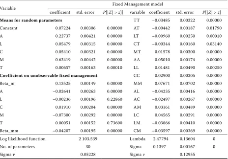
First, the results of parameter estimates are dis-cussed. The estimated production elasticities (Table 1) satisfy the criterion of both monotonicity and quasi-concavity, i.e., the elasticities are positive and the diminishing marginal productivity for each input

was estimated (_{ }2_{ }0

r r

rr , for r = A, L, C and

M). That is, the estimates are consistent with the

economic theory (at least on the sample mean).

Production elasticities were also found to be robust under different model specifications (see Čechura 2010). Material has the highest impact on production,

with production elasticities (β_M) 0.63419, which is also

consistent with the empirical observations. Labour

elasticity (β_A) is 0.227, which corresponds to the ratio

of personnel costs to the total output. The production elasticity of Land is at the same level as the elasticity of capital. however, capital determines production with a lower intensity than we would expect. This might be caused by two factors that work together. Since we are working with accounting data, the vari-able capital does not contain the information about leasing. however, leasing is an important source of capital in czech agriculture. its role is reinforced by the imperfections in the czech capital market.

Technical change has a positive impact on pro-duction; however, it decelerates over time. The hypothesis that the parameters are time-invariant

(h₀:  β_T = β_TT = β_AT = β_LT = β_CT = β_MT = 0)4 _was

rejected at a 5% level of significance. Moreover, the null hypothesis about the hicks neutral technological

change (h₀: β_AT = β_LT = β_CT = β_MT = 0)5 _{was rejected}

as well. The technological progress was Material us-ing and Labour, Land and capital savus-ing.

Furthermore, the z-test and Lr test reject the null

hypothesis about the statistical insignificance of the parameter lambda (Lr = 1941.66; critical value

71 . 2 ) 1 (

´mixed´ 2

025 , 0

1 

_{ ). Thus, the value of the}

pa-rameter suggests that the variation in the u_it is more

pronounced than the variation in the random

com-ponent v_it. 2.48 implies that efficiency differences

among firms are an important reason for variations in production.

The monotonicity requirements on management imply that the first derivatives of the production function with respect to management are positive for

all companies, i.e., 0

 

i it

m y

. The level of the actual

management, m_i, is unknown and must be calculated.

relation (3) was used for the calculation of the actual management for each company. The results show that an increase in management implies an increase in production for all companies. Thus, the estimates are consistent with the economic theory.

coefficients of the unobservable fixed management

(β_m, β_mm, β_Am, β_Cm, β_Mm) are statistically different

from zero, even at a 1% significance level. This can be regarded as an evidence of correctly choosing the random Parameter model as opposed to the

3_{For the basic descriptive statistics of the employed variables see Čechura (2010).} 4_{Lr test: FM model (Lr = 1399.69);} 2 _{(6) 12.592}

05 . 0

1 

 .

5_{Lr test: FM model (Lr = 16.828);} 2 _{(4) 9.488} 05

. 0

1 

conventional stochastic frontier approach. Since the coefficients of the unobservable fixed management for Land and Technological change are not statisti-cally different from zero, this implies that Land and Technological change did not contribute to the change in the management productivity in the analyzed

pe-riod (see β_Lm = 0, β_Tm = 0). Then, the positive sign

on management β_m > 0 and the negative on squared

management β_mm< 0 implies that the management

determines production positively (see monotonicity)

but with a decreasing effect. The increase in manage-ment causes the increase in the production elasticity and the marginal productivity of inputs – Labour,

Land and Material (see β_Am < 0, β_Lm< 0, β_Mm < 0),

and the decrease in the production elasticity and

marginal productivity of capital (β_Cm> 0).

The interpretation of the coefficients of the

un-observable fixed management (β_m, β_mm, β_rm, where

r = A, L, C, M, T) can be reformulated for the relation

management and technical efficiency. Since the

tech-nical efficiency of the i-th company at time t depends

on the level of input factors entering production, the technical efficiency change resulting from the unit change in management depends on the utilization of the individual inputs (see Álvarez et al. 2004). The change in technical efficiency resulting from the change in management and in inputs is given by:

it xm tm i mm m i

it _m

m

TE _{   tβ lnx}



ln



_ 



  

i i xm it

it _{m m}

TE _β

lnx ln

and _



_ 



 

i i tm

it _{m m}

t TE

ln

(12)

it follows from (12) together with β_m> 0 and β_mm< 0,

[image:5.595.68.533.85.410.2]

that the increase in m_i has a positive but decreasing

Table 1. Parameter estimates

Variable Fixed Management model

coefficient std. error P[|Z| > z]] variable coefficient std. error P[|Z| > z]

Means for random parameters TT –0.03485 0.00322 0.00000

constant 0.07224 0.00306 0.00000 AT –0.00442 0.00187 0.01790

A 0.22737 0.00421 0.00000 LT –0.00960 0.00250 0.00010

L 0.05479 0.00315 0.00000 cT –0.00344 0.00160 0.03140

c 0.05410 0.00321 0.00000 MT 0.01578 0.00300 0.00000

M 0.63419 0.00442 0.00000 AA 0.05010 0.00174 0.00000

T 0.00657 0.00163 0.00010 LL 0.01481 0.00490 0.00250

Coefficient on unobservable fixed management cc 0.02900 0.00205 0.00000

Beta_m 0.13525 0.00149 0.00000 MM 0.07671 0.00702 0.00000

A –0.02641 0.00263 0.00000 AL –0.04235 0.00416 0.00000

L –0.00236 0.00196 0.22860 Ac –0.02497 0.00267 0.00000

c 0.01910 0.00204 0.00000 AM 0.03161 0.00489 0.00000

M –0.07300 0.00292 0.00000 Lc 0.04565 0.00291 0.00000

T 0.00051 0.00152 0.73600 LM –0.03866 0.00410 0.00000

Beta_mm –0.04207 0.00195 0.00000 cM –0.03597 0.00369 0.00000

Log likelihood function 2 103.539 Lambda 2.47794 0.13604 0

no. of parameters 30 Sigma 0.1397 0.00167 0

Sigma v 0.05228 Sigma v 0.12955

Source: own calculations

Table 2. Production elasticities with optimal (mi) and actual management (m_i)

  Production elasticities with

 mi mi

A 0.22872 0.24482

L 0.05557 0.05701

c 0.05282 0.04117

M 0.63853 0.68304

rTS 0.97563 1.02604

[image:5.595.64.291.617.731.2]

effect on technical efficiency. Moreover, the higher is the level of the inputs Labour, Land and Material, the higher is the technical efficiency for the given level

of management, m_i. capital inputs have a converse

effect, i.e., an increase in capital causes a decrease in technical efficiency, ceteris paribus. This may imply unused capacities of large agricultural companies.

The impact of management on production elastici-ties can be considered with both the optimal

man-agement ( 

i

m ), i.e. on the production frontier, and the

actual management (m_i) according to relation (13).





       

  

l rl lit rt

i rm r rit

it _{m x}

x

y _ln

ln

ln () () _t

for r and l= A, L, C, M (13)

Table 2 presents production elasticities with the optimal and actual management calculated on the mean of the sample according to relation (13). The production elasticities with the optimal management

(

m

_i), i.e., on the production frontier, are very close to

the means of random parameters (see Table 1). This is especially due to the fact that the coefficients of

the unobservable fixed management (β_rm, for r = A,

L, C, M) are very low compared to the means of

random parameters. in addition, the mean of the optimal management is close to zero, –0.07434. Since the mean of the actual management is –0.68413, production elasticities calculated with the actual

management differ compared to the means of random parameters. in particular, the production elasticity of Material increased significantly. on the other hand, the production elasticity of Land is nearly identical for both with and without management. Labour and capital elasticities changed only slightly.

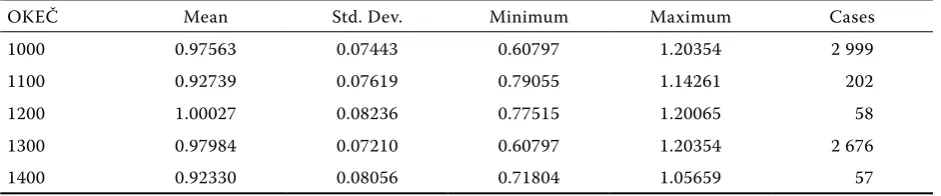
The sum of production elasticities with optimal management is equal to 0.97563, and with the ac-tual management to 1.02604. That is, for an average company in the full sample, there is no indication of the economies of scale for both optimal and actual management, since the sum of the elasticities is about one. however, the situation is different for the indi-vidual branches. Table 3 provides information about the production elasticities in animal production (AnP), plant production (PlP), combined production (coP) and other production (otP). The average company in the plant production has decreasing returns to scale (0.92739), and so does the average company in other production (0.92330). This suggests that the impact of the scale effect on a productivity change could be relatively high when compared to animal and combined production. There is no indication of the economies of scale for the average company in animal and combined production. however, Table 4 shows that the differences among companies are large in all branches.

[image:6.595.72.531.89.203.2]

Finally, if management is considered to be a pro-duction factor, there is a dramatic change in the

Table 3. Production elasticities (with mi) and returns to Scale* (rTS)

  oKEČ

1000 – Agriculture 1100 – PlP 1200 – AnP 1300 – coP 1400 – otP

A 0.22872 0.22154 0.26606 0.22879 0.21558

L 0.05557 0.05636 0.04432 0.05547 0.06566

c 0.05282 0.04500 0.00781 0.05464 0.03762

M 0.63853 0.60450 0.68209 0.64094 0.60444

rTS 0.97563 0.92739 1.00027 0.97984 0.92330

[image:6.595.64.535.652.750.2]

*The calculations are carried out on the sample mean of the given branch, i.e., for the average company in the branch Source: own calculations

Table 4. Descriptive statistics of returns to Scale

oKEČ Mean Std. Dev. Minimum Maximum cases

1000 0.97563 0.07443 0.60797 1.20354 2 999

1100 0.92739 0.07619 0.79055 1.14261 202

1200 1.00027 0.08236 0.77515 1.20065 58

1300 0.97984 0.07210 0.60797 1.20354 2 676

1400 0.92330 0.08056 0.71804 1.05659 57

economies of scale. The direct effect of management is given by:

it xm tm i mm m i

it _m

m

y _{   tβ lnx}



 

 

) ( )

(

ln

(14)

For the average company in the full sample, the direct effect of management is 0.14022 for the op-timal management and 0.16587 for the actual man-agement. This suggests that if management enters the production function as a production factor, the agricultural company has increasing returns to scale. however, the interpretation of marginal values of management is difficult, since management does not have explicitly defined units. on the other hand, the results suggest that management might be consid-ered to be an important determinant of agricultural production.

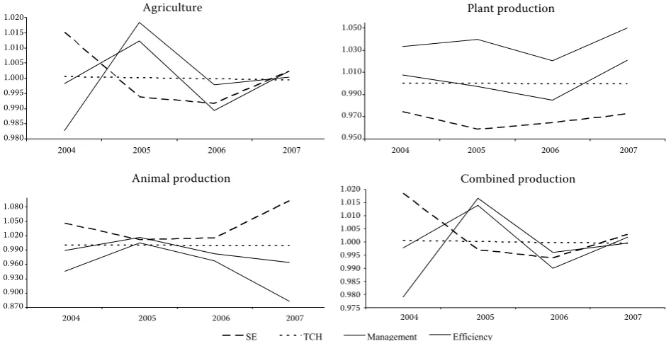
Technical efficiency development

The development of technical efficiency and its components for agriculture and its sectors is shown in Figure 1. We may observe that the development of efficiency in czech agriculture was considerably volatile for the years 2004–2007. Technical efficiency increased in 2005 and decreased in the following year. in 2007, the level of technical efficiency returned to roughly the level it had in 2004. To be precise, technical efficiency experienced only a small increase in the analysed pe-riod, compared to the years 2004 and 2007.

The rather random development in technical ef-ficiency might be a result of adjustment processes connected with the accession to the EU since it can be expected that important changes in the institutional and economic environments demanding adjustments in the organisational structure and structure of inputs of agricultural companies have had a negative impact on technical efficiency. This and the other factors determining the development of technical efficiency are identified based on the breakdown of technical efficiency into its components.

The breakdown shows that the development of technical efficiency and its variability was especially determined by the management and scale effects. Technological change did not contribute signifi-cantly to the efficiency development in the analyzed period. however, its constant trend, together with the symmetry of technical change distribution, suggests that the gap between the best and worst agricultural companies did not change within the analyzed period. The negative impact of manage-ment could be connected with the entrance of the czech republic into the EU in 2004. The positive scale effect might be a result of the positive impact of weather. The yield in almost all branches of plant production was close to record values. The other years were also significantly predetermined by the impact of weather, on the qualitative side of produc-tion as well as the quantitative side. in particular, production in 2006 was negatively influenced by the extreme weather.

Agriculture

0.980 0.985 0.990 0.995 1.000 1.005 1.010 1.015 1.020

2004 2005 2006 2007

SE TCH Management Efficiency 1.020

1.015 1.010 1.005 1.000 0.995 0.990 0.985 0.980

Plant production

0.950 0.970 0.990 1.010 1.030 1.050

2004 2005 2006 2007

SE TCH Management Efficiency

1.050

1.030

1.010

0.990

0.970

0.950

2004 2005 2006 2007

Agriculture Plant production

Animal production

Animal production

0.870 0.900 0.930 0.960 0.990 1.020 1.050 1.080

2004 2005 2006 2007

SE TCH Management Efficiency

1.080 1.050 1.020 0.990 0.960 0.930 0.900 0.870

2004 2005 2006 2007

combined productionCombined production

0.975 0.980 0.985 0.990 0.995 1.000 1.005 1.010 1.015 1.020

2004 2005 2006 2007

SE TCH Management Efficiency

1.020 1.015 1.010 1.005 1.000 0.995 0.990 0.985 0.980 0.975

2004 2005 2006 2007

Agriculture

0.980 0.985 0.990 0.995 1.000 1.005 1.010 1.015 1.020

2004 2005 2006 2007

[image:7.595.62.536.488.729.2]

SE TCH Management Efficiency

Moreover, Figure 1 shows the development of techni-cal efficiency by sectors. Technitechni-cal efficiency in plant production stagnated between 2004 and 2007. The development was given by the management and scale effects. The positive effect of management suggests that the companies specialized in plant production adjusted better to the institutional and economic changes, and hence could be more competitive in the market compared to producers in animal or combined production. Moreover, the impact of weather, espe-cially the negative impact in 2006, was not so strong in this sector compared to combined production. on the other hand, the negative scale effect, which is the result of the estimated decreasing returns to scale, suggests that the companies are producing at a higher than the optimal scale.

Technical efficiency in animal production entered a decreasing trend in 2005. This trend was significantly determined by management. Both the management and scale effects reflect the situation in the mar-ket. The growing imports of meat, which were not compensated by exports, resulted in the increasing competition in the domestic market. This can be observed beginning from the year 2005. however, the surplus of supply over demand was remarkably large in 2007. The decrease in production that re-sulted from a decline in competitiveness of czech agricultural companies and potentially czech food producers brought about a decrease in technical ef-ficiency, since agricultural companies were left with

unused capacities. The decrease in production can be observed from the increase of the scale effect and the decrease of the management effect.

The development of technical efficiency in com-bined production is almost identical to the devel-opment in the agricultural sector as a whole. That is, the same factors which determine the level of technical efficiency could be mentioned (see above). combining the results, we may state that the technical efficiency of companies with combined production is determined by the same factors as in specialized companies. The diversification of production can decrease the negative effects of those factors which determine animal or plant production. on the other hand, the adjustment processes have a negative impact on technical efficiency and may cause its develop-ment to be volatile.

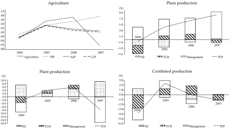
TFP development

Figure 2 shows the development of TFP in agricul-ture and by its sectors. TFP for the total agriculagricul-ture increased between the years 2004 and 2005; however, it entered a decreasing trend in 2005. combined production experienced the same development. TFP in plant production grew during the whole period, as opposed to animal production. The sector of animal production experienced a significant decrease in TFP in the last year of the analyzed period.

–6.00 –5.00 –4.00 –3.00 –2.00 –1.00 0.00 1.00 2.00 3.00

2004

2005

2006 2007

SE TCH Management TFP 3.0

2.0 1.0 0.0 –1.0 –2.0 –3.0 –4.0 –5.0 –6.0

combined production

0.90 0.92 0.94 0.96 0.98 1.00 1.02 1.04 1.06 1.08 1.10

2004 2005 2006 2007

Agriculture PlP AnP CoP 1.10

1.08 1.06 1.04 1.02 1.00 0.98 0.94 0.92 0.90

-5.00% -3.00% -1.00% 1.00% 3.00% 5.00% 7.00% 9.00%

2004

2005 2006 2007

SE TCH Management TFP 9.0

7.0 5.0 3.0 1.0 –1.0 –3.0 –5.0 (%)

-16.00% -14.00% -12.00% -10.00% -8.00% -6.00% -4.00% -2.00% 0.00% 2.00% 4.00% 6.00% 8.00% 10.00%

2004

2005 2006 2007

SE TCH Management TFP 10.0

8.0 6.0 4.0 2.0 0.0 –2.0 –4.0 –6.0 –8.0 –10.0 –12.0 –14.0 –16.0

[image:8.595.66.531.472.738.2]

(%) (%)

Figure 2. TFP development in agriculture and by its sectors Source: own calculations

Agriculture Plant production

The figures for the individual sectors show the break-down of TFP into its individual components. The tech-nical efficiency component is not explicitly shown. Since technical efficiency was analyzed in the previous section, we broke it down, and its components added up to the remaining components of TFP, i.e., the scale effect, technological change and management.

We may observe that all components in plant pro-duction contributed to the increasing trend in the last year, except for technological change. The develop-ment of TFP shows the increasing competitiveness of specialized agricultural companies, which is consistent with the results in the previous section. The nega-tive impact of the scale effect is again a result of the estimated decreasing returns to scale. however, we may observe that agricultural companies are getting closer to the optimal level of scale. in addition, the increase in TFP might be a sign of the positive effects of subsidies in this sector, since subsidies contribute to the competitiveness of producers.

TFP in animal production showed an increasing trend until 2006. This was primarily a result of the positive impact of the technological change and the scale ef-fect. The most important year in the development is the last year. The dramatic drop in the TFP level was a result of all components: technical efficiency, scale effect, technological change and management effect. The drop in production that resulted from decreasing competitiveness in the domestic market was translated into the decline of not only technical efficiency, but also TFP. The calculations show that TFP would decrease even without the technical efficiency component as a result of the reduced production.

The decreasing trend of TFP in combined produc-tion since 2005 is again a result of all components. The reason for the decrease in TFP could by caused by the increasing competition in the sector of animal pro-duction, which resulted from the increasing imports. Since the producers having combined production are, in average, of different technology and technical efficiency, and they are less competitive compared to specialized producers, they might have experienced problems with competitiveness earlier compared to the specialized companies. on the other hand, since these companies can diversify their production, the drop in TFP was not as dramatic as in the case of the specialized producers.

CONCLUSIONS

in this section, we will concentrate on the questions raised in the introduction, namely those regarding the adoption of innovation and the reduced waste

of resources due to the inefficient input use, identi-fication of the key factors which determine the pro-ductivity development in czech agriculture, and the assessment of whether the systemic or idiosyncratic developments in agriculture have occurred.

We estimated that technical change has a positive but declining impact on production. Technical progress was Material using, and Labour, Land and capital sav-ing. Furthermore, technical inefficiency was identified as an important phenomenon in czech agriculture, i.e., the efficiency differences among companies are an important reason for the variations in production; this holds true for both intersectoral and intrasectoral comparisons. Moreover, we identified that manage-ment is an important factor determining production. in particular, it significantly determines the production elasticity of Material, Labour and capital. As far as the economies of scale are concerned, we found that for the average company in the sample, there is no indica-tion of the economies of scale. however, the situaindica-tion is different for the individual branches. Whereas an average company in plant production, as well as other production, has decreasing returns to scale, the sum of production elasticities is about one for the average company in animal and combined production. in ad-dition, the analysis shows that the differences among companies are large in all branches.

The development of technical efficiency is rather random in the total agriculture and combined pro-duction. it stagnated in plant production and experi-enced a decreasing trend in animal production. TFP development for the total agriculture and combined production began to decrease in 2005. Plant pro-duction showed an increasing trend for the whole analyzed period. Animal production experienced a significant drop in TFP in 2007. TFP development was influenced by all components, namely technical efficiency, scale effect, technical change and manage-ment. Their contributions differ intersectorally as well as intrasectorally. The most important factors which determine both technical efficiency and TFP were factors connected with institutional and eco-nomic changes, in particularly a dramatic increase in the imports of meat and increasing subsidies, as well as the impact of weather. Finally, we may conclude that some effects are systemic, i.e., they influence all sectors, but we also identified idiosyncratic factors, especially in animal production.

REFERENCES

inefficiency. Economic Working Papers at centro de Estudios Andaluces E2004/72, centro de Estudios An-daluces.

Álvarez A., Arias c., greene W. (2003): Fixed Management and time invariant technical efficiency in a random coef-ficient model. Working Paper, Department of Economics, Stern School of Business, new York University. caves D.W., christensen L.r., Diewert W.E. (1982):

Mul-tilateral comparisons of output, input and productivity using superlative index numbers. Economic Journal, 92: 73–86.

Čechura L. (2009): zdroje a limity růstu agrárního sek-toru – Analýza efektivnosti a produktivity českého agrárního sektoru: Aplikace SFA (Stochastic Frontier Analysis). (Sources and Limits of growth of Agrarian Sector – Analysis of Efficiency and Productivity of czech Agricultural Sector: Application of SFA –Stochastic Frontier Analysis.) Wolters Kluwer Čr, Praha; iSBn 978-80-7357-493-2.

Čechura L. (2010): Estimation of technical efficiency in czech agriculture with respect to firm heterogeneity. Agricultural Economics – czech, 56: 36–44.

Čechura L., hockmann h. (2010): Sources of Economical growth in czech Food Processing. Prague Economic Papers, (2): 169–182.

curtiss J. (2002): Efficiency and Structural changes in Transition: A Stochastic Frontier Analysis of czech crop Production. [Dissertation.] institutional change in Agriculture & natural resources. Shaker Verlag gmbh, germany; iSBn 3832203656.

Diewert W.E. (1976): Exact and superlative index numbers. Journal of Econometrics, 4: 115–145.

green W. (2007): LiMDEP version 9.0 User’s Manual. Econometric Software, inc.

hockmann h., Pieniadz A. (2008): Farm heterogeneity and Efficiency in Polish Agriculture: A Stochastic Frontier Analysis. in: 12th _{congress of the European} Associa-tion of Agricultural Economists – EAAE 2008, ghent, Belgium.

hughes g. (1999): Total factor productivity of farms struc-tures in central and Eastern Europe. Bulgarian Journal of Agricultural Science, 5: 298–311.

Jelínek L. (2006): Vztah technické efektivnosti a technolo-gické změny v sektoru výroby mléka. (relation between technical efficiency and technological change in milk production.) [Dissertation.] PEF ČzU. Prague.

Jondrow J. et al. (1982): on the estimation of technical inef-ficiency in the stochastic frontier production function model. Journal of Econometrics, 19: 233–238.

Juřica A., Medonos T., Jelínek L. (2004): Structural chang-es and efficiency in czech agriculture in the pre-ac-cession period. Agricultural Economics – czech, 50: 130–138.

Kumbhakar S.c., Lovell c.A.K. (2000): Stochastic Fron-tier Analysis. University Press, cambridge; iSBn 0521666635.

Mathijs E., Blaas g., Doucha T. (1999a): organisational form and technical efficiency of czech and Slovak Farms. MocT-MoST, 9: 331–344.

Mathijs E., Dries L, Doucha T., Swinnen J.F.M. (1999b): Production efficiency and organization of czech Ag-riculture. Bulgarian Journal of Agricultural Science, 5: 312–324.

Mathijs E., Tollens E., Vranken L. (2001): contracting and Production Efficiency in czech Agriculture. Working Paper, catholic University of Leuven.

Medonos T. (2006): investiční aktivita a finanční omezení českých zemědělských podniků právnických osob. (in-vestment activity and financial constraints of czech ag-ricultural companies.) [Dissertation.] PEF ČzU. Prague. němec J., Štolbová M., Vrbová E. (2006): cena zemědělské

půdy v České republice v letech 1993–2004. (Price of Agricultural Land in the czech republic in year 1993– 2004.) VÚzE, Prague; iSBn 80-86671-25-9.

Arrived on 25th _{March 2011}

Contact address: