Processing of conventional soil survey data using geostatistical methods

A large set of data from the conventional soil survey carried out in the past on one hand, and existence of modern technologies for data process-ing on the other hand, require findprocess-ing ways of ex-ploitation of these relatively easily available data. Different aims and methods of conventional soil survey and geostatistics can cause problems for the exploitation of these data. This paper is focused on outlining the major problems that arise, and finding an appropriate solution to overcome the gaps.

Conventional soil survey

A conventional soil survey was carried out in the former Czechoslovakia in the 1960’s. This soil survey covered all agricultural land. The urban and forest land was excluded. A sampling scheme of soil pits was generated to describe all soil clas-sification units. The landscape was divided into three categories according to geomorphology and lithology (Němeček et al. 1967). These three cat-egories differ in the density of soil pits. The first category represents the most homogenous land-scape – flat or slightly hilly areas with relatively homogenous soil-lithogenic properties. The second category represents moderately hilly landscape, areas influenced by water erosion, areas with heterogeneous lithography and mountains. The

third category includes river alluvia, areas with extremely heterogeneous soil-lithogenic conditions and soils affected by salinity. The density of soil pits in given categories is in Table 1.

There were three types of profile pits according to the set of determined characteristics (Němeček et al. 1967). The base profile pits characterize lower map units. Samples were taken only from topsoil and subsurface layer. Clay content and pH were determined. The selective profile pits describe soil-mapping units given by genetic and expressive lithogenic features. The samples were collected from all horizons in the profile. Clay content, pH, CEC, base saturation, organic carbon content and some other properties were measured. The special profile pits provide a wide number of chemical and physical soil properties (e.g. mineralogy).

The locations of the base profiles were determined so that they described typical parts of relief and all typical soil taxonomy units. The location of selec-tive profiles was chosen so that they represented typical classification units and their lithogenic variants. In both cases, if the limit of the soil pits (according to Table 1) was not reached, the rest of soil pits was distributed to cover the area as homogenously as possible.

This sampling design represents a typical con-ventional soil survey, where the soil pits are not randomly distributed over the area. Surveyors select

Processing of conventional soil survey data

using geostatistical methods

V. Penížek, L. Borůvka

Czech University of Agriculture in Prague, Czech Republic

ABSTRACT

The aim of this study is to find a suitable treatment of conventional soil survey data for geostatistical exploitation. Different aims and methods of a conventional soil survey and the geostatistics can cause some problems. The spatial variability of clay content and pH for an area of 543 km2 _{was described by variograms. First the original untreated} data were used. Then the original data were treated to overcome the problems that arise from different aims of conventional soil survey and geostatistical approaches. Variograms calculated from the original data, both for clay content and pH, showed a big portion of nugget variability caused by a few extreme values. Simple exclusion of data representing some specific soil units (local extremes, non-zonal soils) did not bring almost any improvement. Exclu-sion of outlying values from the first three lag classes that were the most influenced due to a relatively big portion of these extreme values provided much be�er results. The nugget decreased from pure nugget to 50% of the sill variabi-lity for clay content and from 81 to 23% for pH.

Keywords: conventional soil survey; geostatistics; data processing; spatial variability

the distribution of sampling sites subjectively. Such designs are purposive and non-random, and do not provide statistical estimates (Hengl 2003). The problems arising from it are discussed later.

Geostatistics

Geostatistics is a technology for estimating the local values of properties that vary in space (Oliver and Webster 1991). The theory is based upon the concept of a random variable, which expresses a continuous variable depending on a location (Stein et al. 1998). It is expected that observations close together in space will be more alike than those further apart (Lloyd and Atkinson 1998).

Variogram (also known as semivariogram) is the most commonly used measure of spatial variation in geostatistics. The semivariance, denoted by γ, at a given separation is half the expected square difference between values at that separation:

γ(h) = 0.5E [{Z(x) – Z(x + h)}2_]

where: Z(x) and Z(x + h) are the values of Z at any two places, x and x + h, separated by h, a vector having both distance and direction (lag) (Oliver and Webster 1991).

The shape of a variogram is characterized by three parameters – nugget, range, and sill. Nugget represents the part of the variability that is not spatially dependent. The maximum semivariance value, where the semivariance does not increase any further, is called the sill. The distance where the sill is reached is the range. The variogram is used for interpolation (most widely used is ordi-nary kriging) and for measuring the confidence of the estimates (van Groenigen 2000).

There are several sampling strategies that are used in geostatistics. Regular grids, both triangular and rectangular, are presented by many authors (van Groenigen et al. 2000, Webster and Oliver 2000, Frogbrook et al. 2002) as one of the possi-bilities. A nested or random sampling scheme is another way of obtaining data for geostatistical Table 1. Density of soil profile pits for different

geomorpho-logic-lithographic categories

Landscape category

Number of hectares per one base

profile pit

Number of hectares per one selective

profile pit

I. 18 180

II. 12 120

III. 7 70

methods (Webster 1977, Oliver and Webster 1991, Wollenhaupt et al. 1997); van Groenigen (2000) presents methods that are used for optimization of sampling grids. Different criteria for optimization of sampling scheme are chosen for decreasing the uncertainty of the prediction of spatial dependence values.

MATERIAL AND METHODS

Data and the study site

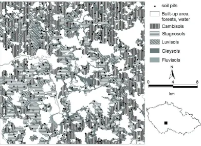
The study area is located in the district of Tábor in Southern Bohemia (Figure 1). The area of interest is represented by a rectangle section of 543 square kilometers. Cambisols are the prevailing soil clas-sification unit (45.1%). Stagnosols cover 26.2%, Luvisols 15.0%, Gleysols 7.5%, and Fluvisols 3.2%. Geology of the area is formed mainly by granites, gneisses, loesses and alluvial sediments. The elevation of the area ranges from 410 to 670 m above sea level.

In this section, 257 selected profiles were located and were used for this project. Clay content and pH in subsurface horizon were used as representative spatial variables.

Methods

The variability of clay content and soil pH was described by experimental variograms. The lag

classes were set up to obtain in each lag class a sufficient amount of pairs of the values to de-scribe the variability. The variograms were mod-eled by weighted least squares approximation. Geostatistical analysis of source data was done using GS+ _{software (Robertson 2000).}

First the original untreated data were used. Then the original data were treated to overcome the prob-lems that arise from different aims of conventional soil survey and geostatistical approaches. The ex-treme values of semivariability were examined and processed. This examination was focused on pits from places with extreme lithogenic conditions and non-zonal soils. Processing of the data was based on different ways of excluding extreme data.

RESULTS AND DISCUSSION

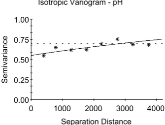
Variograms based on the original data, both for clay content and pH, showed a big portion of nugget variability (Figure 2). The high nugget variability would indicate that there is no spatial dependence of the soil properties or the spatial dependence is very low. Detailed examination of the variogram show that the high nugget vari-ability in the lag classes representing the shortest distances is caused by a few extremes. These few outlying values radically influence the shape of the variogram. Figure 3 presents the variance cloud for the first three lag classes of clay content. Extreme values (outliers) are present in lag classes for bigger distances as well (Table 2). However, the proportion

0 35 70 105 140

0 1000 2000 3000 4000

Semivariance

Separation Distance Isotropic Variogram - clay content

0.00 0.25 0.50 0.75 1.00

0 1000 2000 3000 4000

Semivariance

Separation Distance Isotropic Variogram - pH

Figure 2. Variogram from original untreated data for clay content and pH

Table 2. Occurrence of outlying values of variability within the lag classes (clay content)

Separation distance (m) 500 1000 1500 2000 2500 3000 3500 4000

Number of outlying values 4 5 5 6 8 7 9 8

0 569 1138 1706 2275

0 125 250 375 500

Va

ria

nc

e

Separation Distance Variance Cloud (Isotropic Lag Class 1)

0 990 1980 2970

500 625 750 875 1000

Va

ria

nc

e

Separation Distance

Variance Cloud (Isotropic Lag Class 2)

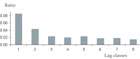
of these extreme values to other values belonging to given class is much lower. The ratio between outlying and normal values within lag classes is presented in Figure 4. It is obvious that the first two lag classes in variogram for clay content are the most affected. The expectation based on the spatial random variable theory would be that the variability in the first two lag classes would be the lowest. In fact the opposite is true.

The relatively high proportion of extreme val-ues in the first three lag classes is caused by two factors: 1) the amount of pairs, which represent the variability, is relatively low. The average variability within the lag class can be therefore easily influenced by a few extremes. 2) The con-figuration of sampling scheme of the data is not

random. The original sampling scheme described above provides closely located extreme values. In homogenous areas, the sampling scheme is sparse and no closely located values that would show low variability are available. On the other hand, in the areas with high heterogeneity, points lie closer to each other. The reason for this is that they describe areas that strongly differ. One of the values of such closely lying pairs of values represents local lithogenic or landform extremes on relatively small areas. The second example of these extremes is non-zonal soils like Fluvisols and Gleysols. These soils represent narrow strips around small streams. This influence of extremes is more important at shorter distances.

When the medium to small-scale variability of the soil properties is to be described, it is reasonable to exclude values that represent these small areas with lithogenic or landform extremes. Describing the properties of non-zonal soils by geostatistics is also very problematic. With the data available for this study, it is not possible. Because of the shape and extent of these soils, the data representing them can be excluded as well.

Two approaches of excluding the extremes can be applied. The first approach is to exclude all data representing soil units that are a source of extreme variability. This can be done when these soil units represent only areas with small extent, which would be not mapped anyway. The decision of what soil units can be excluded or not is based on individual decision. This decision must take into consideration the aim of the project, the scale of the resulting materials and so on. The second approach is to find the outlying values using the variance clouds for the individual lag classes of the variogram and exclude these extreme values. Which of the values from the pair representing the variability would be excluded should be done ac-cording to what soil units or subunits it belongs to. Both these approaches were tested. Simple exclu-sion of data representing soil units with extreme features (46 pits – 9 Fluvisols and 37 Gleysols) did not bring almost any improvement (Figure 5). The total variability decreased. The shape of the

vario-Figure 4. Ratio between outlying values and other values within the lag classes – clay content

0 1019 2039 3058

1000 1167 1333 1500

Va

ria

nc

e

Separation Distance Variance Cloud (Isotropic Lag Class 3)

Figure 3. Variance cloud for the first three lag classes for clay content; the dashed line separates the extreme variance values

Ratio

gram was the same even if there was a decrease of semivariability in the first two lag classes.

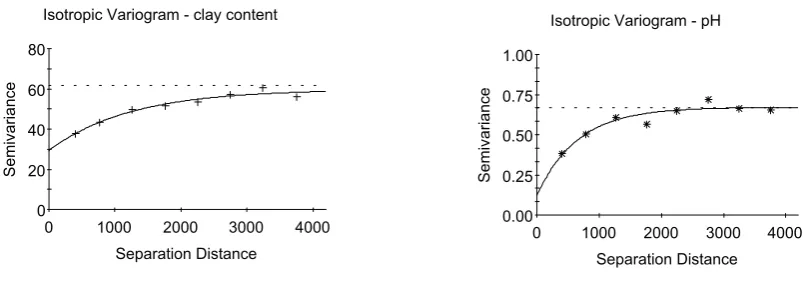
Exclusion of outlying values provided much better results. For this purpose, the variance cor-responding to one half of the maximum difference between a pair of values in the dataset was used as a limit for outlier distinguishing. In the case of clay content, maximum value was 56%; minimum value was 0%. One half of the difference was 28 and the limit variance calculated as the square of the difference (Robertson 2000) was thus 784. All variances exceeding this value in each class were considered as outliers (Figure 3). The outlying val-ues from the first three lag classes were excluded (4 from first class and 5 from second and third class), since the influence in these classes is the most significant due to a small number of values in these classes. For the second class, 5 removed outlying values in the original dataset appeared as 6 outliers in the variance cloud, because one of the values provided high variances with two other values in this lag class. Even when only a small number of data was excluded (Table 2),

the shape of variogram changed apparently. The nugget decreased from pure nugget to a 50% of the total variability for clay content and from 81 to 23% for pH (Figure 6).

The results showed how easily the semivariance could be influenced, when lag classes contain rela-tively small number of data. The exploitation of the base profile data could be a possible way how to avoid these problems. Base profiles can provide a large set of data that are closely located to each other and that suitably describe the semivariance.

This study presents that the exploitation of data originating from conventional soil survey is possible but the initial processing of the data is a necessary step for further exploitation of these data.

REFERENCES

Frogbrook Z.L., Oliver M.A., Salahi M., Ellis R.H. (2002): Exploring the spatial relations between cereal yield and soil chemical properties and the implications for sampling. Soil Use Manage., 18: 1–9.

Figure 6. Variogram from data for clay content and pH treated by excluding concrete outliers

0 18 35 53 70

0 1000 2000 3000 4000

Se

m

iv

ar

ia

nc

e

Separation Distance Isotropic Variogram - clay content

Figure 5. Variogram from data for clay content and pH treated by excluding minor soil units and subunits

0.00 0.18 0.35 0.53 0.70

0 1000 2000 3000 4000

Semivariance

Separation Distance Isotropic Variogram - pH

0 20 40 60 80

0 1000 2000 3000 4000

Se

m

iv

ar

ia

nc

e

Separation Distance Isotropic Variogram - clay content

0.00 0.25 0.50 0.75 1.00

0 1000 2000 3000 4000

Se

m

iv

ar

ia

nc

e

Groenigen J.W. van (2000): Constrained optimalisation of spatial sampling: a geostatistical approach. ITC Publ. Ser., Wageningen.

Groenigen J.W. van, Gandah M., Bouma J. (2000): Soil sampling strategies for precision agriculture research under sahelian conditions. Soil Sci. Soc. Am. J., 64: 1674–1680.

Hengl T. (2003): Pedometric mapping: bridging the gaps between conventional and pedometrical approaches. [Ph.D. Thesis.] The Wageningen Univ.

Lloyd Ch.D., Atkinson P.M. (1998): Scale and the spatial structure of landform: optimizing sampling strategies with geostatistics. http://www.ai-geostats.org/papers [cit. 2004-01-15].

Němeček J., Damaška J., Hraško J., Bedrna Z., Zuska V., Tomášek M., Kalenda M. (1967): Soil survey of ag-ricultural lands of Czechoslovakia. 1st _{Part. MZVZ,} Praha. (In Czech)

Oliver M.A., Webster R. (1991): How geostatistics can help you. Soil Use Manage., 7: 206–217.

Robertson G.P. (2000): GS+: Geostatistics for the environ-mental sciences. Gamma Design Software, Plainwell, Michigan, USA.

Stein A., Bastiaanssen W.G.M., Bruin S. de, Cracknell A.P., Curran P.J., Fabbri A.G., Gorte B.G.H., Groeni-gen J.W. van, Meer F.D. van der, Saldana A. (1998): Integrating spatial statistics and remote sensing. Int. J. Remote Sens., 19: 1793–1814.

Webster R. (1977): Quantitative and numerical meth-ods in soil classification and survey. Clarendon Press, Oxford.

Webster R., Oliver M.A. (2000): Geostatistics for envi-ronmental scientists. John Wiley & Sons, Chichester. Wollenhaupt N.C., Mulla D.J., Gotway-Crawford C.A.

(1997): Soil sampling and interpolation techniques for mapping spatial variability of soil properties. In: Pierce F.J., Sadler E.J. (eds.) (1995): Symp. The state of site specific management for agriculture, St. Louis, Missouri: 19–53.

Received on February 3, 2004

ABSTRAKT

Zpracování dat tradičního půdního průzkumu geostatistickými metodami

Odlišné cíle a postupy tradičního půdního průzkumu a geostatistických metod způsobují problémy s využitím těchto dat. Tento příspěvek je zaměřen na možnosti odstranění problémů spojených s odlišným přístupem tradičního půd-ního průzkumu a geostatistických metod k odběru vzorků. Byla popsána prostorová variabilita obsahu jílu a pH jak pro původní neupravená data Komplexního průzkumu zemědělských půd, tak i pro data upravená. Původní data vykázala vysokou variabilitu obou zkoumaných vlastností i na malé vzdálenosti. Tato variabilita byla způsobena výskytem extrémních hodnot (i když malého množství). Odstranění dat reprezentujících půdní jednotky, způsobující tuto velkou variabilitu (azonální půdy niv a lokální extrémy dané morfologií terénu a složením substrátu), nevedlo k výraznému zlepšení. Odstranění extrémních hodnot semivariance na základě podrobné analýzy dat přispělo k pod-statně lepším výsledkům. Podíl semivariance, která zdánlivě není prostorově závislá, klesl u obsahu jílu ze 100 % na polovinu a u pH z 81 na 23 %. Výsledky ukazují, že využití dat tradičního půdního průzkumu geostatistickými metodami je možné, ale předběžné zpracování těchto dat je nezbytným krokem pro jejich správné použití.

Klíčová slova: půdní průzkum; geostatistika; zpracování dat; prostorová variabilita

Corresponding author: