http://wrap.warwick.ac.uk/
Original citation:
Bruen, Thomas and Marco, James. (2016) Modelling and experimental evaluation of
parallel connected lithium ion cells for an electric vehicle battery system. Journal of
Power Sources, 310. pp. 91-101. ISSN 0378-7753
Permanent WRAP url:
http://wrap.warwick.ac.uk/76878
Copyright and reuse:
The Warwick Research Archive Portal (WRAP) makes this work by researchers of the
University of Warwick available open access under the following conditions.
This article is distributed under the terms of the Creative Commons Attribution 4.0
License (
http://creativecommons.org/licenses/by/4.0/
) which permits any use,
reproduction and distribution of the work without further permission provided the original
work is attributed.
A note on versions:
The version presented in WRAP is the published version, or, version of record, and may
be cited as it appears here.
Modelling and experimental evaluation of parallel connected lithium
ion cells for an electric vehicle battery system
Thomas Bruen
*, James Marco
WMG, University of Warwick, Coventry, CV4 7AL, UK
h i g h l i g h t s
Experimental evaluation of energy imbalance within parallel connected cells. A validated new method of combining equivalent circuit models in parallel. Interdependence of capacity, voltage and impedance for calculating cell currents. A 30% difference in impedance can result in a 60% difference in peak cell current. A difference of over 6% in charge throughput was observed during cycling.
a r t i c l e i n f o
Article history:
Received 24 July 2015 Received in revised form 17 November 2015 Accepted 1 January 2016 Available online xxx
Keywords:
Electric vehicle Lithium ion Battery pack
Battery management system Equivalent circuit model
a b s t r a c t
Variations in cell properties are unavoidable and can be caused by manufacturing tolerances and usage conditions. As a result of this, cells connected in series may have different voltages and states of charge that limit the energy and power capability of the complete battery pack. Methods of removing this energy imbalance have been extensively reported within literature. However, there has been little dis-cussion around the effect that such variation has when cells are connected electrically in parallel. This work aims to explore the impact of connecting cells, with varied properties, in parallel and the issues regarding energy imbalance and battery management that may arise. This has been achieved through analysing experimental data and a validated model. The main results from this study highlight that significant differences in currentflow can occur between cells within a parallel stack that will affect how the cells age and the temperature distribution within the battery assembly.
©2016 The Authors. Published by Elsevier B.V. This is an open access article under the CC BY license (http://creativecommons.org/licenses/by/4.0/).
1. Introduction
Cells in a battery pack may be electrically connected in parallel in order to increase the pack capacity and meet requirements for power and energy[1,2]. For example, the Tesla Model S 85 kWh battery pack uses 74 3.1 Ah cylindrical cells to create a parallel unit, and 96 of these units in series. Conversely, the Nissan Leaf 24 kWh battery pack consists of 33 Ah cells, with 2 in parallel and 96 in series [3]. The nature of a parallel connection means that the voltage over each cell is the same and the applied current is equal to the sum of the individual cell currents. It is commonly assumed that energy balancing is only required for cells in series[4,5]since the cells in a parallel unit are inherently balanced due to the common
voltage[6,7]. However, there has been little experimental data to explore this further. Variations in internal resistance mean that the cells within a parallel unit will undergo different currents. How-ever, individual cell currents are typically not measured, and so any variation in current is not detected by the battery management system (BMS). Differences in current can change the state of charge (SOC), temperature and degradation rate of each cell[8,9], meaning cells in parallel may not be at the same SOC despite being at the same terminal voltage[10], and could degrade at different rates. State of health (SOH) is often used to quantify cell degradation, with common definitions using the increase in resistance or decrease in capacity relative to when the cell is new[11]. Accurate SOH esti-mation is a key challenge for battery management systems (BMSs)
[12].
The objective of this paper is to introduce a model that allows for thorough analysis of parallel-connected cells in a battery pack, while integrating with existing frameworks. This can be used to aid
*Corresponding author.
E-mail addresses: [email protected] (T. Bruen), james.marco@ warwick.ac.uk(J. Marco).
Contents lists available atScienceDirect
Journal of Power Sources
j o u r n a l h o m e p a g e : w w w . e l s e v i e r . c o m/ l o ca t e / j p o w s o u r
http://dx.doi.org/10.1016/j.jpowsour.2016.01.001
battery pack design, for example evaluating different series-parallel configurations of cells, and analysis of the temperature distribution within the battery pack. The robustness of BMS functions such as SOC estimation and fault detection can also be tested.
Gogoana et al. [13] cycle-aged two cylindrical lithium iron phosphate (LFP) cells connected in parallel. They found that a 20% difference in internal resistance resulted in a 40% reduction in the useful life of the pair of cells compared to if the cells had approximately equal internal resistances. The authors attribute this to the uneven current distribution between the cells. Their results highlight that each cell will go through periods where it experiences high currents that will in turn age the cells more quickly. Gong et al. [1] drew similar conclusions from their experimental work with 32 Ah cells. When two cells with a 20% impedance difference were connected in parallel, the peak current experienced was 40% higher than if the cells were identical. The authors also performed simulation studies, using the Mathwork's Simscape extension to Simulink to connect two equivalent circuit models (ECMs) in parallel. This is one of the few examples of parallel cell modelling within the literature. Wang et al. also used Simscape for modelling cells in parallel[14], although the current distribution was not analysed in detail. Offer at al. used a simple cell model in Simscape for analysing the effect of poor connection resistance between parallel cells [15]. This effect was explored further in Ref.[10], where an electrochemical model was used to simulate the impact interconnection resistance between cells in parallel has on battery system performance. Often, a parallel unit
‘lumped’model is created, where the parameters of a single cell model are scaled to create an effective parallel unit, such as in Ref. [16], in which the authors screen a large batch of cells to ensure that only similar cells are connected in parallel. While this may be valid for new cells, there is no guarantee that the cells will degrade in the same way, as demonstrated in Ref. [17]. Similar assumptions are made in Ref. [6], where the SOC of cells in a parallel is assumed to always be equal. While assumptions such as these allow for the high-level simulation of a battery pack, it as-sumes the cells within a parallel unit are identical and as such all experience the same electrical and thermal loading. This limits the accuracy of the model and means that some potential physical phenomena, such as temperature gradients and current variations, are not analysed and accounted for as part of a model-based design process. While an acausal approach such as Simscape can account for variations in parameters, it is less well suited to analysis and manipulation than solving a system of ordinary dif-ferential equations (ODEs), as is the case for a single cell model.
The contribution of this paper is to extend the existing literature in terms of both simulation method and experimental data. In Section2a generic parallel cell model is derived, which allows for the calculation of cell currents and states within a parallel stack while maintaining the same model structure as a single cell model. This means that cells in parallel can be modelled and evaluated within conventional frameworks without having to make as-sumptions about cell uniformity. The experimental work is intro-duced in Section 3, in which four commercially available 3 Ah 18650 cells are aged by different amounts to create differences in their respective capacity and impedance. The cells are then con-nected in parallel and cycle-tested to analyse and quantify the variations in performance, such as current and temperature, which arise from these differences. The model is validated against experimental data in Section4. Results from the experimental and simulation studies are analysed in Section 5, in which various vehicle usage cases are considered and the impact of using cells in parallel for these applications is evaluated. Conclusions and further work are presented in Section6.
2. Model development
The ECM is commonly used to simulate the voltage response of individual cells, due to its relative simplicity, ease of parameter-isation and real-time feasibility[18,19]. The primary aim of the ECM is to match the voltage response of a physical cell based on a current input, rather than to model the cell using fundamental electrochemical theory. Despite the lack of a physical basis to the model, elements of the circuit can be related to aspects of the cell's physical response, such as charge transfer and diffusion
[20].
2.1. Equivalent circuit model
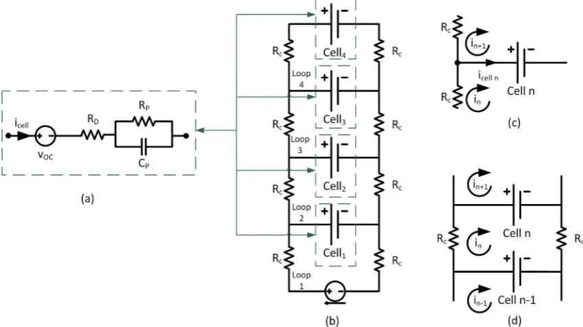
The single cell ECM consists of several elements, as shown in
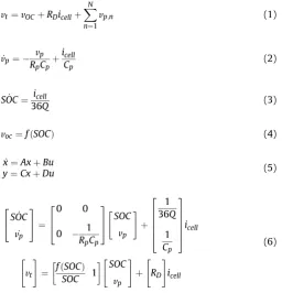
Fig. 1a: the open circuit voltagevOC, internal resistanceRDand a resistor-capacitor (RC) pair, which is a resistorRpand capacitorCpin parallel. Multiple RC pairs in series can be used depending on the bandwidth andfidelity of the response required. Eq.(1)shows that for a given currenticell, the terminal voltagevtis comprised of the
vOC, the voltage over the internal resistance and the sum of the RC pair voltagesvp.vpandSOCare governed by ODEs, given by(2)and (3)respectively. Typically,vOCis not calculated directly; insteadSOC is calculated using(3), whereQis the cell capacity in Ah, andvOC found from(4). Unlike(3), thevOC-SOCfunction in (4) is typically nonlinear. By treatingSOC, notvOC, as a model state variable, the state equations are kept linear. Commonly, systems such as this are written in state-space form as in(5). The system for one RC pair is shown in linear state-space form in(6). Throughout this paper, a one-to-one relationship between SOC and vOChas been assumed, which can often be considered sufficiently accurate[21]. In reality the cell response may exhibit hysteresis, in which thevOCat a given SOC may be different depending on whether the cell is being charged or discharged. As discussed in Ref. [22], this can be accounted for by adding additional states (ODEs) to the model.
vt ¼vOCþRDicellþ XN
n¼1
vp;n (1)
_
vp¼ vp
RpCpþ icell
Cp (2)
_ SOC¼ icell
36Q (3)
voc¼fðSOCÞ (4)
_
x¼AxþBu
y¼CxþDu (5)
2 4SOC_
_ vp 3 5¼ 2 6 4 0 0
0 1
RpCp 3 7 5 " SOC vp # þ 2 6 6 6 6 4 1 36Q 1 Cp 3 7 7 7 7 5icell
" vt
# ¼
fðSOCÞ
[image:3.595.301.558.466.733.2]2.2. Parallel equivalent circuit model
The ECM in Section 2.1 can be expanded to incorporate any number of cells in parallel. For this derivation, four cells with one RC pair each is used, but the methodology is generic and can be extended to any number of cells or RC pairs.Fig. 1b presents a schematic of four cells in parallel with an interconnection resis-tance (Rc) between each terminal. Each cell is represented by its own ECM as inFig. 1a.
In addition to the state equations for the single cell, there are also algebraic constraints on the parallel cell system. These are based on Kirchoff's laws for current and voltage. The currents at a junction must sum to zero, which for the parallel cell system occurs at the cell connections, as shownFig. 1c. ForNcells, Eq.(7) de-scribes the relationship between loop currents i1 to iN and cell currentsicell 1toicell N. The two cases arise due to there being noinþ1 for thefinal cell.
icell n¼
ininþ1;n<N
in;n≡N (7)
Similarly, the voltages around a loop must sum to zero. A typical loop for cellnis shown inFig. 1d. There areN-1loops to solve, as the
first loop current is the current source and is therefore trivial. The voltage loop equation is given by(8), and can be expanded to(9)by defining the cell voltage through its constituent components ac-cording to(1).
vt nvt n1þ2Rcin¼0 (8)
In order to work with the algebraic equations in (9) it is convenient to usevOCas a state rather thanSOC. This moves the nonlinear function from the output matrixCto the input matrixB, but does not affect the state matrix Aand so the system poles remain unchanged. To achieve this, an effective capacitance,C0is defined, which determines how much charge is required to cause a given change in vOC. As it can be seen in (10), C0 is found by calculating the gradient of thevOC-SOCcurve and factoring in cell capacityQin Ah. The resulting state equation is given by(11). This equation is still an integrator like Eq.(3), and there is no change in the overall transfer function of the system. The cell equations now take the form of(12).
C0ðvOCÞ ¼36QdSOCdvOCðvOCÞ (10)
_ vOC¼icell
C0
(11)
2 6 4vOC_
_ vp
3 7
5¼
2 6 4
0 0
0 1
RpCp 3 7 5 "
vOC vp
# þ
2 6 6 6 6 4
1
C0
1
Cp 3 7 7 7 7 5icell
" vt
#
¼ ½1 1 "
vOC vp
# þ
" RD
# icell
(12)
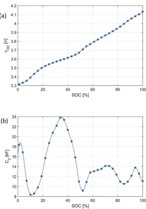
[image:4.595.89.514.70.308.2]Fig. 2a showsvOCas a function ofSOCfor the cell type employed for this research.Fig. 2b then shows how this is translated into a Fig. 1.(a) Equivalent Circuit Model; (b) Schematic of four cells connected in parallel; (c) Mesh junction for celln; (d) Mesh Loop for celln.
0¼
vOC nvOC n1þvp nvp n1þRD nðininþ1Þ RD n1ðin1inÞ þ2Rcin;n<N
[image:4.595.308.499.492.652.2]C0eSOCcurve through applying(10). It can be seen that a largerC0 value corresponds to aflatter gradient at that point of thevOC-SOC curve, since in this region more charge is required to create a given change invOC. TheC0curve is less smooth than thevOCcurve and care must be taken in terms of data acquisition and interpolation method to ensure the gradient remains accurate. This is particularly the case for LFP cells, wherevOC-SOCcurve is known to have aflat region, which will result in a large value ofC0[23].
The individual cell state equations in(12)can be merged to form one larger solution as in(13)by creating block diagonals of each matrix and concatenating the state and input vectors. Despite there now beingNcells andNinputs, the output (vt) is the same for all cells and so the output equation for any single cell can be applied rather than calculating all of them. In this case the output equation for thefirst cell has been applied.
2 6 6 6 6 4 _ x1 _ x2 « _ xN 3 7 7 7 7 5¼ 2 6 6 4 A1 A2 1 AN 3 7 7 5 2 6 6 4 x1 x2 « xN 3 7 7 5þ 2 6 6 4 B1 B2 1 BN 3 7 7 5 2 6 6 4
icell;1
icell;2
«
icell;N 3 7 7 5
vt¼ ½C1 0 0 … 0
2 6 6 4 x1 x2 « xN 3 7 7
5þ ½D1 0 0 … 0
2 6 6 4
icell;1
icell;2
«
icell;N 3 7 7 5
(13)
By analysing the structure and resulting Eigenvalues of the
system state matrix of(13)it can be seen that the dynamics of each cell remain independent, and an input vector of cell currents is required. However, cell currents are typically not measured and so instead the system input needs to be the scalar measured currenti1. This is achieved by writing the voltage loop algebraic Eq.(9)in matrix form as in(14). This introduces three matrices: the resis-tance matrixR, which is a tridiagonal square matrix of cell and interconnection resistances, the state dependency matrixE, which uses the state vector to create the voltage differences and the input dependency vectorFto account fori1.
R 2 6 6 4 i1 i2 « iN 3 7 7
5¼ExþFi1
R¼ 2 6 6 4
1 0 0 0
0 RD;1þRD;2þ2Rc
RD;2 0
0 RD;2 1 RD;N1
0 0 RD;N1
RD;N1þRD;Nþ2Rc 3 7 7 5 E 2 6 6 4
0 0 … … 0
1 1 1 1 0 … 0
0 … 1 1 1 1 0 0
0 … 0 1 1 1 1
3 7 7 5 F¼ 2 6 6 6 6 4 1 RD;1þ2Rc
0 « 0 3 7 7 7 7 5 (14)
By invertingR, a vector of loop currents can be solved for. Eq.
(15)introduces the current translation matrixG, to calculate the individual cell currents from the loop currents in(14), i.e. applying
(7)in matrix form. This shows that the cell currents can be written as a function of the cells' states and the input current.
2 6 6 4
icell1 icell2
«
icell N 3 7 7
5¼GR1ðExþFi1Þ
G¼ 2 6 6 4
1 1 0 0
0 1 1 0
0 1 1 1
0 … 0 1
3 7 7 5
(15)
The cell current vector in(15)is also the input vector for(13)and so can be substituted to create(16). For convenience, the solution can be grouped into state and input components to give the augmented state-space solution in(17). These equations demon-strate that the states of all cells in parallel can be written using the same inputs and outputs as for a single cell. This facilitates the use of established control theory methods and also enables a more thorough analysis of the individual and collective response of cells when connected in parallel.
_
x¼AxþBGR1ðExþFi1Þ
i
y¼CxþDGR1ðExþFi1Þ
i (16)
_
x¼A0xþB0i1
y¼C0xþD0i1
A0¼AþBGR1E B0¼BGR1F
C0¼CþDGR1E
D0¼DGR1F
(17)
[image:5.595.36.282.60.411.2]Established control theory states that the system poles for a Fig. 2.(a): vOCas a function of SOC for the cell under test; (b) Effective capacitance (C0)
state-space model can be found using(18). For individual cells, an analytical solution to the eigenvalues is straightforward as theA
matrix is a leading diagonal matrix; the solution is given in(19). However, for the parallel system theA0matrix is full andfinding the eigenvalues analytically is complicated even for a simple case.
p¼eig A0 (18)
p¼
0; 1 RpCp
(19)
Whereas for a single cell model the system pole forVOC(orSOC) is zero, this is no longer the case for the cells in parallel. The self-balancing interactions imply a slow, stable convergence and as such the system contains negative poles to account for this. The self-balancing poles for the parallel system can be approximated by
(20). For the cells used for this work, the time constant for the self-balancing dynamics was in the region of 500e600 s, depending on factors such as impedance and SOC.
pz 1 C0 RDþPnRCn¼1Rp;n
(20)
3. Experimental procedure
The new modelling framework derived in Section2.2requires parameterisation and validation against experimental data to fully explore its accuracy and robustness. Additionally, data from phys-ical cell testing will also help to determine the appropriate band-width of the model, to ensure that the cells' responses, and any interactions, are reliably captured. For the following experimental work, four 3Ah 18650 lithium ion cells were used. The specifics of the data acquisition required for parallel cell measurement is detailed in Section3.1.
3.1. Cell current measurement
A Bitrode MCV16-100-5 was used to control the applied current. However, this equipment cannot measure current through cells in parallel as only the total circuit current applied to the parallel unit is measured. A measure of the unique cell currents is required for analysis purposes as well as to validate the model. To measure the current through each cell, a 10 m
U
shunt resistor with less than 500 ppm K1thermal sensitivity was connected in series with each cell. This has the disadvantage of changing the resistance of each string, meaning the absolute value of current through each cell is different than if the shunt resistors were not in the circuit. Hall-effect sensors can be used to sense current without being a part of the circuit and so do not impact the result. However, the accuracy and resolution were considered insufficient for this test, especially for capturing the low magnitude self-balancing currents.The voltage over each resistor is proportional to the current. Each resistor was calibrated by passing a number of known currents through the resistor and measuring the voltage over the resistor. The currentevoltage relationship was obtained through a least
squares solution. The calibration can be verified once the cells are connected in parallel. In this case the sum of each cell current, found using the shunt voltage, should sum to the applied current measured by the cell cycler. Another current profile was run with the cells connected in parallel, and the sum of the measured shunt currents was compared to the measured applied current. The re-sults, given inTable 1, show that the total current estimated from the shunt voltage is less than 0.1% different to the applied current.
3.2. Cell testing
The procedure for the cell testing can be divided into two distinct phases. Characterisation testing is used to obtain the cells' capacity and impedance and so calculate the ECM parameters required to allow the model derived in Section2.2to be executed in simulation. The cycle ageing test is used to cause capacity fade and impedance rise in the cells. By ageing each of the four cells by different amounts, a noticeably different impedance and capacity is generated for each cell, ensuring that there will be significant dif-ferences in cell current, when connected in parallel, under load. The characterisation was performed twice: once when the cells were new and once after they had been aged. To reduce uncertainty within the experimental results, all of the tests were performed at 25C. For all of these tests, the cells were controlled individually, not connected in parallel.
3.2.1. Cell characterisation
Cell characterisation consists of four tests: capacity measure-ment, defining the vOC-SOC relationship, and impedance mea-surement through both pulse power tests and the use of electrochemical impedance spectroscopy (EIS).
1. Capacity: to measure the capacity, each cell was subject to C/3 constant-current 4.2 V constant-voltage charging according to the manufacturer's specification to close to 100% SOC, where it is allowed to rest for 3 h. It was then discharged at 1C until the manufacturer defined lower voltage limit of 2.5 V was reached. The charge accumulated up to this point is taken to be the cell's capacity.
2. A pseudo-vOC-SOC curve was obtained by discharging each cell at C/25 and normalising the results against the 1C capacity measurement. The C/25 current is low enough that the effect of impedance is considered negligible and the terminal voltage is approximately equal to vOC.
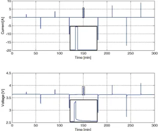
3. Pulse power tests: the data from this test is used tofit an ECM to each cell. Each pulse consists of a 10 s current followed by a 30 min rest, allowing the cell to settle such that the measured cell voltage is approximately equal to vOC. In a pulse test there are ten pulses: five charging, five discharging, at increasing magnitudes and scaled relative to the maximum current rate of the cell. The pulse test is repeated at 20%, 50%, 80% and 95% SOC to capture the impedance variation across theSOCrange. Results from an example pulse test at 50% SOC are shown inFig. 3, with a zoomed-in plot for the third charging pulse to show the typical response of the cell.
[image:6.595.42.548.707.742.2]4. EIS: The EIS test was performed with a peak current amplitude of C/20, from 100 kHz down to 10 mHz. The high frequency
Table 1
Comparison of applied and measured current.
Applied current (A) 6 12 24 0 24 12 6
Estimated net current (A) 5.9981 11.998 24.011 0.00042 24.005 12.007 6.0053
inductive region was ignored since inductance is not accounted for in the model. An example Nyquist plot of impedance for a new cell at 50% SOC is given inFig. 4a, with various frequencies annotated for clarity. Typically, the high frequency region (10e1000 Hz) is most affected by ageing[24], which means the lower frequency region of the impedance curve on the Nyquist plot will shift to the right. This can be seen in the ageing results inFig. 4b, discussed in Section3.2.2. The lowest frequency re-gion of the impedance curve corresponds to diffusion in the electrodes[25]. This region goes up to the turning point in the curveejust under 1 Hz in thefigure and the impedance at this point is used as a metric to quantify cell ageing.
3.2.2. Cycle ageing
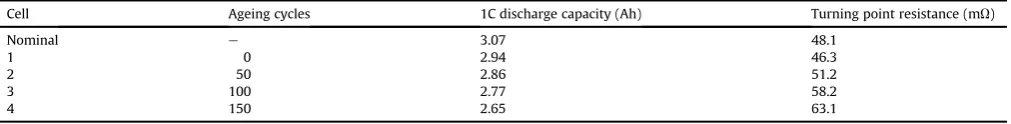
[image:7.595.134.451.68.329.2]Each ageing cycle consists of a 1C (3 A) discharge to 2.5 V fol-lowed by a constant current-constant voltage charge at C/2 (1.5 A) to 4.2 V. The cycle was chosen to age the cells quickly without overstressing the cells; the current magnitude is not at the cell's limit, but the full Depth of Discharge (DOD) ages the cells faster than a narrow DOD cycle[26]. The four cells were each aged by different amounts in order to ensure that each cell would have significantly different impedance and capacity values. The cells were aged by 0, 50, 100 and 150 cycles respectively. The two main metrics of cell ageing are impedance rise and capacity fade[8]. The results in Table 2 show that the ageing cycles cause a steady Fig. 3.Current and voltage measurements for a pulse test at 50% SOC.
[image:7.595.84.506.370.581.2]increase in resistance and decrease in capacity. The change in impedance for the cells at 50% SOC can be seen inFig. 4b. There is some increase in ohmic resistance with age, but the largest change in impedance occurs because of the growth of the semicircle at around 20 Hz. This pushes the low frequency diffusive region of the curve to the right, increasing the effective resistance of the cells as they age.
4. Model parameterisation and validation
The pulse power test data described in Section3.2.1were used to identify model parameters for each cell. A nonlinear least squares algorithm was used to estimate the vector of unknown model pa-rameters
Q
. aording to(21). This cost function aims to minimise the difference in voltage between the measured voltagevt. d the estimated voltagevbt.Q
argminXN n¼1
½vtnbvtnðt;icell;QÞ
2
Q¼RD;RP;1; CP;1…CP;nRC
(21)
A real-world test profile derived from an EV operating in an urban environment was employed to exercise the four cells con-nected in parallel and to check the accuracy of the parameter-isation. The peak current was 4C and the root mean square (RMS) current was 1.8 C. The test was initialised at 70% SOC. A 6.5% reduction in SOC over the 20 min duration of the test was observed.
Fig. 5shows the applied current for the test profile. This profile was also employed as an input to the parameterised parallel cell model. The cell currents calculated using the model were compared with the cell currents measured during the test to quantify the accuracy of the parallel cell model.
The individual ECMs were initially parameterised using data sampled at 10 Hz, the maximum rate of the cell cycler. However, the cell currents were logged using a separate data logger sampling at 100 Hz. When the parameters obtained from 10 Hz data were used for model validation, the current distribution was found to be relatively inaccurate. This is because after each change in applied current, the cell current distribution is initially dominated by the high frequency impedance of the cell. The sampling rate for pulse power tests will typically not be high enough to capture the true DC resistance and instead the ohmic resistance (RD) will be the resis-tive component of the impedance beyond the sampling frequency
[image:8.595.52.558.85.147.2][27]. FromFig. 4it can be seen that the actual DC resistance, which occurs at 631 Hz, will be much better approximated byRDwhen captured with 100 Hz data than with 10 Hz data. This means the RC pairs arefitted across the frequency spectrum and better capture the high frequency response of the cell, which improves the accu-racy of the cell current calculation.
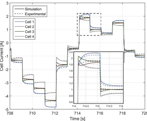
Table 3shows a comparison of the peak and RMS error in cell current and terminal voltage forfive model parameterisations. 1e3 RC pairs arefitted to the 100 Hz data, and 1e2 RC pairs arefitted to the 10 Hz data (only the 100 Hz data is parameterised with a third RC pair because of its wider bandwidth). The 2RC model using the 10 Hz data has similar accuracy to the 1RC model using the 100 Hz data, because the time constants of the models parameterised at 100 Hz are generally faster than those from the 10 Hz models. This shows that the sampling rate is important as well as model order. For current, the RMS and peak error both decrease as the number of RC pairs increases. The 3RC model, which contains the fastest time constant, is accurate to 2%, based on the RMS of the applied current. There is a similar trend with terminal voltage. A snapshot of the experimental and simulated current using 3RC pairs for the four cells is shown inFig. 6, including a zoomed-in region covering 2 s. It can be seen that for all four cells, the simulated current (solid lines) matches the measured current (dashed lines) well, even when the current distribution is changed significantly due to a step change in the applied current.
These results show that some of the most important aspects of a parallel cell unit's response occurs at high frequencies. This can be the region in which the greatest divergence in current occurs. However, a typical BMS sampling rate of 1 Hz would not capture this response, even if there were current sensors for the parallel branches. A model could estimate the current, but it would not be possible to re-parameterise the fastest RC pair components online as the cell ages.
Table 2
Summary of cell ageing results.
Cell Ageing cycles 1C discharge capacity (Ah) Turning point resistance (mU)
Nominal e 3.07 48.1
1 0 2.94 46.3
2 50 2.86 51.2
3 100 2.77 58.2
[image:8.595.43.290.530.725.2]4 150 2.65 63.1
Fig. 5.Current profile for validation drive cycle.
Table 3
Comparison of error between simulated and experimental data for various models. Sample rate 100 Hz 10 Hz
RC Pairs 1 2 3 1 2
[image:8.595.312.564.681.742.2]5. Analysis
Two main applications for electric vehicles are considered. Firstly, a hybrid electric vehicle (HEV) type drive cycle, where the overall change in SOC is low but the current profile is very dynamic and relatively large current magnitudes are expected. Secondly, a battery electric vehicle (BEV) drive cycle, in which the currents are lower but the SOC window of operation is much wider. Addition-ally, the effects of interconnection resistance and cell disconnection - two factors unique to cells connected in parallel are explored further using the validated modelling framework.
5.1. HEV application
The same current profile as the validation current (shown in
Fig. 5) was used to assess HEV applications. This was employed as the input to the parallel cell model, but with the shunt resistors removed to simulate the cells as they would be in a conventional battery pack. Two metrics are used to evaluate the cell current over the drive cycle: the peak current, and the overall charge throughput, given by (22). The peak current is scaled relative to what it would be if all cells were identical, i.e. the applied current at that time divided by the number of cells. Similarly, the charge throughput would be 25% for all of the cells if they were identical. These results are shown inTable 4. As it can be seen, cell 1 expe-riences 7% more charge throughput than cell 4, which as discussed in Ref.[8]would lead to faster ageing and higher localised tem-peratures within the system. Additionally, the SOC of cell was 4 consistently higher than the others, implying that for a HEV type application the increase in cell resistance has a greater detrimental impact than the corresponding reduction in decrease in cell capacity.
qnorm¼100 Z
jicellj
Z
iapp
(22)
It was observed that following a step change in current, in some instances the cell currents diverge and at other times they converge. This effect has to do with the magnitude of applied current. If the applied current is low, the self-balancing nature of the cells dominates the system response. The relative difference in cell current will decrease as the cells reach the same SOC. However, this is actually at odds with the dynamics of a parallel cell system. AsFig. 4b shows, all of the aged cells have a similar high-frequency resistance with a larger difference at lower frequencies. As such, for a very short time period (in the millisecond range) after a step current is applied the cell currents will be similar. After a longer period of time the lower frequency response of the cells is excited and a greater difference in resistance is exhibited by each cell, causing the cell currents to diverge. When the magnitude of the applied current is larger, the self-balancing effect driven by the voltage difference is small relative to the cells' natural response to current excitation and the currents diverge. This means that aged cells within a parallel unit will see high currents like the newer cells, but only for a short period of time.
These effects can be observed in the experimental current data shown inFig. 6. From 708 to 712 s, there are four increases in applied current magnitude, and each time the cell currents diverge after the step change. From 712 to 714 s there are two reductions in cell current and the cells self-balance following the voltage differ-ences driven by the previously large currents. Note also the current response at 716e717 s where the applied current magnitude is quite low. In this case the convergent and divergent responses largely cancel each other out resulting in a consistent current over the 1 s period.
5.2. BEV application
[image:9.595.36.280.65.266.2]Compared to a HEV, a BEV is more likely to operate in a much wider SOC window, and be subject to less dynamic loading. To consider this, a full discharge and CC-CV charge cycle is modelled, with charging and discharging currents both at 12 A (1C). For constant voltage charging, a means of translating cell voltage into applied current is required. Rather than creating a feedback system to control the input current, the current controller is assumed to be ideal in that it provides a current such that the cell is always at the requested voltage. In this instance, the applied current is calculated by rearranging the output of Eq.(17)to form(23), wherevappis the requested cell voltage. The peak current and charge throughput metrics are given inTable 5. The current fluctuations over the whole DOD mean that all of the cells experience a significantly higher peak current than if the cells were identical. In particular, cell 4, the most aged cell, sees over twice the nominal current at the end of the discharge. Despite this, the charge throughput results are more similar than for those recorded for the HEV case, because there is a greater opportunity for self-balancing during the load-cycle.
[image:9.595.302.380.73.113.2]Fig. 6.Comparison of simulated and experimental currents for the validation test profile.
Table 4
HEV drive cycle simulation results for current and charge throughput. Cell Peak current (%) Charge throughput (%)
1 114.4 28.6
2 99.5 25.1
3 101.1 25.5
[image:9.595.33.283.689.742.2]4 91.5 21.9
Table 5
Discharge-charge drive cycle simulation results for current and charge throughput. Cell Peak current (%) Charge throughput (%)
1 149.2 26.3
2 112.0 25.6
3 147.5 24.8
[image:9.595.302.553.689.742.2]i1¼D01 vappC0
x (23)
While the current is lower magnitude and less dynamic than the HEV drive cycle, the wide SOC range gives greater opportunity for differences in vOC and SOC. Fig. 7a shows the experimentally measured cell currents during a 1C discharge. There is a substantial change in current distribution after 2800 s, as the cells enter the low SOC region. By the end of discharge, the most aged cell (cell 4) is undergoing the largest current, and the least aged cell (cell 1) is undergoing the smallest current. This is at odds with the typically expected current distribution. This phenomenon has been previ-ously reported in Refs.[13], where the authors attributed it to the increase in resistance that occurs at low SOCs. Less aged cells, which have previously undergone more current, will be at a lower SOC (although this in itself depends on their relative capacities) and so eventually their impedance will increase beyond the impedance of the more aged cells. This causes the more aged cells to see larger currents towards the end of the discharge. In addition to this, the VOCs of some cell chemistries decreases more significantly at low SOCs. This means that during discharge the VOCof lower SOC cells will be significantly closer to the terminal voltage and so less cur-rent is able toflow. Eq.(24)represents(1)re-arranged to solve for current, with RC pair voltages removed for simplicity. From this it can be seen that the resistance rise and lower vOCboth work to reduce the current through low SOC cells.
icell¼vtRvOC
D (24)
This all means that the performance of the cells is quite dynamic and varied and it is an oversimplification to assume that the current distribution isfixed and the most aged cell will always undergo the smallest current. The variation will be dependent on cell charac-teristics such as the vOC-SOC curve and how the cell's impedance varies with SOC. Additionally, as highlighted here, the overall per-formance of the parallel cell unit will be application dependent and relate to the magnitude, duration and frequency content of the electrical load current. For example, a HEV battery pack is typically maintained within a narrow SOC window centred about 50% SOC. This means it won't undergo the same current switching discussed as a BEV may do.
The cell's temperature change during a discharge is known to be a function of impedance and current [28]. Fig. 7b shows the
measured cell surface temperature corresponding to the discharge profile inFig. 7a. The ambient temperature was regulated at 25C, and the temperatures were measured using T-type thermocouples attached to each cell, positioned midway along its length. Atfirst, cell 1 undergoes the greatest temperature rise due to the respective large cell current. However, after 1000 s the temperature of cell 4 surpasses that of cell 1. By this point there is not as much difference in cell currents, and so the higher impedance of cell 4 causes greater heat generation despite the lower current. The temperature of cell 2 is consistently the lowest of all of the cells because it has a relatively low impedance without seeing the large currents experienced by cell 1.
5.3. Cell connections
A battery pack containing cells in parallel requires many cell interconnections to ensure all cells are in the current path. Typi-cally, cells are grouped into parallel units, and each unit is then connected in series. Two potential issues relating to the connec-tions within a parallel unit are considered: the connection resis-tance not being negligible, and the failure of a connection. Both of these have implications for the entire battery pack performance as well as for the current distribution within the parallel unit.
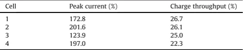
For the simulation results and verification of the modelling framework presented, it has been assumed that there is no addi-tional resistance between each cell. For the experimental work, the wires from each cell were all connected to a common pair of ter-minals, so there was no unique connection between adjacent cells. However, often cells in parallel are connected in a‘ladder’format, such as that presented inFig. 1b, in which thefirst cell is connected to the terminals, and the other cells are connected to each other. Ideally, the connection resistance (Rcin theFig. 1b) would be zero, or at least negligible relative to cell impedance. However, if there is a poor connection it can have a significant impact on the pack as a whole [15]. The simulation study presented in Section 5.2 was repeated withRcset to 5 m
U
, and the results are show inTable 6. The overall effect of this inclusion is to decrease the electrical load on the cells furthest from the terminals, as interconnection resis-tance accumulates. As a result, the charge throughput for cell 4 was a further 1% lower than in Section5.2, but higher for the other cells. Similarly, the increased differences in effective impedance caused greaterfluctuations in current, notably for three of the cells seeing higher peak currents. For the parallel system as a whole there was 1.34% less charge throughput, because the increased effective impedance of the parallel stack means that the minimum and maximum cell voltage limits are reached earlier when the cells are under electrical load. [image:10.595.46.292.64.252.2]If a cell disconnects from the parallel unit or malfunctions resulting in an internal open-circuit condition, which can occur through excessive vibration or shock loading[29], the remaining cells will continue to function. However, there will be a shorter discharge time because there is less total energy available and a greater effective parallel unit impedance that will further decrease energy availability and reduce power capability. This was simulated during a 1C discharge, where cell 2 was effectively disconnected Fig. 7.Experimental cell currents (a) and temperatures (b) for a 1C discharge of aged
cells connected in parallel.
Table 6
Simulation results for current and charge throughput, with interconnection resistance.
Cell Peak current (%) Charge throughput (%)
1 172.8 26.7
2 201.6 26.1
3 123.9 25.0
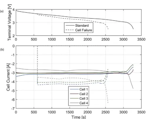
[image:10.595.312.563.690.742.2]after 600 s by setting its resistance to 10 k
U
. The results are sum-marised inFig. 8, where solid lines represent the standard case, and the dashed lines represent the failure case.Fig. 8a shows the par-allel unit terminal voltage, andFig. 8b shows the four cell currents in both cases. There is an instantaneous drop in terminal voltage and increase in the magnitude of the remaining cell currents, and the parallel unit reaches the lower cut-off voltage 703 s earlier than if there had been no disconnection. In this case, there is a 55 mV drop in terminal voltage once the cell has disconnected, and an algorithm could be created to detect a sudden change in voltage without a corresponding change in current. However, if discon-nection occurs under low, zero or a very dynamic load the disconnection may not be detected. The remaining cells, under load, are more likely to be taken outside of their intended window of operation for temperature and current.6. Conclusions and future work
The primary results from the experimental and simulation work presented highlights that cells with different impedances and ca-pacities connected in parallel do not behave in a uniform manner and can experience significantly different currents. The distribution of cell current is shown to be a complex function of impedance, including the high frequency aspects typically ignored for single cell models, and the difference in SOC between cells. As a con-ventional BMS design does not monitor current within parallel units, some cells may be taken above their intended operating current, or be aged more quickly due to increased charge throughput and ohmic heat generationeshortening the lifespan of the overall battery pack. Similarly, a cell losing electrical contact with the battery pack could result in poor SOC estimation, leading to the driver being misled about the available range of the vehicle. A typical HEV drive cycle does not appear to cause a significant amount of SOC variation between cells in parallel due to its dy-namic nature. However, for a BEV drive cycle that employs lower currents over a much larger DOD, cells can enter regions of nonlinearity. This causes significant variation and lead to cases where higher impedance cells can actually undergo larger currents. For both HEV and BEV applications, variations in current between different parallel connections of cells can cause uneven heat gen-eration within a pack, which may require a higher degree of ther-mal management.
The new framework for parallel cell modelling and the validated instantiation of a simulation model for four 18650 cells connected electrically in parallel can be used to analyse the combined effect of cell-to-cell parameter variations and different usage profiles for both BEVs and HEVs applications. The same methodology may be further employed to simulate larger energy storage systems in which individual cell models are parameterised through a statis-tical process relative to a nominal cell to explore the impact that variations in cell characteristics, thermal and interconnection properties have on complete battery pack performance and ex-pected life. Second-life applications are currently being explored, where cells at different SOHs are connected together for grid storage applications[30]. Using the parallel cell models developed here will allow for detailed simulations of the expected variations in current that may occur under load. This would further improve the design of the storage system and help ensure reliable operation. One considerable advantage of the proposed new model is that the parallel ECM is in the same form as a single cell model in which the causality between the terminal voltage and input current is main-tained. This means that state observers and other control engi-neering techniques can now be developed for parallel units in the same way as they currently are for single cells or for cells connected electrically in series. This has the potential to make parallelized battery packs more reliable by improving fault detection methods. Another important aspect of cells in parallel is how they age. The results of this work show cells at a lower SOH typically see lower currents than other cells. This implies that they should age slower than the other cells, and so it is expected that gradually the SOHs of the cells within the parallel unit will converge. Ageing testing and analysis is currently being performed using the same cells to evaluate the impact of connecting cells in parallel on ageing and will be reported in a subsequent publication.
Acknowledgements
The research presented within this paper is supported by the Engineering and Physical Science Research Council (EPSRCeEP/ I01585X/1) through the Engineering Doctoral Centre in High Value, Low Environmental Impact Manufacturing. The research was un-dertaken in collaboration with the WMG Centre High Value Manufacturing Catapult (funded by Innovate UK) in collaboration with Jaguar Land Rover. Details of additional underlying data in support of this paper and how interested researchers may be able to access it can be found here:http://wrap.warwick.ac.uk/75955/.
Nomenclature
Symbols
C C rate of applied current (current scaled by capacity) h1 C0 Effective charge capacitance of cell F
Cp Polarisation capacitance of cell F icell n Cell current for cellnA
in nth loop current in parallel cell mesh A Q Cell charge capacity Ah
Rc Connection resistance between two parallel cells
U
RD DC (ohmic) resistance of cellU
Rp Polarisation resistance of cell
U
SOC State of charge of cell % SOH State of health of cell %vapp Applied terminal voltage during constant voltage charging V
[image:11.595.35.283.60.262.2]References
[1] X. Gong, R. Xiong, C.C. Mi, Study of the characteristics of battery packs in electric vehicles with parallel-connected lithium-ion battery cells, in: Applied Power Electronics Conference and Exposition (APEC), 2014 Twenty-Ninth Annual IEEE, 2014, pp. 3218e3224, http://dx.doi.org/10.1109/ APEC.2014.6803766.
[2] X. Zhang, C. Mi, Management of energy storage systems in EV, HEV and PHEV, Veh. Power Manag. (2011) 259e286, http://dx.doi.org/10.1007/978-0-85729-736-5_8. Springer London.
[3] U.D. of Energy, Advanced Vehicle TestingeBeginning-of-Test Battery Testing Results, 2011, pp. 1e5.http://www1.eere.energy.gov/vehiclesandfuels/avta/ pdfs/fsev/battery_leaf_0356.pdf(accessed 10.22.14).
[4] J. Gallardo-Lozano, E. Romero-Cadaval, M.I. Milanes-Montero, M.A. Guerrero-Martinez, Battery equalization active methods, J. Power Sources 246 (2014) 934e949.http://dx.doi.org/10.1016/j.jpowsour.2013.08.026.
[5] Z. Zhang, P. Ramadass, Lithium-Ion battery systems and technology, in: R.J. Brodd (Ed.), Batteries for Sustainability, Springer, New York, 2013, pp. 319e357,http://dx.doi.org/10.1007/978-1-4614-5791-6_10.
[6] L. Zhong, C. Zhang, Y. He, Z. Chen, A method for the estimation of the battery pack state of charge based on in-pack cells uniformity analysis, Appl. Energy 113 (2014) 558e564.http://dx.doi.org/10.1016/j.apenergy.2013.08.008. [7] L. Lu, X. Han, J. Li, J. Hua, M. Ouyang, A review on the key issues for lithium-ion
battery management in electric vehicles, J. Power Sources 226 (2013) 272e288.http://dx.doi.org/10.1016/j.jpowsour.2012.10.060.
[8] A. Barre, B. Deguilhem, S. Grolleau, M. Gerard, F. Suard, D. Riu, A review on lithium-ion battery ageing mechanisms and estimations for automotive ap-plications, J. Power Sources 241 (2013) 680e689.http://dx.doi.org/10.1016/j. jpowsour.2013.05.040.
[9] K. Maher, R. Yazami, A study of lithium ion batteries cycle aging by thermo-dynamics techniques, J. Power Sources 247 (2014) 527e533,http://dx.doi.org/ 10.1016/j.jpowsour.2013.08.053.
[10] B. Wu, V. Yufit, M. Marinescu, G.J. Offer, R.F. Martinez-Botas, N.P. Brandon, Coupled thermaleelectrochemical modelling of uneven heat generation in lithium-ion battery packs, J. Power Sources 243 (2013) 544e554.http://dx. doi.org/10.1016/j.jpowsour.2013.05.164.
[11] K. Mueller, D. Tittel, L. Graube, Z. Sun, F. Luo, Optimizing BMS operating strategy based on precise SOH determination of lithium ion battery cells, in: Proceedings of the FISITA 2012 World Automotive Congress, Springer Berlin Heidelberg, 2013, pp. 807e819, http://dx.doi.org/10.1007/978-3-642-33741-3_9.
[12] X. Hu, J. Jiang, D. Cao, B. Egardt, Battery health prognosis for electric vehicles using sample entropy and sparse bayesian predictive modeling, Industrial Electron. IEEE Trans. PP (2015) 1,http://dx.doi.org/10.1109/TIE.2015.2461523. [13] R. Gogoana, M.B. Pinson, M.Z. Bazant, S.E. Sarma, Internal resistance matching for parallel-connected lithium-ion cells and impacts on battery pack cycle life, J. Power Sources. 252 (n.d.). doi:http://dx.doi.org/10.1016/j.jpowsour.2013.11. 101.
[14] L. Wang, Y. Cheng, X. Zhao, A LiFePO4 battery pack capacity estimation approach considering in-parallel cell safety in electric vehicles, Appl. Energy 142 (2015) 293e302,http://dx.doi.org/10.1016/j.apenergy.2014.12.081. [15] G.J. Offer, V. Yufit, D.A. Howey, B. Wu, N.P. Brandon, Module design and fault
diagnosis in electric vehicle batteries, J. Power Sources 206 (2012) 383e392.
http://dx.doi.org/10.1016/j.jpowsour.2012.01.087.
[16] J. Kim, B.H. Cho, Screening process-based modeling of the multi-cell battery
string in series and parallel connections for high accuracy state-of-charge estimation, Energy 57 (2013) 581e599. http://dx.doi.org/10.1016/j.energy. 2013.04.050.
[17] T. Baumh€ofer, M. Brühl, S. Rothgang, D.U. Sauer, Production caused variation in capacity aging trend and correlation to initial cell performance, J. Power Sources 247 (2014) 332e338.http://dx.doi.org/10.1016/j.jpowsour.2013.08. 108.
[18] X. Hu, S. Li, H. Peng, A comparative study of equivalent circuit models for Li-ion batteries, J. Power Sources 198 (2012) 359e367, http://dx.doi.org/ 10.1016/j.jpowsour.2011.10.013.
[19] A. Seaman, T.-S. Dao, J. McPhee, A survey of mathematics-based equivalent-circuit and electrochemical battery models for hybrid and electric vehicle simulation, J. Power Sources 256 (2014) 410e423,http://dx.doi.org/10.1016/ j.jpowsour.2014.01.057.
[20] A. Jossen, Fundamentals of battery dynamics, J. Power Sources 154 (2006) 530e538.http://dx.doi.org/10.1016/j.jpowsour.2005.10.041.
[21] M. Dubarry, N. Vuillaume, B.Y. Liaw, Origins and accommodation of cell var-iations in Li-ion battery pack modeling, Int. J. Energy Res. 34 (2010) 216e231,
http://dx.doi.org/10.1002/er.1668.
[22] G.L. Plett, Extended Kalmanfiltering for battery management systems of LiPB-based HEV battery packs: part 2. Modeling and identification, J. Power Sources 134 (2004) 277e292.http://dx.doi.org/10.1016/j.jpowsour.2004.02.031. [23] A. Farmann, W. Waag, A. Marongiu, D.U. Sauer, Critical review of on-board
capacity estimation techniques for lithium-ion batteries in electric and hybrid electric vehicles, J. Power Sources 281 (2015) 114e130, http:// dx.doi.org/10.1016/j.jpowsour.2015.01.129.
[24] W. Waag, S. K€abitz, D.U. Sauer, Experimental investigation of the lithium-ion battery impedance characteristic at various conditions and aging states and its influence on the application, Appl. Energy 102 (2013) 885e897.http://dx.doi. org/10.1016/j.apenergy.2012.09.030.
[25] D. Andre, M. Meiler, K. Steiner, C. Wimmer, T. Soczka-Guth, D.U. Sauer, Characterization of high-power lithium-ion batteries by electrochemical impedance spectroscopy. I. Experimental investigation, J. Power Sources 196 (2011) 5334e5341.http://dx.doi.org/10.1016/j.jpowsour.2010.12.102. [26] N. Omar, M.A. Monem, Y. Firouz, J. Salminen, J. Smekens, O. Hegazy, et al.,
Lithium iron phosphate based batteryeAssessment of the aging parameters and development of cycle life model, Appl. Energy 113 (2014) 1575e1585.
http://dx.doi.org/10.1016/j.apenergy.2013.09.003.
[27] C. Fleischer, W. Waag, H.-M. Heyn, D.U. Sauer, On-line adaptive battery impedance parameter and state estimation considering physical principles in reduced order equivalent circuit battery models part 2 parameter and state estimation, J. Power Sources (2014), http://dx.doi.org/10.1016/ j.jpowsour.2014.03.046.
[28] M. Debert, G. Colin, G. Bloch, Y. Chamaillard, An observer looks at the cell temperature in automotive battery packs, Control Eng. Pract. 21 (2013) 1035e1042.http://dx.doi.org/10.1016/j.conengprac.2013.03.001.
[29] M.A. Roscher, R.M. Kuhn, H. D€oring, Error detection for PHEV, BEV and sta-tionary battery systems, Control Eng. Pract. 21 (2013) 1481e1487.http://dx. doi.org/10.1016/j.conengprac.2013.07.003.