Dynamic properties of condensing particle systems

(1)

warwick.ac.uk/lib-publications

A Thesis Submitted for the Degree of PhD at the University of Warwick

Permanent WRAP URL:

http://wrap.warwick.ac.uk/91746

Copyright and reuse:

This thesis is made available online and is protected by original copyright.

Please scroll down to view the document itself.

Please refer to the repository record for this item for information to help you to cite it.

Our policy information is available from the repository home page.

(2)

Dynamic Properties of Condensing Particle Systems

by

Thomas Keith Rafferty

Thesis

Submitted to the University of Warwick

for the degree of

Doctor of Philosophy

Mathematics Institute and Centre for Complexity Science

(3)

Acknowledgments

Firstly, I would like to express my sincere gratitude to my supervisors, Stefan

Grosskinsky and Paul Chleboun, for their constant support and guidance. Their

knowledge and advice have helped me to keep on track and tackle the more

interest-ing problems in the field of stochastic particle systems. I am especially grateful to

Paul Chleboun and Andrea Pizzoferrato for making themselves available for many

post lunch coffee discussions of the various topics studied in and around this thesis.

I would also like to express my thanks to all the members of the DTC and

CDT for making the past 4 years so enjoyable and making the department such a

relaxed environment to do research in. Additional thanks go to all those people

out-side the department with whom I have had the opportunity to discuss my research,

their feedback has been invaluable in the construction of this thesis.

Finally, I would like express my thanks to my family. I am also especially

grateful to Merve Alanyalı for her enthusiasm, interest and support throughout this

(7)

Declarations

This work has been composed by myself and has not been submitted for any other

degree of professional qualification.

• The work done in Chapters 3 and 4 has been submitted to Annales de l’Institut

Henri Poincar´e and is under the third round of reviews.

• Work done in Chapters 5 and 6 will be submitted for publication.

• The construction of the growth process given in Appendix A.2 was first given

(8)

Abstract

Condensation transitions are observed in many physical and social systems, ranging from Bose-Einstein condensation to traffic jams on the motorway. The un-derstanding of the critical phenomena prevalent in these systems presents many interesting mathematical challenges. We are interested in understanding the vari-ous definitions of condensation which are suitable in the field of stochastic particle systems and how they are related. Furthermore, we are also interested in dynamic properties of processes that undergo the condensation transition, such as typical convergence time scales and monotonicity properties.

Condensation can be defined in many different ways; considering the thermo-dynamic limit, a weak law of large numbers for the maximum occupation number, and an infinite particle limit on fixed finite lattices. For the latter definition, and processes that exhibit a family of stationary product measures, we prove an equiva-lent characterisation in terms of sub-exponential distributions generalising previous known results.

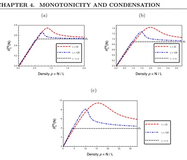
All known examples of condensing processes that exhibit homogeneous sta-tionary product measures are non-monotone, i.e. the dynamics do not preserve a partial ordering of the state space. This non-monotonicity is typically characterised by an overshoot of the canonical current, which on a heuristic level is related to metastability. We prove that these processes with a finite critical density are nec-essarily non-monotone confirming a previous conjecture. If the critical density is infinite, condensation can still occur on finite lattices. We present partial evidence that there also exist monotone condensing processes.

(9)

Introduction

Condensation is ubiquitous in nature. In addition to the classical definition of vapour condensation, it has also been observed in the context of quantum mechanics. For example, first predicted by Einstein in 1924 [1] and since experimentally observed in 1995 [2] Bose-Einstein condensation occurs in a dilute gas of bosons cooled to absolute zero. Condensation can also occur in population models and most notably in Kingman’s model of the distribution of the fitness of a population undergoing selection and mutation [3]. When the rate of selection dominates the rate of muta-tion, a condensation transition occurs since a positive proportion of the population in later generations takes an optimal fitness [4]. The growth of complex networks such as the World Wide Web may also exhibit a condensation transition due to a preferential effect as new nodes (or links) aim to connect to nodes which are already popular to increase visibility, resulting in the “rich get richer” or “winner takes all” phenomena [5]. Condensation and the “rich get richer” phenomena have also been observed in simple economic models of the distribution of wealth in a population [6]. Simple particle models of traffic dynamics with applications to the transport of mass in cells and on the road network, known as stochastic particle systems, have been shown to condense/jam due to local interactions [7] or system defects [8, 9]. In this thesis, we study condensation in stochastic particle systems through system defects or particle interactions.

(10)

also represent a natural extension to the theory of Markov processes. Typically, the global evolution of stochastic particle systems is Markovian, however, the trajecto-ries of single particles are not. This local non-Markovian behaviour is due to local interactions and leads to difficulties in calculating typical convergence time scales of the process and hydrodynamic limits, which describe the large scale dynamics of the processes [12].

Recent research has focused on understanding the dynamic properties of con-densing stochastic particle systems. An example of such a system is the zero-range process, which is a stochastic particle system without restriction on the local oc-cupation numbers and the jump rate only depends on the number of particles on the departure site. It is known that condensation occurs if the jump rate decreases sufficiently slowly with the number of particles, see for example [13, 7]. First results on the nature of the condensate in zero-range processes are discussed in [14, 15]. In the condensed phase the canonical current typically exhibits a large overshoot above its value in the thermodynamic limit [16], which leads to a metastable switch-ing (hysteresis) between a fluid and condensed phase. This switchswitch-ing phenomenon is related to a separation of time scales and therefore metastability, which has been rigorously established for a condensing zero-range process in [17] on finite lattices and in [18] for the thermodynamic limit. Before reaching stationarity the dynamics of the process in the condensed phase correspond to a coarsening process as increas-ingly large clusters appear on a decreasing number of sites [19, 20, 21]. Coarsening, hysteresis, and metastability are not only features of the zero-range process but are also found in other condensing stochastic particle systems. The inclusion process is similar to the zero-range process with the addition of an attractive component where now the jump rates depend on departure and arrival sites. Coarsening and metastability results for the condensing inclusion process have been established rig-orously in [22, 23] for finite lattices and heuristically in [24] in the thermodynamic limit.

(11)

deep connections to the spatial properties spin systems [25, 26, 27, 28]. For stochas-tic parstochas-ticle systems such as the exclusion and zero-range processes sharp bounds on the relaxation time are only known in certain cases and results typically rely on monotonicity and coupling tools. By a simple mapping, the symmetric exclusion process and the symmetric constant rate zero-range process on the one dimensional torus can be shown to be equivalent and therefore have the same relaxation time [29]. Furthermore, the relaxation time for the constant rate zero-range process on any geometry can be calculated from comparisons of the process on the complete graph [30], provided the process is reversible. In [31] a recursive method of bound-ing the relaxation time was found by a decomposition of the state space, a method which was first introduced for the Kawasaki Ising model [32] and has since been used to give crude bounds for general Markov chains [33].

The mixing time of a Markov chain characterises how fast a process ap-proaches stationarity and can exhibit highly non-trivial behaviour. An example of this is the cutoff phenomenon, where the distance stays close to its maximal value, then drops suddenly to a small value and then tends to zero exponentially fast, which is characterised by the relaxation time. The cutoff phenomenon was first discovered in card shuffling problems [34], which heuristically implies that it takes roughly 7 riffle shuffles to adequately mix a deck of 52 cards. Cutoff then allows us to restate the question of convergence from asking “how close to stationarity are we after say 106 steps?” to asking “will 7 steps suffice?” For an early review of the cutoff phenomenon in card shuffling and urn models see [35]. For stochastic particle systems establishing a cutoff is extremely difficult and results are only known for the exclusion process on various underlying geometries. For the complete graph exclusion process, a result was first obtained in the case ofnparticles and 2n sites by a comparison of the process to the Bernoulli-Laplace diffusion model [36], and has since been generalised in [37] by restating the problem as a birth-death process. Cutoff for the symmetric simple exclusion process on the one dimensional torus was established in the sequence of papers [38, 39, 40] by comparing the process to the discrete heat equation and coupling the process with dynamics of an interface first developed in [41].

(12)

(13)

Interacting Particle Systems

In this chapter, we construct the interacting particle systems which are studied in this thesis and summarise the results which are most relevant. We also introduce the key concepts and results treated in this work, such as couplings and monotonicity, and relaxation times.

The construction of interacting particle systems presented here closely follows [42, 43]. To construct couplings of interacting particle systems we follow [42, 44] and review [45]. Discussions on relaxation, mixing and hitting times largely follow [44, 46].

2.1 Markov processes, semi-groups, generators and the

master equation

Interacting particle systems are continuous time Markov processes denoted by (η(t))t≥0

with state space Ω =EΛ where Λ is a finite or countable lattice andE is a count-able set. The dynamics are typically specified by giving the (infinitesimal) rates for transitions to occur between two states in the state space.

The state space Ω =EΛof the process is the set of all possible configurations, for example the setE is given by Nfor zero-range dynamics or {0,1}for exclusion processes, which are discussed in Section 2.3. Configurations are denoted by Greek lettersη = (ηx)x∈Λ∈Ω, where ηx∈E denotes the occupation of the sitexfor each

x∈Λ. In addition, ηx(t) denotes the occupation of site x∈Λ at timet. The state

space Ω is endowed with the product topology which is metrizable, with measurable structure given by the Borelσ-algebra B.

The time evolution of the processes is given by sample paths from the canon-ical path space

(14)

2.1. MARKOV PROCESSES

Let F be the smallest σ-algebra on D[0,∞) relative to which all functions η(·)7→η(s) fors≥0 are measurable. Fort∈[0,∞), letF_tbe the smallestσ-algebra relative to which all functionsη(·)7→η(s) for 0≤s≤tare measurable. The filtered space (D[0,∞),F,Ft) serves as a generic choice for the probability space of the

process.

Definition 2.1.1. A Markov process on Ω is a collection of{_Pη :η∈Ω} of

proba-bility measures onD[0,∞) indexed by initial configurationsη∈Ωwith the following properties;

(i) Pη[ξ(·)∈D[0,∞) :ξ(0) =η] = 1for allη ∈Ω.

(ii) Eη[ξ(s+·)∈A| Fs] =Pξ(s)[A]for every η∈A and A∈ F.

(iii) The mapping η7→_P_η[A]is measurable for everyA∈ F.

For a Markov process the expectation corresponding to Pη will be denoted

byEη which is given by

Eη[A] = Z

D[0,∞)

A dPη ,

for any measurable functionA on D[0,∞) which is integrable with respect toPη.

Property (i) states that Pη is normalised on paths with initial configuration

η∈Ω. (ii) is the Markov property which ensures that the probability of some future event, conditioned on the history of the process up to some timesonly depends on the configuration at time s. Property (iii) allows us to consider the process with arbitrary initial distributionν on Ω, defined by

Pν = Z

Ω

Pην(dη) .

The dynamics of the process are specified by the rates at which transitions from η to η0 ∈ Ω denoted c(η, η0) ≥ 0, called transition rates. Intuitively the transition rates have the following meaning

Pη[η(dt) =η0] =c(η, η0)dt+o(dt) as dt&0 for η 6=η0 , (2.1)

i.e.in a small time windowdt the process transitions from η toη0 with probability approximately given byc(η, η0)dt. The transition ratec(·,·) is assumed to be a non-negative, uniformly bounded and continuous function of η and η0 in the product topology on Ω.

(15)

the state space is not necessarily compact but countable, and therefore the processes we consider are Markov chains and their constructions can be found in [42, 47]. The construction of theses processes on infinite lattices must be done on a case-by-case basis, for example [48, 49] and [50] for a zero-range process. Throughout this work, we focus on processes defined on finite state spaces with a fixed number of particles and consider their properties in the thermodynamic limit or as the particle number diverges.

We now define Markov semigroups and state the main results which show one-to-one correspondence between Markov semigroups and processes. Let C(Ω) denote the set of continuous bounded functionsf : Ω→ _R, which is regarded as a Banach space with||f||:= sup_η∈Ω|f(η)|.

Definition 2.1.2. For a given process {_P_η :η ∈Ω}, for each t ≥0 we define the operatorS(t) :C(Ω)→C(Ω)by

(S(t)f)(η) :=Eη[f(η(t))] . (2.2)

A Markov process is said to be a Feller process ifS(t)f ∈C(Ω)for every t≥0 and

f ∈C(Ω).

The properties of the linear operators{S(t), t ≥0} arising from Feller pro-cesses{Pη :η∈Ω}are given in the following proposition.

Proposition 2.1.3. Suppose {Pη : η ∈ Ω} is a Feller process on Ω. Then the

collection of linear operators{S(t) :t≥0} onC(Ω) has the following properties;

(i) S(0) =I, the identity operator onC(Ω).

(ii) The mapping t 7→ S(t)f from [0,∞) → C(Ω) is right continuous for every

f ∈C(Ω).

(iii) S(s+t)f =S(s)S(t)f for everys, t≥0 and f ∈C(Ω).

(iv) S(t)1=1 for allt≥0.

(v) S(t)f ≥0 for all non-negative f ∈C(Ω).

Proof. See, for example, [42, Proposition 1.3].

(16)

2.1. MARKOV PROCESSES

The operator S(t) determines the time evolution of functions f ∈ C(Ω), which are interpreted as observables. Markov semigroups are in one-to-one corre-spondence with Markov processes outlined in Proposition 2.1.3 and the following theorem.

Theorem 2.1.5. Suppose {S(t) : t ≥ 0} is a Markov semigroup on C(Ω). Then there exists a unique Feller Markov process {_P_η : η ∈ Ω} such that (2.2) holds for allt≥0.

Proof. See for example [42, 47]

Therefore, the semigroup provides a full representation of the Markov pro-cess, dual to the path measures{Pη :η ∈Ω}since C(Ω) is dual to the setP(Ω) of

probability measures on Ω. The expectation of observables att≥0 with respect to the initial distributionν ∈ P(Ω) is given by

Eν[f(η(t))] = Z

Ω

(S(t)f)(ξ)ν[dξ] =

Z

Ω

S(t)f dν for all f ∈C(Ω).

From property (iii) of Proposition 2.1.3 we expect {S(t) : t ≥ 0} has an exponential form characterised byS0(0), the time derivative of S(t) at zero, in the sense

S(t) = “eS0(0)t” =I+S0(0)t+o(t) withS(0) =I . (2.3)

This is made precise as follows.

Definition 2.1.6. The (infinitesimal) generator L : DL → C(Ω) for the process

{S(t) :t≥0} is given by

Lf = lim

t&0

S(t)f−f

t for allf ∈DL , (2.4)

where the domain DL⊆C(Ω) is the set of all functions for which the limit exists.

For finite state spaces, Ω,DL=C(Ω), otherwise one often has to restrict to bounded cylinder test functions [42].

Proposition 2.1.7. L as defined by (2.4)is a Markov generator, i.e.

(i) 1∈DL and L₁=1 (Conservation of probability).

(ii) For allf ∈DL and λ >0, minξ∈Ωf(ξ)≥minξ∈Ω(f−λLf)(ξ) (Positivity).

(17)

Proof. See for example [42, Proposition 2.2]

Theorem 2.1.8.(Hille-Yosida) There is a one-to-one correspondence between Markov generators and semigroups on C(Ω), given by (2.4) and

S(t)f =etLf := lim

n→∞

I− t nL

−n

f for f ∈C(Ω)and t≥0 . (2.5)

Furthermore, iff ∈DL thenS(t)f ∈DL for all t≥0, and

d

dtS(t)f =S(t)Lf =LS(t)f , (2.6)

called the forward and backward equations respectively.

Proof. See for example [42, Theorem 2.9]

Finally, for finite systems with a finite state space, the generator can be computed directly from (2.2) and the heuristic (2.1) as follows

S(dt)f =Eη[f(η(t)] = X η0_∈_Ω

f(η0)Pη[η(dt) =η0]

= X

η0_∈_Ω

c(η, η0)f(η0)dt+f(η)



1− X η0₆₌_η

c(η, η0)dt



+o(dt).

Then (2.4) implies

Lf(η) = X

η0₆₌_η

c(η, η0) f(η0)−f(η)

. (2.7)

Markov processes and semigroups are therefore characterised by the transition rates c(η, η0) between states η and η0. We use the convention that c(η, η0) = 0 for all η=η0 ∈Ω.

From the generator and semigroup definitions of finite state Markov pro-cesses, we can immediately construct the master equation as follows: Consider the indicator functions 1η : Ω → {0,1}, which are bounded and form a basis of C(Ω)

for finite Ω, defined by

1η(ξ) =  



1 ifξ =η

(18)

2.2. STATIONARY MEASURES

Letpt=µS(t) denote the distribution on Ω at time tcharacterised by

pt[f] = Z

Ω

S(t)f dν . (2.8)

Substitutingf(η) =1(η) into the forward equation (2.6) we have

d

dtpt[η] =

Z

Ω

S(t)L₁ηdν= X ξ∈Ω

pt[ξ] X ξ0_∈_Ω

c(ξ, ξ0) 1η(ξ0)−1η(ξ)

=X

ξ∈Ω

pt[ξ]c(ξ, η)−pt[η] X ξ0_∈_Ω

c(η, ξ0) , (2.9)

which is called the master equation.

2.2 Stationary measures, reversibility and ergodicity

Definition 2.2.1. A probability measure µ∈ P(Ω) is said to be stationary or in-variant if it satisfies µ(S(t)f) = µ(f) for all t≥0 and f ∈C(Ω). The measure is called reversible ifµ(f S(t)g) =µ(gS(t)f) for allf, g∈C(Ω).

Here and throughout this thesis we use the notationµ(f) =R_Ωf dµto denote the expectation off ∈C(Ω) with respect to the measure µon Ω.

It is clear that every reversible measure µis stationary (taking g≡1). The probabilistic interpretation of a stationary measureµis given by a processη(t) with initial distributionµ has the same distribution as η(t+s) for every s∈[0,∞), or formally

Pµ[η(·)∈A] =Pµ[η(t+·)∈A] for all t≥0, A∈ F .

Equivalently, using (2.8) ifp0 =µthenpt=µfor all t≥0.

Proposition 2.2.2. A measureµ∈ P(Ω)is stationary if and only if

µ(Lf) = 0 for all f ∈DL .

Furthermore, the measure µis reversible if and only if

µ(fLg) =µ(gLf) = 0 for all f, g∈DL .

Proof. See for example [42, Propisition 2.13].

(19)

Proposition 2.2.3. A measure µ on a countable state space Ω is reversible for the process with transition rates c(·,·) if and only if it fulfils the detailed balance conditions

µ[η]c(η, ξ) =µ[ξ]c(ξ, η) for all η, ξ∈Ω.

Definition 2.2.4. A Markov process with semigroup {S(t) : t ≥ 0} is ergodic if there exists a unique stationary measureπ∈ P(Ω)and

lim

t→∞pt=π for all initial distributions p0 ,

where pt is the distribution of the process at time t given by (2.8).

Definition 2.2.5. A Markov process {Pη : η ∈ Ω} is called irreducible if for all

η, η0 ∈Ω

Pη[η(t) =η0]>0 for all t≥0 .

The interpretation of an irreducible Markov process is as follows; an irre-ducible process can sample the entire state space from any initial condition. Irre-ducibility implies the uniqueness of the stationary measure and if the state space Ω is finite then the process is ergodic as outlined in the following theorem.

Theorem 2.2.6. An irreducible Markov process with finite state spaceΩis ergodic.

Proof. See for example [47]

2.3 Example processes

2.3.1 The zero-range process

The zero-range process (ZRP), introduced in [10], is a stochastic particle system on the state space ΩL =NΛ where Λ = {1, . . . , L}. A single particle at site x leaves at rate gx(ηx) and jumps to site y with probabilityp(x, y) where the dynamics are

defined by the generator

Lf(η) = X

x,y∈Λ

(20)

2.3. EXAMPLE PROCESSES

forf ∈C(ΩL). Hereηx,ydenotes the configuration after a single particle has jumped

from sitex toy and is given by

η_zx,y =

    

   

ηx−1 ifz=x

ηy+ 1 ifz=y

ηz otherwise

.

To ensure the process is non-degenerate and irreducible, the jump ratesgx(n) satisfy

gx(n) = 0 for all x ∈ Λ if and only if n= 0. The process is called homogeneous if

gx(n) =gy(n) for allx, y∈Λ andn∈Nand inhomogeneous otherwise. Throughout this thesis we study both homogeneous and inhomogeneous zero-range processes. Zero-range processes and similar models are often studied in a translation invariant setting (p(x, y) =q(|y−x|)) on a regular lattice with periodic boundary conditions. Typical choices in one dimension are symmetric and totally asymmetric transition probabilities with p(x, y) = 1₂δy,x+1 +1₂δy,x−1, p(x, y) = δy,x+1, or fully connected

transition probabilitiesp(x, y) = (1−δy,x)_L1−1, respectively.

Well studied zero-range processes include the constant rate zero-range pro-cess where gx(n) = 1 for all x ∈ Λ and n > 0, which is a system of L server

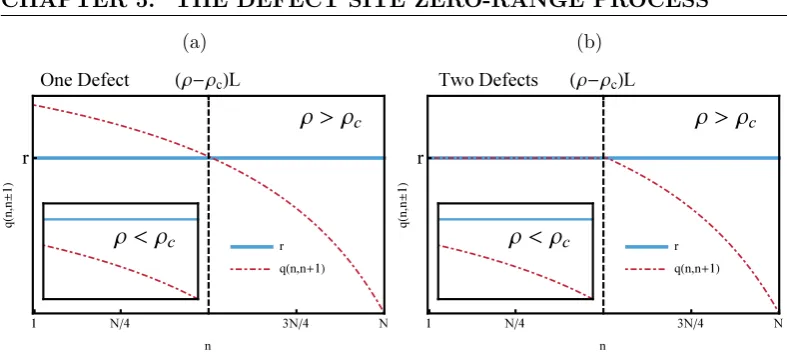
queues with mean one exponential random service times. The constant rate zero-range process can be extended to include site defects wheregx(n) =r <1 for some

x∈∆⊆Λ, which are studied in Chapter 5. Ifg(k) =kthen the zero-range process is a system of independent random walkers on Λ.

Under translation invariantp(x, y), zero-range processes defined by the gen-erator (2.10) exhibit a family of stationary product measures{ν_φL:φ∈Dφ}on ΩL,

whereφis called the fugacity and Dφ= [0, φc) or [0, φc] is the domain of the family

of measures [48]. ν_φL[·] is given by

ν_φL[η] = Y

x∈Λ

ν_φx[ηx] where νφx[n] =

wx(n)φn

zx(φ)

. (2.11)

The measures exist for all φ ∈ Dφ where φc is the determined by the radii of

convergence of the single site partition function

zx(φ) =

∞

X k=0

wx(k)φk . (2.12)

(21)

by

φx_c =

lim sup

n→∞ n

p

wx(n) −1

. (2.13)

The stationary weightswx(n) are given by

wx(n) = n Y k=1

1 gx(k)

forn >0 andwx(0) = 1 for allx∈Λ . (2.14)

The family {νφ[·] : φ ∈ Dφ} is called the grand-canonical ensemble and zx(φ) are

called the grand-canonical partition functions. The (singe site) grand-canonical densities are functions of the fugacityφ∈Dφ and are given by

ρx(φ) :=νφx(ηx) =

1 zx(φ)

∞

X n=1

nwx(n)φn . (2.15)

Since the zero-range process conserves the particle number the process is irreducible on the finite state space

ΩL,N := (

η∈ΩL : X x∈Λ

ηx =N )

. (2.16)

Therefore, the process restricted to ΩL,N is ergodic with a unique stationary measure

on ΩL,N given by

πL,N[·] :=νφL

·

η ∈Ω_L,N

. (2.17)

The family{πL,N :N ∈N}is called the canonical ensemble and these measures are independent of the fugacityφ. The measureπL,N[·] can be easily shown to have the

mass function

πL,N[η] =

1 ZL,N

Y x∈Λ

wx(ηx)1(η∈ΩL,N), (2.18)

where canonical partition function is given by

ZL,N = X η∈ΩL,N

Y x∈Λ

(22)

2.3. EXAMPLE PROCESSES

2.3.2 The misanthrope process

Misanthrope processes are generalisations of zero-range processes, where the jump rate now depends on the exit and entry sites, and are defined by the generator

Lf(η) = X

x,y∈Λ

r(ηx, ηy)p(x, y) (f(ηx,y)−f(η)) , (2.20)

forf ∈C(ΩL). Again, the configurationηx,y∈ΩLdenotes the configuration after a

single particle jumps from sitextoy∈ΩL. To ensure the process is non-degenerate

the jump rater(n, m) = 0 for allm≥0 if and only ifn= 0, andr(n, m)>0 for all n >0 and m≥0.

Misanthrope processes include many well-known examples of interacting par-ticle systems, such as zero-range processes [10], the inclusion process [51, 52], and the explosive condensation model [53]. It is known [11, 54] that misanthrope processes with translation invariant dynamics p(x, y) = q(x−y) exhibit stationary product measures of the form (2.11) if and only if the rates fulfil

r(n, m) r(m+ 1, n−1) =

r(n,0)r(1, m)

r(m+ 1,0)r(1, n−1) for all n≥1, m≥0, (2.21)

and, in addition, either

 



q(z) =q(−z) for all z∈Λ or,

r(n, m)−r(m, n) =r(n,0)−r(m,0) for all n, m≥0 .

(2.22)

The corresponding stationary weights satisfy

w(k+ 1) w(k) =

w(1) w(0)

r(1, k)

r(k+ 1,0) and w(n) =

n Y k=1

r(1, k−1)

r(k,0) . (2.23)

In [45] generalised misanthrope processes have been introduced where more than one particle is allowed to jump simultaneously. They are defined via transi-tionsη → η+n(δy −δx) for n∈ {0, . . . , ηx} at rate Γnηx,ηy(y−x) and the authors give necessary and sufficient conditions on the jump rates for the processes to be monotone.

2.3.3 Generalised zero-range processes

(23)

a stochastic particle system on the state space ΩL=NΛ defined by the generator

LgZRP_{f(η) =} X x,y∈Λ

ηx

X k=1

αk(ηx)p(x, y) f(ηx→(k)y)−f(η)

. (2.24)

Here ηx→(k)y _∈ _Ω

L is the configuration after k particles have jumped from x to

y∈Λ. The jump rates αk(n) satisfy αk(n) = 0 if k > n, and we use the convention

that empty summations are zero. We consider translation invariant p(x, y) on a finite lattice Λ = {1, . . . , L} with periodic boundary conditions and we also note that the process preserves particle numberP

xηx =N.

It is known [55, 54] that these processes exhibit stationary product measures if and only if the jump rates have the explicit form

αk(n) =g(k)

h(n−k)

h(n) , (2.25)

whereg, h:N→[0,∞) are arbitrary non-negative functions withhstrictly positive. The stationary weights are then given byw(n) =h(n).

2.4 Monotonicity and couplings

In this section, we will review the relevant results on monotone (attractive) inter-acting particle systems and give details on how to construct coupling which preserve a partial order of the state space.

We use the natural partial order on the state space ΩL=NΛ given byη≤ζ ifηx ≤ζx for all x∈Λ. A function f : ΩL →Ris said to be increasing if and only ifη ≤ζ implies f(η)≤f(ζ). Two measures µ1, µ2 on Ω are stochastically ordered

(monotone) with µ1 ≤ µ2, if for all increasing functions f : ΩL → R we have for expectationsµ1(f)≤µ2(f).

A stochastic particle system on ΩLwith generatorLand semi-group (S(t) =

etL :t≥0) is called monotone (attractive) if it preserves stochastic order in time, i.e.

µ1 ≤µ2 =⇒ µ1S(t)≤µ2S(t) for all t≥0 ,

which is equivalent to

(24)

2.4. MONOTONICITY AND COUPLINGS

Utilising the Hille-Yosida Theorem 2.1.8 and the definition of the generator (2.4) we see that the process is monotone if and only if

Lf(η)≤ Lf(ξ) , (2.27)

for all η ≤ ξ and all f ∈ C(ΩL) increasing such that f(η) = f(ξ). The condition

f(η) =f(ξ) is necessary since for the following to hold

Lf(η) = lim

t&0

S(t)f(η)−f(η) t ≤limt&0

S(t)f(ξ)−f(ξ)

t =Lf(ξ) , (2.28)

we needf(η)≥f(ξ), however, f is increasing and η≤ξ implies the equality. Coupling techniques for monotone processes are important tools to derive rigorous results on the large scale dynamics of such systems such as hydrodynamic limits [45]. Let (η(t))t≥0be an interacting particle system on ΩL. A Markov coupling

of (η(t))t≥0 with itself is a processes (ξ(t), ζ(t))t≥0 on ΩL ×ΩL such that each

marginal ξ(t) and ζ(t) is distributed as the original process (η(t))t≥0, i.e.if we

observe one of the processes without observing the other, the process behaves as it is originally constructed.

The link between stochastic monotonicity and couplings is given by Strassen’s theorem [56]:

Theorem 2.4.1. (Strassen) For probability measures µ1, µ2 on a common state

spaceΩL, µ1≤µ2 if and only if there exists a couplingµon the product state space

ΩL×ΩL such that

µ({η = (η1, η2) :η1 ≤η2}) = 1 ,

i.e. the probability of observing the partial order is 1.

Strassen’s theorem has the natural extension to couplings of stochastic pro-cesses and monotone propro-cesses.

2.4.1 Constructing a coupling for the zero-range process

In Chapter 5, we rely on known results of monotone zero-range process, therefore, here we include here a detailed construction of a coupling for the ZRP. Furthermore, understanding the construction of a coupled process is also necessary for results obtained in Chapter 4 on generalised zero-range and misanthrope processes.

Let (ξ(t))t≥0 and (ζ(t))t≥0 be two zero-range processes defined via the same

generator (2.10) such that their initial conditions satisfyξ ∈ΩL,N andζ ∈ΩL,N+1.

(25)

[image:25.595.209.435.130.267.2]

Figure 2.1: Example configuration of the coupled dynamics. Theξprocess is shown in red and the second class particle is shown in blue. The jump rates are defined according to equation (2.29) and it is clear that the coupling can only be constructed for increasing jump ratesgx(·) as we needgx(m)−gx(n)≥0 for allx∈Λ andm≥n.

(ΩL,N,ΩL,N+1) between the processes ξ(t) and ζ(t) such that, ξ(t) =η(t) +δy for

somey∈Λ, i.e.there is an extra particle in the ζ(t) process at site y, often called a second class particle. The coupling is constructed via the following rules called a basic coupling

1. The marginals of the coupled process are two zero-range processes withN and N+ 1 particles respectively and each are defined by the generator (2.10). As a consequence, when the process has converged to its stationary measure for the joint process this is a coupling of the measuresπL,N and πL,N+1 [48].

2. Particles move together as much as possible.

Ifgx(n) is non-decreasing for eachx∈Λ the coupled process behaves via the

follow-ing transition rates, which is illustrated in Figure 2.1; for the site with the second class particle

ξy =n+ 1

ηy =n o

gy(ξy)−gy(ηy) −−−−−−−−−→

n ξ_y =n

ηy =n

ξy =n+ 1

ηy =n

o _g

y(ηy) −−−−−−−−→

n ξ_y =n

ηy =n−1

, (2.29)

and for the remaining sites, both processes jump at rate gx(ηx) =gy(ξx).

(26)

2.5. MIXING, HITTING, AND RELAXATION TIMES

ΩL×ΩLis given by

Lf(ξ, ζ) = X

x,y ξx≤ζx

gx(ξx)p(x, y) (f(ξx,y, ζx,y)−f(ξ, ζ))

+ X

x,y ξx≤ζx

(gx(ζx)−gx(ξx))p(x, y) (f(ξ, ζx,y)−f(ξ, ζ))

+ X

x,y ζx≤ξx

gx(ζx)p(x, y) (f(ξx,y, ζx,y)−f(ξ, ζ))

+ X

x,y ζx≤ξx

(gx(ξx)−gx(ζx))p(x, y) (f(ξx,y, ζ)−f(ξ, ζ)) . (2.30)

For the coupling constructed in (2.29) and (2.30) to exist, the jump rate gx(n) has to be non-decreasing.

Theorem 2.4.2. The zero-range process on ΩL = NΛ defined by the generator (2.10) is monotone if and only if the jump rates satisfy gx(m)≥gx(n) for all m≥

n∈_N and x∈Λ.

Proof. ( ⇐= ) The condition gx(m) ≥ gx(n) for all m ≥n ∈N and x ∈Λ implies (2.30) is a generator of a Markov process with non-negative rates. By substitut-ing the functions f(ξ, ζ) = f1(ξ) and f(ξ, ζ) = f2(ζ) into (2.30) it is clear that

the marginals are zero-range processes with the generator (2.10). Therefore, by Strassen’s theorem the ZRP with non-decreasing jump rates is monotone.

( =⇒ ) Consider the increasing test function f(η) = ηy and two

config-urations η = nδx and ξ = mδx such that x 6= y, m ≥ n, and p(x, y) > 0.

Clearly η ≤ξ and assuming the process is monotone the inequality (2.27) implies gx(n)p(x, y)≤gx(m)p(x, y). Since the choice of x, ywere arbitrary and p(x, y)>0,

we have gx(n) ≤ gx(m) for all m ≥ n and x ∈ Λ, which completes the proof of

Theorem 2.4.2.

2.5 Mixing, hitting, and relaxation times

(27)

mea-sureπ on Ω andf, g ∈C(Ω) the inner product is given by

hf, gi_π =X

η∈Ω

π[η]f(η)g(η) ,

and

||f||₂_,π=



 X η∈Ω

π[η]f(η)2





1/2

.

2.5.1 The relaxation time and the spectral gap

The relaxation time of an ergodic Markov process characterises the exponential rate of convergence to the stationary measure. For reversible processes on a countable state space, the relaxation time is given by the reciprocal of the smallest non-zero eigenvalue of−L, called the spectral gap, where L is the generator of the process.

For a Markov process (η(t))t≥0 with generatorL on Ω with stationary

mea-sureπ, the Dirichlet form is given by

DL(f) =hf,−Lfiπ =− X η∈Ω

π[η]f(η)Lf(η) ,

forf ∈ C(Ω). For a reversible process with generator (2.7) the Dirichlet form can be rewritten as

DL(f) = 1 2

X η,ξ

π[η]c(η, ξ) (f(ξ)−f(η))2 . (2.31)

Furthermore, it is easy to show [46, Lemma 2.1.2]

d

dt||S(t)f||

2

2,π =−DL(S(t)f).

Let Varπ(f) denote the variance of a function f : Ω → R with respect to the measure π then the spectral gap and relaxation time are defined by the Rayleigh-Ritz principle as follows.

Definition 2.5.1. The spectral gap λL of the generator L on Ω is given by the variational principle

λL= inf

f _D

L(f) Varπ(f)

: Varπ(f)6= 0

, (2.32)

and the relaxation time is given by the inverse spectral gapT_Lrel:= _λ1

(28)

For a reversible process the valueλLis then the difference between the small-est eigenvalues of the generator−L.

Proposition 2.5.2. Let (η(t))t≥0 be an irreducible Markov process with stationary

measure π on the state space Ω then λL is the optimal constant appearing in the inequality

V arπ(S(t)f)≤e−2λLtV arπ(f) (2.33)

Proof. See for example [46, Lemma 2.1.4].

From Proposition 2.5.2, we see that the inverse spectral gap gives the char-acteristic time scale of the contraction of the variance of the kernel S(t) towards stationarity, whereS(t)f(η)→π(f) for allη ∈Ω.

2.5.2 Mixing times

The mixing time of a Markov process is another measure of how far the process is from the stationary distribution, which are measured by the total variation distance. The total variation distance between two measuresµand ν on Ω is given by

||µ−ν||T V = max

A∈Ω|µ[A]−ν[A]|. (2.34)

By Proposition 4.2 of [44] the total variation distance can be rewritten in the form

||µ−ν||T V =

1 2

X η∈Ω

|µ[η]−ν[η]|.

For a Markov process with semigroup{S(t) :t≥0}on Ω let the distribution at timetand initial conditionηbe given byPt(η,·) =δηS(t). Letπbe the stationary

measure then the distance from stationarity is given by

d(t) = max

η∈Ω ||Pt(η,·)−π||T V , (2.35)

and theε-mixing time is defined as follows.

Definition 2.5.3. The total variationε-mixing time of a process generated by Lon

Ωwith stationary measure π is given by

Tmix() = inf{t≥0 : d(t)≤ε} .

(29)

quantities which are easier to compute. For example, the total variation distance ||µ−ν||_{T V} can be given in terms of a coupling between the measures µand ν (see Proposition 4.7 of [44])

||µ−ν||_{T V} = inf{_P(X 6=Y) : (X, Y) is a coupling ofµand ν} .

Therefore, the total variation and mixing times of a process can be well approxi-mated by the coupling timeTcoupleof a coupled process (ξ(t), ζ(t))t≥0, which is given

by

Tcouple = inf{t≥0 : ξ(t) =ζ(t)} .

In addition, the relaxation time gives upper and lower bounds for the mixing time of the form

log

1 2ε

TLrel ≤Tmix(ε)≤log

1 επ?

TLrel ,

where π? = minη∈Ωπ[η] (see for example [44]). However, due to the inclusion of

π? in the upper bound this method typically does not give sharp bounds. Sharp

upper and lower bounds can be found via hitting times of large sets [57], which are introduced in the next section.

2.5.3 Hitting times

For a Markov process (η(t))t≥0 on the state space Ω the hitting timeτAof a subset

A⊆Ω is given by

τA:= inf

t≥0{t≥0 : η(t)∈A} ,

and for simplicity we write τη = τ{η}. The expected hitting time HA(η) of a set

A⊆Ω and initial conditionη∈Ω is given by

HA(η) =Eη[τA]. (2.36)

Theorem 2.5.4. For an irreducible Markov process on a finite state space Ω the vector of expected hitting timesHA= (HA(η) :η ∈Ω) is the minimal non-negative

solution to the system of linear equations

 



HA(η) = 0 for η∈A ,

−P

ξ∈Ωc(η, ξ)HA(ξ) = 1 for η /∈A .

(30)

The following theorem [57, 58] relates the hitting times of large sets with the 1/4-mixing time of the Markov chain.

Theorem 2.5.5. For every irreducible and reversible Markov process on a finite

state space Ω, and for each α <1/2 there exists constantscα, c0α so that

cα max

η∈Ω:π[A]≥αHA(η)

≤Tmix

1 4

≤c0_α max

η∈Ω:π[A]≥αHA(η) . (2.37)

Whilst this theorem is useful in itself, calculating the upper bound appearing (6.16) is highly non-trivial. This result, however, allows for a study of the mixing time via a method of decomposing the state space Ω into disjoint unions of sets Ωi for i ∈ [n] = {1, . . . , n}, i.e. Ω = Si∈[n]Ωi and Ωi ∩Ωj = ∅ for each i 6= j.

Understanding how the process behaves in each set Ωi and how it transitions from

Ωi →Ωj give rise to good bounds of the mixing time via (6.16) [59]. In this thesis,

(31)

Characterisation of

Condensation

3.1 Introduction

A condensation transition occurs when the particle density exceeds a critical value and the system phase separates into a fluid phase and a condensate. The fluid phase is distributed according to the maximal invariant measure at the critical density, and the excess mass concentrates on a single lattice site, called the condensate. Most results on condensation so far focus on zero-range or more general misanthrope processes in thermodynamic limits where the lattice size and the number of particles diverge simultaneously. Initial results are contained in [13, 60, 7], and for summaries of recent progress in the probability and theoretical physics literature see e.g. [61, 62, 63]. Condensation has also been shown to occur for processes on finite lattices in the limit of infinite density, where the tails of the single site marginals of the stationary product measures behave like a power law [64]. In general, condensation results from a sub-exponential tail of the maximal invariant measure [65], and so far most studies focus on power law and stretched exponential tails [65, 66, 67]. As a first result, we generalize the work in [64] and provide a characterization of condensation on finite lattices in terms of a class of sub-exponential tails that has been well studied in the probabilistic literature [68, 69, 70, 71].

(32)

3.2. DEFINITIONS

of condensation on finite lattices in Section 3.6 and provide a proof of our main result in Section 3.7. In Section 3.8 we review a process that does not exhibit sta-tionary product measures and discuss further the differences between condensation on a finite lattice and in the thermodynamic limit.

3.2 Definitions

Condensation appears in the mathematical and physical literature in many different forms, and therefore, one global definition which encompasses all relevant results is difficult to come by. In this section, we discuss various definitions of condensation in the thermodynamic limit and on finite lattices, which are appropriate for the interacting particle systems discussed in this thesis.

Formally, we consider interacting particle systems on the countable state spaceNΛ where|Λ|=L <∞. We assume the interacting particle system conserves particle density, is translation invariant, and is irreducible on the state space

ΩL,N = (

η ∈_NΛ_:X x∈Λ

ηx =N )

, (3.1)

which implies that the process exhibits a unique invariant measure πL,N on ΩL,N.

Furthermore, from translation invariance we have πL,N[{ηx∈ ·}] = πL,N[{ηy ∈ ·}]

for allx, y∈Λ.

In the thermodynamic limit, where

N, L→ ∞such that N

L →ρ , (3.2)

we define condensation via a local weak limit of the sequence of probability measures πL,N to a measure µρ (if it exists) on NN. For a sequence of probability measures πL,N, local weak convergence means that

πL,N(f)→µρ(f) for all f ∈Cb0

NN

, (3.3)

whereC_b0 NN is the set of bounded cylinder functions onNN. Note that local weak convergence is equivalent to convergence in distribution of all finite dimensional marginals. For a more complete discussion of weak convergence in the context of interacting particle systems see [12]. Condensation in the thermodynamic limit is then defined as follows:

(33)

ex-hibitscondensation in the thermodynamic limit (3.2)for someρif there exists a measureµρ onNNsuch that the sequence of measuresπL,N converges to µρ in the

sense of (3.3)with

µρ(η0)< ρ .

Heuristically, this definition indicates that mass has been lost in the thermo-dynamic limit. Large finite systems phase separate into a condensate, where a finite fraction of particles concentrates in a vanishing volume fraction, and a fluid or bulk phase where the remaining particles are homogeneously distributed.

This has been established rigorously for interacting particle systems that exhibit stationary product measures (2.11) with stationary weightsw(n)>0 which decay sub-exponentially,i.e.

1

nlog (w(n))→0 as n→ ∞ .

For such models, Dφ = [0, φc] and there is an invariant product measure νφc with densityρc:=ρ(φc)<∞. Then forρ > ρcthe limit measureνρis the grand canonical

measure at a critical density ρc, which satisfies µρ(η0) = νφc(η0) = ρc < ρ. Then condensation according to Definition 3.2.1 occurs as a continuous phase transition at ρ = ρc. In [72, 73], heuristic computations and numerical simulations show

a condensation transition for processes that exhibit stationary measures that are finite range Gibbs measures on ΩL,N.

Condensation has also been established as a discontinuous phase transition for processes that exhibit stationary product measures with size-dependent station-ary weights wL(n) [74]. In this case, there exists a transition density, ρtrans, and

critical density,ρc, such that for allρ > ρtransthe system separates into a condensate

and fluid region distributed according a critical measure with densityρc.

In the infinite particle limit N → ∞ on fixed lattices Λ, i.e.|Λ| = L < ∞, condensation could be defined by the same approach as in the thermodynamic limit by excluding condensed sites using order statistics or cut-off. This approach, however, fails to capture examples of condensing systems as we will discuss in Section 3.6. Therefore, for finite systems we outline two definitions of condensation by first defining the maximum occupation numbers

ML(η) := max

x∈Λ ηx . (3.4)

(34)

3.3. RESULTS

Definition 3.2.2. A stochastic particle system with canonical measure πL,N on

ΩL,N withL≥2 exhibits weak condensation (on finite lattices) if

ML

N

πL,N

−−−→1 as N → ∞ ,

where −−−→πL,N denotes convergence in probability, i.e.

lim

N→∞πL,N

ML

N −1

> ε

= 0 (3.5)

for allε >0.

A second definition, which was first used in [64], is given as follows.

Definition 3.2.3. A stochastic particle system with canonical measure πL,N on

ΩL,N withL≥2 exhibits condensation on fixed finite lattices if

lim

K→∞Nlim→∞πL,N[ML≥N−K] = 1. (3.6)

In [64] condensation according to Definition 3.2.3 was proved for processes that exhibit stationary (conditional) product measures on ΩL,N with stationary

weights of the formw(n)∼n−b forb >1. Furthermore, it was proved that the dis-tributionπL,N with the maximum occupationML(η) removed converges weakly (or

equivalently in total variation) to the critical grand-canonical measure onL−1 sites. In Section 3.3 we generalise this result for processes that exhibit stationary (condi-tional) product measure with stationary weights that have a general sub-exponential tail. It is immediate that Definition 3.2.3 implies Definition 3.2.2 (condensation im-plies weak condensation) since (3.6) imim-plies a weak law of large numbers for the rescaled maximum occupationML/N. However, the two definitions are not

equiv-alent as we will discuss in Section 3.6.

A law of large numbers analogous to (3.5) has also been proved in the ther-modynamic limit for particular models with stationary product measures in [65, 66], which implies that the condensed phase actually concentrates on a single lattice site.

3.3 Results

(35)

Recall the (homogeneous) conditional product measures πL,N on the finite

state space ΩL,N introduced in Section 2.3.1 with mass function

πL,N[η] =

1 ZL,N

Y x∈Λ

w(ηx)1(η∈ΩL,N) . (3.7)

Our results hold for systems with general stationary weights, w(n) > 0 for eachn∈N, subject to the regularity assumption that

lim

n→∞w(n−1)/w(n)∈(0,∞] (3.8)

exists. Under this regularity condition, this limit is given by the radius of conver-gence φc of the grand canonical partition function z(φ) (2.12). If φc < ∞ then

weights that satisfy (3.8) are sometimes called long-tailed [75], which is discussed in more detail in Section 3.5.

Proposition 3.3.1. Consider a stochastic particle system as defined in Chapter 2

with (conditional) stationary product measures as defined by (3.7)satisfying regular-ity assumption(3.8). Then the process exhibits condensation according to Definition 3.2.3 (condensation) if and only ifφc<∞,Dφ= [0, φc], and

lim

N→∞ ν_φ2

c[η1+η2 =N] νφc[η1 =N]

= lim

N→∞

Z2,N

w(N)z(φc)

∈(0,∞) exists . (3.9)

In that case, the distribution of particles outside of the maximum converges weakly (equivalently in total variation) to the critical product measure ν_φL−1

c , i.e. for fixed n1, . . . , nL−1 ≥0 we have

πL,N[η1 =n1, . . . , ηL−1 =nL−1|ML=ηL]→ L−1

Y i=1

νφc[ηi =ni] as N → ∞ .

(3.10)

Proof. See Section 3.7.

Note that forφc∈(0,∞) we may rescale the exponential part of the weights

to getφc= 1 and we can further multiply with a constant, so that in the following

we can assume without loss of generality that

w(0) = 1 and φc= lim

(36)

3.3. RESULTS

The condition (3.9) can also be written as

lim

N→∞ Z2,N

w(N) = limN→∞

(w∗w)(N)

w(N) ∈(0,∞) exists, (3.12)

where (w∗w)(N) = PN

k=0w(k)w(N −k) is the convolution product. This is a

standard characterization to define a class of distributions with sub-exponential tail (see e.g. [76, 77]). Implications and simpler necessary conditions onw(n) which imply (3.12) have been studied in detail, and we provide a short discussion in Section 3.4.

Proposition 3.3.1 provides a generalization of previous results on condensa-tion on finite lattices [64]. The class of sub-exponential distribucondensa-tions that fulfil (3.9) and therefore exhibit condensation on finite lattices is large (see e.g. [68, Table 3.7]), and includes in particular

• power law tailsw(n)∼n−b where b >1,

• log-normal distribution

w(n) = 1

nexp{−(log(n)−µ)

2_/(2σ2₎_} _, _(3.13)

whereµ∈_Rand σ >0, which always has finite mean,

• stretched exponential tailsw(n)∼exp{−Cnγ} for 0< γ <1, C >0,

• almost exponential tailsw(n)∼exp

− n

log(n)β forβ >0.

For the last two examples, all polynomial moments are finite. This covers all previ-ously studied models of condensation on fixed finite lattices according to Definition 3.2.3 and in the thermodynamic limit for zero-range processes [7, 64, 67]. It can also be shown that the limit in (3.12) is necessarily equal to 2z(φc) and that in fact

ZL,N

w(N) →Lz(φc)

L−1 _{for any fixed}_L_≥_{2 [71].}

Since we consider a fixed lattice Λ, ρc = ρ(φc) < ∞ is not a necessary

condition for condensation as opposed to systems in the thermodynamic limit. Even if the distribution of particles outside the maximum has infinite mean, condensation in the sense of Definition 3.2.3 (condensation) can occur. However, ifz(φc) =∞(e.g.

(37)

3.4 Sub-exponential distributions

In the previous section, we saw an equivalence between condensation on finite lat-tices for processes that exhibit stationary product measures and sub-exponential distributions. In this section, we give an overview of sub-exponential distributions and their properties.

Sub-exponential distributions are a special class of heavy-tailed distributions, the following characterization was introduced in [78] with applications to branching random walks, and has been studied systematically in later work (see e.g. [71, 69, 70, 76]). For a review see for example [68] or [77].

Definition 3.4.1. A non-negative random variable X with distribution function

F(x) =P[X≤x]is called heavy tailed if F(0+) = 0, F(x)<1 for allx >0, and

eλx(1−F(x))→ ∞ as x→ ∞ for allλ >0 . (3.14)

It is called sub-exponential ifF(0+) = 0, F(x)<1 for all x >0, and

1−F?2(x)

1−F(x) →2 asx→ ∞ . (3.15)

Here F?2(x) =P[X1+X2 ≤x] denotes the convolution product, the

distri-bution function of the sum of two independent copiesX1 andX2. It has been shown

[78, 79] that (3.15) is equivalent to either of the following conditions,

lim

x→∞

1−F?L(x)

1−F(x) =L for all L≥2, or (3.16)

lim

x→∞

P PL_i₌₁Xi > x

Pmax{Xi :i∈ {1, . . . , L}}> x

= 1 for all L≥2 . (3.17)

The second characterization shows that a large sum of independent sub-exponential random variablesXi is typically realized by one of them taking a large value, which

is of course reminiscent of the condensation phenomenon. It was further shown in [78, 68] that sub-exponential distributions also have the following properties,

lim

x→∞

1−F(x−y)

1−F(x) = 1 ∀y∈R, (3.18)

(1−F(x))ex→ ∞ ∀ >0 (heavy tailed in the sense of (3.14)) . (3.19)

(38)

3.4. SUB-EXPONENTIAL DISTRIBUTIONS

valuable connection to discrete random variables in terms of their mass functions w(n),n∈_N. Assume the following properties for a sequence{w(n)>0 :n∈_N},

(a) w_w(n₍−_n₎1) →1 as n→ ∞,

(b) z(1) :=P∞

n=0w(n)<∞ (normalizability),

(c) limN→∞(w_w∗w₍_N)(₎N) =C ∈(0,∞) exists.

Then [71, Theorem 1] asserts thatC= 2z(1) and w(n)/z(1) is the mass function of a discrete, sub-exponential distribution. The implication

(w?L)(N)

w(N) →Lz(1)

L−1 _as_N _{→ ∞}_for _{L >}₂

is given in [71, Lemma 5]. Sufficient (but not necessary) conditions for assumption (c) to hold are given in [71, Remark 1]. Providedz(1)<∞, then (c) holds if either of the following conditions are met:

(i) sup₁≤k≤n/2

w(n−k)

w(n) ≤K

for some constantK >0, or

(ii) w(n) =e−nψ(n)

whereψ(x) is a smooth function onRwithψ(x)&0 andx2|ψ0(x)| % ∞asx→ ∞, andR₀∞dx e−12x

2_|_ψ0₍_x₎_|

<∞.

Case (i) includes distributions with power law tails,w(n)∼n−b with b >1. The stretched exponential withψ(x) =xγ−1,γ ∈(0,1), and the almost exponential withψ(x) = (log(x))−β,β >0, are covered by case (ii). The class of sub-exponential distributions includes many more known examples than the list given in Section 3.3 (see e.g. [68, Table 3.7]). Analogous to the characterisation of sub-exponential distributions, given by (3.17), for discrete distributions the existence of the limit (w∗w)(N)/w(N) is equivalent to the following condition

P[X1+X2=N]

Pmax{X1, X2}=N

→1 as N → ∞ . (3.20)

This holds, since we have the following equality of ratios

P[X1+X2 =N]

Pmax{X1, X2}=N

=

Z2,N

2w(N)PN

n=0w(n)

= (w∗w)(N) 2w(N)PN

n=0w(n)

.

(39)

in the Section 3.7, we extend this result to stationary product measures with gen-eral sub-exponential tails. In this context, condensation is basically characterized by the property (3.17) which assures emergence of a large maximum when the sum of independent variables is conditioned on a large sum. As summarized in the in-troduction, condensation in stochastic particle systems has mostly been studied in the thermodynamic limit with particle density ρ ≥ 0, where L, N → ∞ such that N/L→ ρ. In that case conditions on the sum of L independent random variables become large deviation events, which have been studied in detail in [80, 81].

3.5 Connection with the thermodynamic limit

In the thermodynamic limit, we have defined condensation by a weak limit of mea-sures as given by Definition 3.2.1 (condensation in the thermodynamic limit). Equiv-alently, the approach presented in [65, 62] follows the classical paradigm for phase transitions in statistical mechanics via the equivalence of ensembles (see e.g. [82] for more details). A system with stationary product measures (2.11) exhibits conden-sation if the critical density (2.15) is finite,i.e. ρc<∞ and the canonical measures

πL,N are equivalent to the critical product measureνφc in the limit L, N → ∞such thatN/L→ρfor all super-critical densitiesρ≥ρc. The interpretation is again that

the bulk of the system (any finite set of sites) is distributed as the critical product measure in the limit. It has been shown in [65] (see also [62] for a more complete presentation) that the regularity condition (3.8) andρc<∞ imply the equivalence

of ensembles, which has therefore been used as a definition of condensation in [62, Definition 2.1]. Condensation on fixed finite lattices in the sense of Definition 3.2.3 implies the regularity condition (3.8) and therefore, if in additionρc<∞, this

im-plies condensation in the thermodynamic limit. This includes all previously studied examples [7, 67], however there exist distributions that satisfy (3.8) withρc<∞but

do not satisfy the conditions of Proposition 3.3.1 and do not condense for fixed Λ. This is illustrated by an example given below. It is also discussed in [62, Section 3.2] that assumption (3.8) is not necessary to show equivalence of ensembles, but weaker conditions are of a special, less general nature and are not discussed here. Note also that equivalence of ensembles does not imply that the condensate concentrates on a single lattice site, the latter has been shown so far only for stretched exponential and power-law tails with ρc<∞ in [66, 67].

(40)

contin-3.5. CONNECTION WITH THE THERMODYNAMIC LIMIT

uous example, taken from [70] is shown to satisfy (3.8) but is not sub-exponential. We show that the distribution has a finite mean and exhibits condensation in the thermodynamic limit, as shown in [65], but not on a fixed finite lattice in the sense of Definition 3.2.3. For a real-valued random variableX with distribution function F(x) = P[X ≤ x], assume F0(x) = g0(x)e−g(x). Let (xn)n∈_N be an increasing se-quence with x0 = 0 and g(x) be a continuous and piecewise linear function such

thatg(0) = 0 andg0(x) = 1/nfor x∈(xn−1, xn). The sequence (xn)n∈_N is defined iteratively as follows

xn−xn−1= 2neg(xn−1) ,

g(xn)−g(xn−1) = 2eg(xn−1) , (3.21)

and g(x)−g(xn−1) = x−x_nn−1 for x ∈ [xn−1, xn). The mean can be computed as

follows

Z ∞

0

xF0(x)dx= ∞

X n=1

1 n

Z xn

xn−1

xe−g(x)dx= ∞

X n=1

e−g(xn−1)

n

Z xn

xn−1

xe− x−_xn₋₁

n dx .

Evaluating the integral we find

Z ∞

0

xF0(x)dx= ∞

X n=1

e−g(xn−1)_n₊_x

n−1−(n+xn)e−

xn−_xn−1

n = ∞ X n=1

ne−g(xn−1)₊

∞

X n=1

xn−1e−g(xn−1)−

∞

X n=1

ne−g(xn)₋ ∞

X n=1

xne−g(xn) .

Using (3.21) we can simplify the final term to show

Z ∞

0

xF0(x)dx= ∞

X n=0

e−g(xn)_<_∞ _,

where the final step uses the relationg(xn)−g(xn−1) = 2eg(xn−1)≥2(1 +g(xn−1))

andg(x0) = 0, which impliesg(xn)≥2(2n−1), to bound the series from above.

For all long-tailed but not sub-exponential measures ZL,N/w(N) does not

(41)

sequences (xn)n∈_Nand (g(xn))n∈_N as follows

xn−xn−1=n2g(xn−1)

g(xn)−g(xn−1) = 2g(xn−1) ,

withx0 = 0 andg(x0) = 0, which ensures xn∈Nand g(xn)∈N for all n∈N. For k∈[xn−1, xn) let the weights be given by

w(k) = 2−g(k)= 2−g(xn−1)−

k−_xn₋₁

n

. (3.22)

Following the approach given in [70] we show Z2,N/w(N) → ∞ for N = xn as

n→ ∞. By dropping the terms k∈ {0, . . . , xn−1−1}we have

Z2,xn w(xn)

≥

xn

X k=xn−1

2−g(k)−g(xn−k)+g(xn) _.

Sinceg(·) is linearly increasing andg0(k) = _n1 fork∈[xn−1, xn), which is decreasing,

we have

g(xn)−g(xn−k)≥kg0(xn) =

k n .

Therefore,

−g(k) +g(xn)−g(xn−k)≥ −g(xn−1)−

k−xn−1

n +

k

n ≥ −g(xn−1) ,

which implies

Z2,xn w(xn)

≥

xn

X k=xn−1

2−g(k)−g(xn−k)+g(xn)

≥

xn

X k=xn−1

2−g(xn−1)

≥2−g(xn−1)_(x

n−xn−1) =n ,

which diverges as n → ∞. For this example, following the proof of Proposition 3.3.1, this implies that π2,N[η1∧η2 ≤ K] → 0 along the subsequence N = xn as

N → ∞ (andn→ ∞) for allK ≥0. Therefore, the L= 2 bulk occupation number η1∧η2 diverges in distribution asN → ∞by receiving a diverging excess mass from

(42)

3.6. A LAW OF LARGE NUMBERS

(condensation in the thermodynamic limit) where the excess mass can be distributed on a diverging number of sites.

3.6 A law of large numbers for the rescaled maximum

occupation number

M

L

(

η

)

/N

In this section, we discuss the links between Definition 3.2.3 (condensation) and condensation defined by the weak law of large numbers for the rescaled maximum occupationML/N in Definition 3.2.2 (weak condensation). As previously discussed,

it is clear that assuming condensation holds according to Definition 3.2.3 (con-densation) then a weak law of large numbers holds for the rescaled maximum,

i.e.ML/N πL,N

−−−→ 1 as N → ∞, and condensation holds according to Definition 3.2.2 (weak condensation). However, the converse is not true as we will show with the following example.

Consider a conditional product measure with weights of the form

w(n) = 1 n+ 1 ,

then the critical partition function z(φc) =z(1) =P∞n=0 n+11 =∞ and the critical

measure does not exist. Also the ratio Z2,N

w(N) → ∞ as N → ∞ and, therefore, by

Proposition 3.3.1 condensation does not occur according to Definition 3.2.3 (conden-sation) on two sites. We now show that the weak law of large numbers is satisfied for L = 2 and, therefore, condensation occurs according to Definition 3.2.2 (weak condensation). We have M2(η)∈ {dN/2e, . . . , N}, and then (3.5) holds if

lim

N→∞π2,N[dN/2e ≤M2 < N− bεNc] = 0,

for allε >0 small enough. For simplicity consider the case whenN is odd, then we have

π2,N[dN/2e ≤M2 < N − bεNc]≤

1 Z2,N

N−bεNc

X

n=N₂+1

w(n)w(N−n). (3.23)

(43)

undern↔N −n, and w(n)w(N −n) is decreasing forn∈

0, . . .bN₂c , so

Z2,N = 2

N−1 2

X n=0

w(n)w(N −n)≥2

Z N₂+1

0

1 x+ 1

1

N + 1−xdx

= 2log(N+ 3) N + 2 .

The numerator in (3.23) can be bounded above by

1 bεNc+ 1

1

N + 1− bεNc +

log(N₍_N+1)(₊₃₎₍N−b_b_NN_c₊₁₎c+1)

N + 2 ,

which implies

π2,N[dN/2e ≤M2 < N− bεNc]→0 asN → ∞

and the weak law of large numbers holds for the sequenceM2/N. Therefore,

Defini-tion 3.2.2 (weak condensaDefini-tion) does not imply DefiniDefini-tion 3.2.3 (condensaDefini-tion) and the two statements are not equivalent. For this example, the minimum occupation number holds an o(N) number of particles which diverges as N → ∞, in contrast to processes that condense according to Definition 3.2.3, where a finite number of particles occupy the minimum in the limit asN → ∞.

3.7 Proof of Proposition 3.3.1

Let us first assume that the process exhibits condensation according to Definition 3.2.3 (condensation) and has canonical distributions of the form (2.18) where the weights fulfil (3.8), i.e. w(n−1)/w(n)→φc∈(0,∞] as n→ ∞. In this part of the

proof we establish that;

1. φc<∞,

2. ZL,N

w(N) has a limit asN → ∞,

3. z(φc)<∞, which also implies Z_wL,N₍_N₎ →Lz(φc)L−1 asN → ∞, and

4. convergence of ZL,N

w(N) → Lz(φc)

L−1 _{for some} _L _≥ _{2 implies convergence for}

L= 2 and therefore (3.9) holds.

(44)

3.7. PROOF OF PROPOSITION 3.3.1

For allK∈Nand N > K we have

πL,N[ML≥N −K] =

L ZL,N

K X n=0

ZL−1,nw(N−n)

≤LK+ 1 ZL,N

max

0≤n≤K(ZL−1,n) max0≤n≤K(w(N−n)) .

Letn? = argmax0≤n≤K(w(N−n)). The partition functionZL,N is trivially bounded

below by the event that site 1 takesN −n?−1 particles and the second site takes the remainingn?+ 1 particles,i.e.

ZL,N ≥w(0)L−2w(n?+ 1)w(N−n?−1).

Therefore

πL,N[ML≥N −K]≤

L w(0)L−2

K+ 1 w(n?_{+ 1)}

w(N−n?)

w(N−n?₋₁₎₀_≤max_n_≤_K(ZL−1,n)→0

asN → ∞, which implies condensation cannot occur in the sense of Definition 3.2.3 (condensation) contradicting the initial assumption, thereforeφc<∞.

Step (2), prove ZL,N/w(N) converges as N → ∞. By Definition 3.2.3 the

limit

aK := lim

N→∞πL,N[ML≥N −K], (3.24)

exists andaK >0 for K sufficiently large. ForN > K we have

πL,N[ML≥N −K] =L

w(N) ZL,N

K X n=0

ZL−1,n

w(N −n)

w(N) . (3.25)

Sincew(N−n)/w(N)→φn_c,K is fixed, andaK >0, (3.25) implies the convergence

ofZL,N/w(N) as N → ∞.

Step (3), provez(φc) <∞. By (3.6) we haveaK → 1 asK → ∞, with the

limit asN → ∞ of (3.25) this implies

lim

K→∞

K X n=0

ZL−1,nφnc =

∞

X n=0

ZL−1,nφnc <∞ . (3.26)

Since we also have P∞

n=0ZL−1,nφnc = z(φc)L−1, this implies z(φc) < ∞. Using

aK →1, (3.25) then also impliesZL,N/w(N)→Lz(φc)L−1 asN → ∞.

Dynamic properties of condensing particle systems

warwick.ac.uk/lib-publications

A Thesis Submitted for the Degree of PhD at the University of Warwick

Permanent WRAP URL:

http://wrap.warwick.ac.uk/91746

Copyright and reuse:

This thesis is made available online and is protected by original copyright.

Please scroll down to view the document itself.

Please refer to the repository record for this item for information to help you to cite it.

Our policy information is available from the repository home page.

Dynamic Properties of Condensing Particle Systems

Thomas Keith Rafferty

Mathematics Institute and Centre for Complexity Science

Contents

Acknowledgments

Declarations

Abstract

Introduction

Interacting Particle Systems

2.1

Markov processes, semi-groups, generators and the

master equation

2.2

Stationary measures, reversibility and ergodicity

2.3

Example processes

2.4

Monotonicity and couplings

2.5

Mixing, hitting, and relaxation times

Characterisation of

Condensation

3.1

Introduction

3.2

Definitions

3.3

Results

3.4

Sub-exponential distributions

3.5

Connection with the thermodynamic limit

3.6

A law of large numbers for the rescaled maximum

occupation number

M

(

η

)

/N

3.7

Proof of Proposition 3.3.1