Rapid simulation of spatial epidemics : a spectral method

(1)

warwick.ac.uk/lib-publications

Original citation:

Brand, Samuel P. C., Tildesley, Michael J. and Keeling, Matthew James. (2015) Rapid simulation of spatial epidemics : a spectral method. Journal of Theoretical Biology, Volume 370 . pp. 121-134.

Permanent WRAP URL:

http://wrap.warwick.ac.uk/67531

Copyright and reuse:

The Warwick Research Archive Portal (WRAP) makes this work by researchers of the University of Warwick available open access under the following conditions. Copyright © and all moral rights to the version of the paper presented here belong to the individual author(s) and/or other copyright owners. To the extent reasonable and practicable the material made available in WRAP has been checked for eligibility before being made available.

Copies of full items can be used for personal research or study, educational, or not-for-profit purposes without prior permission or charge. Provided that the authors, title and full bibliographic details are credited, a hyperlink and/or URL is given for the original metadata page and the content is not changed in any way.

Publisher’s statement:

The version presented here may differ from the published version or, version of record, if you wish to cite this item you are advised to consult the publisher’s version. Please see the ‘permanent WRAP url’ above for details on accessing the published version and note that access may require a subscription.

(2)

Author's Accepted Manuscript

Rapid Simulation of Spatial Epidemics: A Spectral Method

Samuel P.C. Brand, Michael J. Tildesley, Mat-thew J. Keeling

PII: S0022-5193(15)00036-3

DOI: http://dx.doi.org/10.1016/j.jtbi.2015.01.027

Reference: YJTBI8055

To appear in: Journal of Theoretical Biology

Received date: 19 August 2014 Revised date: 15 January 2015 Accepted date: 26 January 2015

Cite this article as: Samuel P.C. Brand, Michael J. Tildesley, Matthew J. Keeling, Rapid Simulation of Spatial Epidemics: A Spectral Method, Journal of Theoretical Biology, http://dx.doi.org/10.1016/j.jtbi.2015.01.027

This is a PDF file of an unedited manuscript that has been accepted for publication. As a service to our customers we are providing this early version of the manuscript. The manuscript will undergo copyediting, typesetting, and review of the resulting galley proof before it is published in its final citable form. Please note that during the production process errors may be discovered which could affect the content, and all legal disclaimers that apply to the journal pertain.

(3)

Rapid Simulation of Spatial Epidemics: A Spectral Method

Samuel P. C. Brandac_{, Michael J. Tildesley}b_{, Matthew J. Keeling}ab

Abstract

Spatial structure and hence the spatial position of host populations plays a vital role in the

spread of infection. In the majority of situations, it is only possible to predict the spatial spread

of infection using simulation models, which can be computationally demanding especially for

large population sizes. Here we develop an approximation method that vastly reduces this

computational burden. We assume that the transmission rates between individuals or

sub-populations are determined by a spatial transmission kernel. This kernel is assumed to be

isotropic, such that the transmission rate is simply a function of the distance between

sus-ceptible and infectious individuals; as such this provides the ideal mechanism for modelling

localised transmission in a spatial environment. We show that the spatial force of infection

acting on all susceptibles can be represented as a spatial convolution between the transmission

kernel and a spatially extended ‘image’ of the infection state. This representation allows the

rapid calculation of stochastic rates of infection using fast-Fourier transform (FFT) routines,

which greatly improves the computational efficiency of spatial simulations. We demonstrate

the efficiency and accuracy of thisfast spectral rate recalculation (FSR) method with two

ex-amples: an idealised scenario simulating an SIR-type epidemic outbreak amongst N habitats

distributed across a two-dimensional plane; the spread of infection between US cattle farms,

illustrating that the FSR method makes continental-scale outbreak forecasting feasible with

desktop processing power. The latter model demonstrates which areas of the US are at

consis-tently high risk for cattle-infections, although predictions of epidemic size are highly dependent

on assumptions about the tail of the transmission kernel.

a_{Department of Life Sciences, University of Warwick, Gibbet Hill Rd, Coventry, CV4 7AL}

b_{Mathematics Institute, University of Warwick, Gibbet Hill Rd, Coventry, CV4 7AL}

(4)

Highlights

• Kernel-based spatial transmission models are computationally expensive for large population

sizes.

• We present an efficient and accurate alternative simulation methodology (dubbed FSR

simu-lation) based upon a spectral representation of the infection rate.

• FSR simulation also permits the accelerated likelihood calculation for more efficient parameter

inference.

• Using FSR simulation it was possible to perform detailed outbreak forecasting for a generic

cattle infection at the continental-scale.

Keywords

Accelerated simulation, Epidemics, Cattle infections.

1. Introduction

Understanding the dynamics of infection invading a spatially structured population is of both

theoretical interest and practical importance. The theoretical interest is due to the impact of

re-laxing the homogenous mixing assumption common to classical models of epidemic dynamics. The

main practical concern is the e↵ect that the introduction of heterogeneity in population mixing has

on key model predictions, such as the rate of recruitment of new infecteds [1], the spatial variation

of infection risk [2] and in particular the consequences of targeted control measures [3, 4]. In

con-trast to other forms of population heterogeneity in epidemic models (such as age-structure), spatial

structuring focuses attention on the location of the initial infectious seeds and the ensuing dynamics

of invasion often characterised by a travelling spatial wave. The emergent spatio-temporal patterns

of infection are dominated by this invasion mechanism, with epidemic risk to the underlying

(5)

There are several approaches to modelling the dynamics of the spread of spatial infection,

includ-ing PDE models [5], agent-based models [6], and models based on an underlyinclud-ing contact network

[7], but the metapopulation model is often the preferred formulation due to its relative simplicity

and flexibility. The metapopulation model consists of a set of discrete point habitats in continuous

space, each with its own internal dynamics, which can interact with each other. Its origins date back

over 40 years [8], but it is experiencing increasing use in a wide number of problems in population

dynamics [9, 10]. While the original metapopulation model assumed an equal rate of interaction

between all habitats, the inclusion of more realistic rates that depend on spatial separation has lead

to a greater understanding of the roles of spatial structure, with applications in as diverse settings

as population biology [11, 12], conservation biology [13], evolutionary biology [14] and epidemiology

[15, 16, 17].

In rejecting spatially homogeneous models it has become common to include the rate of

trans-mission between two spatial locations as a distance varying spatial transtrans-mission kernel, even for

models with considerable implications for public policy, such as predictive modelling for

Foot-and-mouth intervention strategies [18, 19]. The transmission kernel can be naturally interpreted as an

unnormalised dispersal distribution for ‘o↵spring’ from their originating infectious ‘parent’,

combin-ing the rate of ‘o↵spring’ production, transmissibility/survivability of the ‘o↵spring’ and the spatial

distribution of it’s dispersed location. This interpretation essentially unifies spatial invasion models

of both species [20] and epidemics [21]. The ‘o↵spring’ of an infectious source being interpreted as

potential infectious contacts in the epidemic model. When the entire background space is uniformly

available there are distinct phenomenological di↵erences between kernel-based models where

trans-mission rate decays exponentially with distance (or faster) and those with slower, ‘heavy-tailed’

transmission rate decay. Essentially ‘light-tailed’ kernels lead to an asymptotic invasion front

ex-panding with a certain velocity whereas ‘heavy-tailed’ kernels lead to a continuously accelerating

patchy invasion. This phenomenological dependence on kernel tail decay for models with

homo-geneously distributed hosts has been confirmed by both analysis [22] and simulation [23]. For the

metapopulation model used in this work analysis will be considerably complicated by heterogeneous

(6)

demogra-phy from population to population. In this more realistic situation Monte Carlo (MC) simulation

becomes the main approach for investigating the expected outcomes of epidemic outbreak, although

one might expect transmission kernel tail decay to play an important role in analogy to the stronger

results for simpler models outlined above.

Simulation is a universally applicable approach to investigating these metapopulation models,

allowing flexibility in adding further realism to the general model framework. If scientific or

sta-tistical confidence in the relevant parameters can be achieved, then MC simulation methods can

have ‘real-world’ predictive power [24]. However, for stochastic simulation the MC convergence of

the observables of interest can require a very large number of independent replicates of simulated

epidemic realisations. Moreover, this problem is compounded whenever insight requires the

sweep-ing of large regions of plausible parameter space, or when the results of simulation are required

for parameter inference, e.g. when using an approximate bayesian computation (ABC) method

[25, 26, 27]. The requirement to perform very many independent realisations puts great emphasis

on the development of highly efficient algorithms for stochastic simulation, even at the cost of mild

inexactness (an example of such an approach is [28]).

The essential non-linearity in epidemic models is due to the interaction between susceptible and

infectious individuals. In this spatial metapopulation context each susceptible habitat becomes

infected due to the summed risk of transmission from all infectious habitats. Therefore, naively a

simulation must calculate (and sum) the transmission strength between all susceptible - infectious

pairs in the population; and this value must be recalculated after any event that changes the

in-fection status of the population. Since the number of possible pairs grows quadratically with the

number of individuals, it is this calculation that becomes the main bottleneck for stochastic spatial

simulation, and it is improving the efficiency of this calculation that is the subject of this paper.

Here we present the fast spectral rate recalculation (FSR) method for simulating spatial

epi-demics this utilises a rapid estimation of the force of infection rather than calculating the sum over

(7)

PDEs [29], this approach is motivated by representing the force of infection as a smooth field over

all space. After approximating the habitat locations as unit mass Gaussian distributions in space,

the spectral projection of this force of infection field onto a regular grid of sizeM can be calculated

efficiently using FFT (Fast Fourier Transform) at a computational cost of_O(MlnM). The infection

rate for each susceptible habitat can then be determined by interpolation on nearest grid points.

This compares favourably with the potentially _O(N2_{) cost of calculating the infection rate for all}

susceptibles from the direct definition in a population of size N. We will demonstrate that although

this methodology is an approximate scheme, the error due to the spectral projection can be made

negligible by decreasing grid separations (increasing M). For large numbers of habitats, where the

transmission kernel is relatively wide (that is many infectious habitats contribute to the risk of

in-fection for each susceptible habitat) the spectral method can be implemented with low error whilst

still retaining substantial speed advantage over simulations using direct summation to calculate

force of infection. Finally we will present two examples to illustrate the potential usefulness of the

FSR method. Firstly, using a simple spatial SIR model, that FSR methodology can be adapted in a

straightforward manner to accelerate likelihood based inference for spatial epidemic processes with

negligible loss in accuracy. Secondly, a simulation-based case study of outbreak predictions for a

disease spreading amongst US cattle farms based upon agricultural census data and under varying

assumptions about range and intensity of farm to farm transmission. The much greater numerical

efficiency of the FSR method was crucial for making a continent-scale epidemiological study feasible

despite using only desktop computing power.

2. Methods

The basic methodology is introduced in stages; firstly the basic spatial model framework and

state space of the model are defined. We then describe existing methods for simulating the dynamics

of infection before showing how the force of infection on a habitat can be represented as a convolution

on the spatial locations. This leads to a novel algorithm (termed the Fast Spectral Rate or FSR) to

simulate spatial epidemics. Later in the results section we focus on the accuracy and computational

(8)

2.1. Spatial Risk of Transmission

In this work we consider modelling the spread of a infectious disease within a population spatially

segregated between N indexed habitats each with a location co-ordinate (xi)N

i=1 in two dimensions.

Each habitat is considered to be inhabited by a single host individual described by some discrete

disease state, and therefore the model conforms to the standard Levins-type metapopulation [8]. (In

principle the methodology outlined here readily extends to stochastic populations at each habitat,

but the single host assumption makes the formulation more transparent.) Additionally, each habitat

is treated as sufficiently small compared to the background space that it can be modelled as a point

location. We are concerned with spatial transmission of the disease; hence we replace the Levins

state alphabet of ‘not occupied’ or ’occupied’ with ‘Susceptible’ (S) and ‘Infected and Infectious’

(I). Depending on the characteristics of the disease the state alphabet may be augmented to reflect

the underlying epidemiology, such as including a ‘Removed’ (R) class denoting those habitats where

after a period spent infectious the habitat ceases to play a further role in the epidemic. In this work

we will concentrate on epidemic models where each habitat that becomes infected will eventually

be removed, conforming to the standard SIR paradigm.

The underlying epidemic is treated as a random process, where it is useful to describe the state

of each habitat i using the boolean-valued disease state indicators, Si(t), Ii(t), as well as additional

indicator representing additional model complexity, e.g. Ri(t). Hence Si(t) takes the value one

if the individual in habitat i is susceptible at time t, or zero otherwise. The rate at which an

infectious (I) habitat j transmits to a susceptible (S) habitati is governed by a spatial transmission

kernel K, which we assume depends only on the (Euclidean) distance between the two habitats

e.g. K(xi, xj) ⌘ K(|xi xj|). (Note that this assumption restricts us to considering translational

invariant kernels, such that the precise locations of the habitats are irrelevant and transmission only

depends on their relative positions). Hence, the force of infection on habitat i is,

i(t) = N

X

j=1

(9)

For continuous time models the probabilistic dynamics of the infection process for each habitat iis,

P(Infection event at habitat i₂[t, t+ t]) = Si(t) i(t) t+o( t). (2)

The above holding for arbitrary t >0.

In this paper however we will be mainly concerned with related discrete time processes. This can

either be viewed as an approximation to the continuous time process or an independent model in

its own right where the epidemic processes occur on a natural cycle (e.g. daily). For many natural

systems there is a clear daily cycle, and host behaviour and therefore transmission rates may vary

substantially between day and night time; in such cases a discrete time model may be viewed as

more realistic than a continuous (time homogeneous) model. In this discrete time model infection

and recovery events do not have instantaneous e↵ect on the stochastic rates of all other events but

impact on the subsequent time step. Having chosen the cycle period t⇤ > 0 as a model choice,

we can derive the following discrete time dynamics from (2) using the assumption of periodically

updating states, arriving at the Keeling-type [18] model

P(Inf. event at susceptible habitat i2[tn, tn+1] | Si(t) = 1) = 1 exp( i(tn) t⇤), (3)

where tn = n( t⇤), n 2 N. For practical purposes the cycle period t⇤ can be absorbed into the

parameterisation of the discrete time epidemic model by treating t⇤ _{= 1 and varying the remaining}

parameters.

Rather than simulate infection events directly from (3) it is convenient and more efficient to use

an equivalent discrete time Sellke construction [30]. Each habitat i is assigned a random epidemic

resistance Zi ⇠ exp(1) and at each time step accumulates infectious pressure ⇤i according to its

force of infection,

⇤i(t) =⇤i(t 1) + i(t) =

t

X

s=0

(10)

The habitatibecomes infected on the first time step that⇤i(t)> Zi. The computational advantage

of the Sellke construction is that resistances {Zi}Ni=1 can be pre-generated before a simulation run,

since they are independent of the dynamics, as can other random periods such as the infection

du-ration of each habitat. Altogether, these pre-generated random numbers encode the full stochastic

dynamics of a spatial epidemic realisation; we follow Cook et al [31] in referring to them as the

latent variables, Z, of the epidemic. We will utilise latent variable matching in order to compare

epidemic realisations using to direct calculation of the force of infection i(t) to those using the

FSR approximation.

2.2. The Force of Infection as a Spatial Convolution

After an initial early growth period a successfully invasive pathogen will typically infect a

sig-nificant (O(N)) number habitats during the course of an epidemic. For simulations where a large

number of habitats are under consideration, the necessary recalculation of the force of infection,

i(t), for each susceptible habitat after each time-step therefore becomes computationally

bur-densome. A brute force approach to this task requires a sum over all infected habitats for each

susceptible habitat at a computational cost of _O(N2_{) per time-step. An immediate saving is made}

by including _{ i(t)_}i2S as part of the epidemic state, updating (rather than recalculating) for each

susceptible habitat upon each event. Hence, for E events occurring in a time-step, the force of

infection recalculation is of cost O(EN). We call this approach stochastic simulation with rate

updating. For simulation of the discrete time model (3) the recalculation still scales as O(N2_{), due}

to the fact that E _⇠_O(N), although there is a significant saving compared to full recalculation.

We propose a method of accelerating stochastic simulation by reducing the computational burden

involved in recalculation of the force of infection for each susceptible habitat after E events have

occurred in a time-step of our simulation method. The basic idea is to treat i(t) as a single point

of a continuous field, which is derived from a convolution between the transmission kernel and a

spatial distribution of infected habitats. This field is calculated on a set of M grid points, making

(11)

taken. The computational e↵ort of convolution solving using FFT (Fast Fourier Transform) on M

collocation points grows O(MlogM), which is potentially very efficient compared to brute force

calculation of the force of infection. We follow the formalism of Ovaskainen and Cornell [11, 12]

in representing the spatial spread of the infection across the habitats as a weighted sum of delta

distributions. We call this the spatially extended image of the infectious sources,

fI(x, t) = N

X

i=1

(x xi)Ii(t), x₂R2. (5)

In a similar manner, the force of infection is extended to a field for every point in R2_{. This field}

has the compact expression as a convolution

(x, t) = N

X

j=1

K(x xj)Ij(t)

= N

X

j=1

Z

K(x y) (y xj)Ij(t)dy

= (K ⇤fI)(x, t), (6)

here, _⇤ represents convolution over the spatial variables, (f_⇤g)(x, t) = R f(x y, t)g(y, t)dy. For a

given epidemic state, X(t), the force of infection at each habitat iis recovered through the identity

i(t) = (xi, t).

The conceptual power behind our approach is to use this convolution representation to rapidly

calculate the force of infection field onM collocation points and use local interpolation to estimate

i (for all susceptibles) at each time-step of the stochastic integration scheme.

2.3. Fast Spectral Rate Recalculation

Our goal is to reduce the problem of simulating stochastic epidemic dynamics in continuous

space to a closely approximated problem on a discrete grid. The grid-based dynamics can be

simu-lated much more efficiently than the full system dynamics using FFT techniques, since the force of

infection on each habitat can be rapidly recalculated after infection or recovery events. The use of

(12)

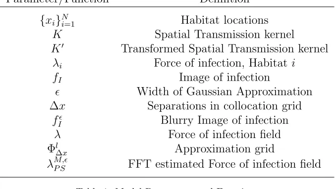
Parameter/Function Definition

{xi}Ni=1 Habitat locations K Spatial Transmission kernel

K0 _{Transformed Spatial Transmission kernel}

i Force of infection, Habitat i

fI Image of infection

✏ Width of Gaussian Approximation

x Separations in collocation grid

f✏

I Blurry Image of infection Force of infection field l

x Approximation grid

M,✏

[image:12.612.141.479.45.236.2]

P S FFT estimated Force of infection field

Table 1: Model Parameters and Functions

in the following section we consider how this assumption can be relaxed.

Two ideas underpin accelerating the calculation of the force of infection (Figure 1). Firstly, the

image of the infectious sources is ‘blurred’ by approximating each delta distribution as a Gaussian

shaped function of width ✏ > 0; this is so that infection potential can be approximated as

origi-nating from grid points. For real populations where individuals are not tied to a point location,

this Gaussian blurring may actually more closely reflect reality. Secondly, we solve an analogous

equation to (6) defined on a discrete collocation grid using efficient FFT convolution solving and

read o↵ { i(t)}N

i=1 directly from a local interpolation scheme.

To this end we introduce a 2-dimensional regular grid over an l _⇥l area, with a spacing x

between grids,

l

x ={i = x(i1, i2) |(i1, i2)2Z2, i2Il}. (7)

These grid-points are the collocation points used for the discrete transformation, that is the points

at which the force of infection is calculated. By varying the spacing x we can use M collocation

points to cover our space, however we always choose x such that l/ x = m 2 N, leading to

(13)

Since our goal is to utilise the efficiency of FFT algorithms we require that both the transmission

kernel and image of infection can be well approximated by their support on the collocation grid. This

will not be true for the delta distributions in the definition of fI since they are not functions in the

traditional sense, but rather distributions in a more general sense [32]. We resolve this problem by

introducing the blurred image of infection, f✏

I, where the delta distributions in the image definition

(5) are replaced by tight Gaussians of width ✏ (>0),

f_I✏(x, t) = N

X

i=1

✏(x xi)Ii(t), ✏(x) = 1 2⇡✏2e

|x|2

2✏2 . (8)

To provide even greater computational efficiency, we treat these Gaussians as having finite range,

cutting o↵at a distance of 5✏. The number of collocation points local to habitati(that are involved

with the blurring of the image of i) is denoted ni =|{i2 l x s.t. |i xi|<5✏}|.

The natural grid-based approximation to the integral form of the force of infection field (6) on

the periodic domainIlis to use a sum over grid points, respecting the periodic boundary conditions,

(i, t)⇡( x)2 X

j2 l x

K({i j}l)fI✏(j, t), (9)

where_{i j_}l represents periodic summation of all distances betweeniand j on a periodic domain,

although in our examples only the shortest vector between points i and j on the periodic space Il

will contribute. The approximation (9) is in the form of a circular convolution sum which can be

efficiently solved (see supporting information) using Fourier (FFT) coefficients of the transmission

kernel ( ˜K) and the blurry image of infection ( ˜f✏

I) and the inverse fast Fourier transform (IFFT)

operation F 1_[_·_],

(i, t) _⇡ M,✏_{P S}(i, t) = ( x)2F 1[ ˜Kf˜_I✏](i, t), (10)

where M,✏_{P S} is equivalently the exact solution to the sum (9) and the discrete Fourier transform, or

(14)

computa-tional burden for its solution everywhere on the grid grows as O(MlnM). Once, we have estimated

the force of infection on the grid of points, l

x, we can read o↵ an approximation for i(t) from

local bilinear interpolation from the 4 grid points nearest xi.

The relationship between the Fourier pseudo-spectra of the ‘true and ‘blurry’ images of infection

is approximately

˜

f_I✏(!, t)⇡˜✏f˜I(!, t), !2Z2, (11)

where ✏ is the zero centred Gaussian (8) and! is a discrete wavenumber for the pseudo-spectrum.

Equation (11) motivates defining a transformed kernel spectrum K˜0_,

˜

K0(!) = K_˜˜(!)

✏(!), ! 2Z

2_. ₍₁₂₎

The approach being to as far as possible reduce the error due to using Gaussian approximations

of delta functions whilst retaining their numerical convenience. Numerical investigation suggests

that using the transformed kernel spectrum (12) improves the accuracy of the pseudo-spectral

ap-proximation to the force of infection field compared to using the discrete spectrum ˜K directly (see

supporting information). A secondary benefit of using the transformed kernel spectrum is to largely

eliminate✏dependence from parameterisation of the FSR simulation scheme. Throughout we choose

✏ sufficiently great so that the mass of the Gaussians (8) is fully supported on the grid (˜✏(0) _⇡1)

but no greater. A detailed error analysis reveals that, without kernel spectrum transformation,

the accuracy of the FSR method depends more strongly upon ✏ with both extremes ✏ _⌧ x and

✏ x being poor parameter value ranges. We refer the reader to the supporting information.

We call simulation using recalculation of M,✏_{P S} and local interpolation the fast spectral rate

re-calculation (FSR) method, and can be represented by the following algorithm.

(15)

1. Choose a suitable FFT algorithm and number of simulation repetitions.

2. Perform one-o↵ pre-calculations:

(a) Calculate and store local points for each habitat i, _{i₂ l

x s.t. |i xi|<5✏}.

(b) Calculate pseudo-spectra of transmission kernel ˜K, zero-centred Gaussian ˜✏ and

trans-formed kernel ˜K0, avoiding zero division error in (12).

3. Choose initial epidemic state, construct the initial blurry image of infection f_I✏(i,0), and set

t = 0.

4. Solve the sum M,✏_{P S}(i, t), ₈i ₂ l

x, by using an FFT algorithm to construct the product

function ˜Kf˜I and taking IFFT using transformed kernel, F 1[ ˜K0f˜I].

5. Re-normalise M,✏_{P S} by the factor ( x)2_{, if this is not performed by the FFT algorithm.}

6. Perform stochastic time-step update using rates of infection i(t) read o↵ from bi-linear

in-terpolation of M,✏_{P S}(i, t).

7. For each ofE events that occurred in step 6., update f✏

I on l x at the ni local points to the

habitat where the event has occurred.

8. If there are remaining infected habitats sett _!t+ 1 and return to 4. If epidemic has finished,

stop simulation.

9. If further simulations are required return to 3. The information calculated in 2. can be reused.

Conveniently, there are a multiplicity of high quality FFT algorithms publicly accessible, for

ex-ample the FFTw library for C programming or the high quality FFT routine in MATLAB. Hence,

there is no necessity for the reader to construct their own transformation algorithm. The

conver-gence and error analysis of random epidemics generated using FSR method onto the ‘true’ random

epidemic defined by dynamics such as (3) is discussed in supporting information.

Although we have chosen to illustrate the use of the FSR method with the motivating example

of the spatial SIR-type epidemic, it should be noted that this methodology holds for any type

of stochastic spatial process where the stochastic rate for events can be written in the form (6).

Examples therefore include a range of spatial epidemiological models (eg SEIR-type and SIS-type

dynamics) and spatial ecological models where a local interaction process governs competition or

(16)

• (Euclidean) Spatially distributed individuals or densities,

• Smooth and translation invariant spatial interactions.

2.3.1. Non-periodic Boundary Conditions

In many real-world applications the idealised periodic boundary conditions are unrealistic:

phys-ical boundaries to transmission may play an important role in containing epidemic spread, or the

habitats may exist in a finite domain isolated from external infection. However, FSR implicitly

requires periodic boundary conditions in solving the convolution sum (10); essentially modelling

the dynamics on a torus rather than a finite plane. To circumvent this problem and yet retain the

efficiency of using FFT we embed our original space, Il, within a larger extended space, Il0, setting

l0 _{> l}_su_ffi_{ciently large such that}_l0 _{periodic extensions of} _{do not interact. This is done by placing}

the habitats in the smaller space Il, and then subsequently creating an empty padded space for f✏ I

on Il0. On this larger space an infection event has a zero probability of ‘wrapping’ round the space

Il0. We achieve this either by restricting to transmission kernels of compact support, or by imposing

compact support by finite range truncation. We therefore set the epidemic on Il0 and use the FSR

method for fast calculation of (i, t) on i₂ l0

x as above.

3. Results

We present results and analyse the accelerated performance due to using the FSR method for

a spatially distributed population of varying size undergoing an SIR-type epidemic. The deviation

between epidemic simulation using direct rate recalculation and simulation using the FSR method

was firstly investigated by comparing their resultant epidemic curves and spatio-temporal

distri-bution of infected habitats at epidemic peak. More systematically error between direct and FSR

simulation was measured using latent variable matching in the sense of Cook et al [31]; essentially

the latent random variables encode the intrinsic stochastic fluctuations of the spatial epidemic

pro-cess and therefore deviation between epidemics with identical latent variables is due solely to error

in the rate calculation. By choosing sufficiently fine grid spacing (small x) it was found that

FSR simulation could be highly accurate even whilst delivering significant time saving per

(17)

to direct simulation as the population size N became larger. We also demonstrate the possibility

of using FSR rate calculation to accelerate likelihood-based parameter inference for this class of

spatial epidemic model. Finally, we present a FSR-simulation case study of continental-scale

epi-demic outbreak amongst commercial US cattle farms, using spatial data that accurately reflect US

agricultural census data at the county scale. E↵ects of farm size on the epidemic dynamics are

introduced without compromising the numerical efficiency of the FSR method.

3.1. Epidemic Spread amongst a Spatial Metapopulation

For the examples in this section the habitat locations are given within a l_⇥l square in two

dimensional space (_{xi}Ni=1 2 [ l/2, l/2]2 = Il ⇢ R2). For simplicity we consider a discrete time

spatial epidemic model conforming to the classic SIR paradigm, such that infected individuals

recover and are then immune. Discrete time steps are chosen to reflect a daily change in disease

status with all rates given in units of (days) 1_{, and therefore the time scale} _t⇤ _{= 1 day. In}

addition to the stochastic infection dynamics (3) there are the additional recovery dynamics; for

each infectious habitat (individual) i the daily probability of removal/recovery is,

P(Rec. event at hab. i | Ii(t) = 1) = 1 exp( ). (13)

Where the recovery rate = 0.1 (days) 1 _{is used in this section; this gives an average infectious}

duration of 10.5 days given the discrete nature of the time-steps. The habitat location coordinates

were chosen as independent spatial Poisson points on Il. The length scales are fixed by choosing

units such that the habitat density N/l2 _{= 1. The length scale of transmission,} _L_{, is given in}

these units. For each N considered, the random distribution of habitat locations was realised once,

with further simulations performed on identical landscapes. Non-periodic boundary conditions as

described above were imposed to replicate the fixed spatial scale of the population.

The transmission kernelK(x, y) encodes the rate of potentially infectious contact from an

infec-tious source at some pointx to pointy. However, in this work we only consider radially symmetric

kernels; that isK(x, y) = K(x0_{, y}0_{) whenever} _|_x _y_|₌_|_x0 _y0_|_{. This is most naturally expressed in}

(18)

range r; in two spatial dimensions the total potentially infectious contact rate in the infinitesimal

range interval [r,r+dr) is 2⇡rK(r)dr. Treating the radially symmetric transmission kernel as an

(unnormalised) spatial density gives three natural summary statistics, independent of the

distribu-tion of susceptibles: the magnitude of the kernel, the mean range of dispersal and the variance in

the range of dispersal.

Magnitude(K) = 2⇡

Z 1

0

rK(r)dr, (14)

Mean(K) =

R1

0 r

2_K₍_r₎_dr

R1

0 rK(r)dr

, (15)

Var(K) =

R1

0 r

3_K₍_r₎_dr

R1

0 rK(r)dr

Mean(K)2. (16)

In the idealised scenario of a uniformly distributed population of susceptibles the summary statistics

define the actual rate of infection and range statistics of successful infections.

The transmission kernel for this section was chosen from the family of Gaussian shaped functions

with width L, _{K(_·;L)_}L>0 such that

K(|x|;L) =

2⇡L2e

|x|2_/₂_L2

. (17)

For l L, sets the magnitude of the transmission kernel over Il independently of length scale

L. The mean and variance of dispersal for the Gaussian kernel in two dimensions are mean(K) =

p

⇡/2Land Var(K) = (2 ⇡/2)L2_{. This directly links the length scale parameter}_L_{to the expected}

range of dispersal of infected habitats. As a reference, in the limit L! 1spatial position becomes

irrelevant and the epidemics collapses into the well understood non-spatial or mean-field stochastic

SIR model with population size N [1, 33] albeit in discrete time. We choose = 0.2 (days) 1_,

where the pathogen can successfully invade except at small values of L.

3.1.1. Performance of FSR method compared to direct simulation

We took as default parameters a metapopulation of N = 12,100 habitats in a 110⇥110 box,

(19)

localised transmission kernel (relative to the scale of the system and the density of habitats) places

a severe test on the FSR methodology. The FSR method was implemented using a collocation grid

of size M = 2562, which gave a grid separation x = 0.5 on an augmented box of side length

110 + 6L used in order to implement non-periodic boundary conditions. Habitat point locations

were approximated as Gaussians of width ✏= 0.4. To initiate the epidemic, a single infected source

farm was positioned in the centre of the box and the 9 closest habitats where also infected.

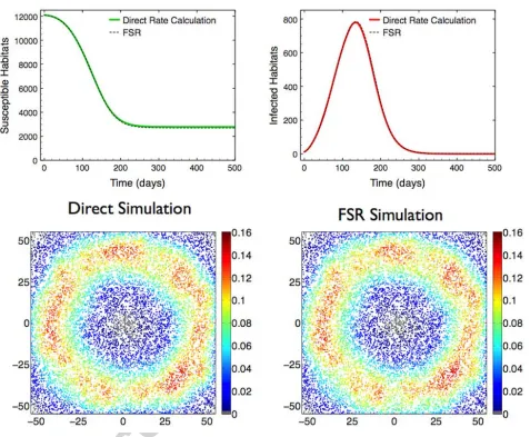
Simulation, using direct rate calculation with 1000 replicates, indicated that epidemic

realisa-tions typically recruit locally to the origin before an invasion front formed, infection then spreading

in a wave-like manner throughout the space causing a declining epidemic tail due to exhaustion

of available susceptible habitats. FSR simulation captured this phenomenology and closely

repli-cated the expected dynamics observed with direct simulation, including the expected peak day

(tpeak= 134 days). The maximum absolute deviation in expected number of infecteds between the

methods, sup_t ₀_{|_hE[(IF SR Idir)(t)]i|} = 16.85 habitats, was small compared to the size of the

metapopulation (0.14% of total metapopulation). Since, in principle, rather di↵erent local spatial

epidemic processes can give rise to similar population level dynamics we also directly compared the

spatial distribution of disease prevalence on the expected epidemic peak day tpeak between direct

simulation and kernel corrected FSR simulation. The probability of each habitat i being infectious

on day tpeak,pi, was estimated using 1000 simulation replicates, and the values compared using

di-rect and FSR simulation; the mean deviation, averaged over all habitats, between the two methods

is small at just 8.5_⇥10 3 _{(Figure 1).}

In order to more efficiently assess the accuracy of the FSR simulation method under variation in

parametrisation we also introduce an alternative error measure based upon the maximum di↵erence

between states in simulations using the direct and FSR methods, but using identical latent variables

Z to account for stochastic fluctuations.

Error =EZ[Error(Z)] =EZ

h

sup t 0

n ₁

N

X

i=1

(20)

where Xdir

i (t|Z) returns the disease state of the ith habitat on day t using direct simulation

condi-tional on latent variablesZ,XF SR

i (t|Z) is the same but where FSR simulation is used, andd(x, y) is

the discrete metric returning 0 i↵x=yand 1 otherwise. This error therefore measures the maximal

di↵erence between the spatial epidemic patterns predicted by the two methods over the entire

epi-demic process. This error measure has the useful property that if FSR returns identical estimates for

{ i(t), t = 0,1, . . . , T_}N

i=1 to direct calculation then Error(Z) = 0, 8Z. Such a relationship would

not hold without matching latent variablesZ, due to inherent variability between epidemic samples.

We conducted a systematic investigation of the error due to using FSR, measured using (18) and

the default parameters above as a baseline comparison; averages were taken over 100 realisations

of the latent variables Z. To initiate the epidemic, a single source farm was placed at the centre

of the space and then surrounding farms where infected such that the initial density of infecteds

I/N = 0.02; this allows us to match initial densities across a range of population sizes N. For the

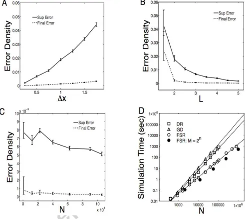
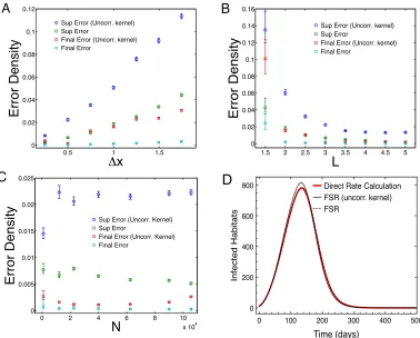
default parameters (N = 12,100, L= 3, x= 0.5), Error = 6.7_⇥10 3 _([6_.₂_⇥₁₀ 3_,₇_.₃_⇥₁₀ 3_{] 95%}

confidence region). The error decayed from baseline at finer grid separation, x (Figure 2A).

Sim-ilarly, error sharply decreased with increasing length scale of infection, L (Figure 2B). Fixing both

transmission length scale (L) and grid width ( x), and taking a sequence of epidemic models with

increasing N (but keeping a constant density of habitats) we found that average error depended

only weakly with N over two orders of magnitude (Figure 2C). These results are in line with both

the intuition that more disperse transmission resolved on at a finer grid scale should lead to better

performance, and the detailed error analysis presented in supporting information.

In addition to supremum (maximum) error over the entire epidemic, it is also of interest to

assess the final error of number and spatial distribution of recovered habitats at the end of the

epidemic. Again matching Z we found the final state error matched the trends observed in the

supremum error, but was generally significantly lower in every part of parameter space (Figure 2).

For our default scenario, the final error density was 3.84_⇥10 4 _([3_.₀₀_⇥₁₀ 4_,₅_.₈₄_⇥₁₀ 4_{]). The}

lower value for final error density suggests that (i) small errors in force of infection calculation due

(21)

the supremum error and (ii) that the large majority of errors are timing errors; that is errors in

when an event occurs rather than whether an event occurs. Dynamically, the latent variables Z

act as a set of thresholds defining when a given habitat has observed sufficient force of infection to

become infected. Therefore, even small errors in the force of infection calculated using FSR have

the potential to change the time-step upon which a habitat becomes infected compared to directly

calculated simulation but are less likely to change whether a habitat becomes infected on any

time-step. No significant systematic bias in the timing of infection was observed in the comparison of

average epidemic prevalence curves generated using FSR and direct calculation, their shapes are

closely similar and agree on expected peak tpeak (Figure 1).

The algorithmic efficiency of the FSR was measured by the time taken to simulate (serially) a

number of replicate complete epidemic realisations; results are presented as an average simulation

time per replicate epidemic (Figure 2D). The initial number of infected habitats was fixed to be the

2% of the total metapopulation size with the default parameterisation outlined above. For most

data points 100 replicate simulations were performed for speed estimates, however, for some of the

large simulations this number was reduced, but never decreased below 20. For large N there was

not great variation in simulation time between individual epidemics. For FSR simulation the main

determinant of speed per time step is the size of the collocation grid M, in order to compare the

speed of FSR simulation to direct simulation we fixed x= 0.5 and N/l2 _{= 1. As a comparison we}

also produced speed estimates for both discrete time simulation using direct rate calculation and

for continuous time simulation based on equation (2) using the popular Gillespie algorithm [34].

For each form of simulation we found a time scaling O(N↵_{) which reflects both the computational}

cost of force of infection recalculation and the number of time steps. Simulation time scaling was

found to be approximately O(N2_{) for both discrete time simulation using direct rate calculation}

(↵ = 1.997) and for continuous time simulation (↵= 2.121). Simulation using FSR delivered

sub-stantial speed benefit (↵= 1.503), which can be further optimised by restricting M = 2n _for_n ₂_N

(↵ = 1.390) (Figure 2D). All simulations used for speed comparison were performed on the same

(22)

The maximum population size we considered for both FSR and direct simulation was N =

105,625 habitats, which is incidentally the same order of magnitude as the number of farms in

Great Britain [35]. At this large population size the FSR method considerably outperformed the

direct rate recalculation in terms of computational efficiency, running simulations in approximately

6.6% of the time. Unsurprisingly, the continuous time simulation algorithm was considerably slower

than either of the other two methods. It is therefore clear that for large scale simulation of spatial

epidemic outbreak together with wide sweeps of parameters space and large numbers of replicates

necessary, the standard GD based simulation is only feasible when dedicated high performance

computing resources are available. However, the use of discrete-time FSR simulation brings this

type of calculation within the realm of powerful desktop computers.

3.1.2. FSR acceleration compared to accelerating direct simulation using pair pre-calculation

We found that for more disperse transmission kernels (larger L) the collocation grid can be

coarsened ( x can be increased) without substantially impairing accuracy and time saving is then

even more dramatic. On the other hand very localised transmission demands very fine grid mesh

for good accuracy, which reduces the time saving due to using FSR. So far we have compared FSR

to the baseline performance of directly simulating the spatial epidemic. We now compare FSR

performance against an alternative acceleration strategy based on exploiting localised transmission.

A simple acceleration technique for simulating the local spread of disease from habitat to nearby

habitat is to pre-calculate e↵ective pairs of habitats; that is those pairs of habitats where an event

at one has a non-negligible e↵ect upon the force of infection of the other. During simulation

epi-demic events at a habitat only cause rate updating at that habitat’s e↵ective pairs which gives an

efficiency saving compared to rate updating at all remaining susceptible habitats, particularly if

each habitat has only a comparatively small number of e↵ective pairs due to localised transmission.

For the Gaussian shaped kernel (17) transmission is unlikely to occur at a range greater than 5L

and we used this range to pre-calculate e↵ective pairs of habitats in a series of simulation speed

(23)

scale L (2  L  17.5) for an entire epidemic. As before habitats were uniformly randomly

dis-tributed across the box Il at unit density (l = 325, N = 105,625) with the 2% of habitats closest

to the centre of Il chosen as the initial infectious set and other parameters as before. The size of

the full set of pre-calculated habitat pairs was therefore _O(N L2_{). FSR simulation used a grid size}

M = 2m _with _m _{chosen as small as possible such that} _{L/ x >} _{6, a ratio of transmission range}

to mesh size above which FSR was found to be accurate. For larger values of L a coarser grid of

fewer points could be used for FSR simulation despite a larger zero-padding domain being required

to avoid periodic boundary transmission.

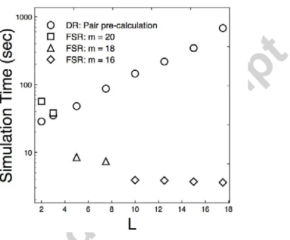
For the most local transmission scale considered (L = 2) direct simulation with pre-calculated

pairs did outperform FSR (direct simulation averaged 28.50 secs per full epidemic simulation, FSR

56.45 secs per full epidemic). The computation time for pre-calculating pairs was not included in

these averages. However, on the desktop used epidemic simulation time increased rapidly withLfor

the pair pre-calculation method despite epidemics with small L typically requiring more time steps

to simulate until the end. By contrast FSR simulation became faster for increasing L reflecting

a typically shorter epidemic and sharply faster whenever a coarser grid could be used (Figure 3).

The cross-over point was at L⇡3, byL= 5 FSR was significantly more efficient at simulating full

epidemics compared to direct simulation with pre-calculated pairs (direct simulation averaged 48

secs per full epidemic simulation, FSR 8.5 secs per full epidemic).

Certainly there exists the potential to further optimise direct simulation through more efficient

pair searching and using systems with greater available RAM. There also exist other methods of

accelerating direct simulation such as the subdivision of Il into cells and exploiting the property

that transmission to distant cells is highly unlikely, an example of such a method is given by

Keeling and Rohani [33]. However, pair pre-calculation is representative of acceleration techniques

for spatial epidemics extant in the literature in that performance improves as transmission becomes

more local. In general these acceleration methods are less successful whenever each habitat has

a large number of e↵ective pairs, whether this is due to long range transmission, heavy-tailed

(24)

for longer range transmission irrespective of metapopulation density, and therefore is a successful

strategy in a di↵erent problem domain from typical acceleration techniques. Heuristically, for very

localised transmission, the force of infection for a susceptible habitat can be compactly represented

as a truncated sum over only a comparatively small number of nearby infectious habitats but

would require many discrete modes for description in the spatial frequency domain used for FSR

convolution solving. The converse is that for disperse transmission a significant fraction of the total

population of infectious habitats contribute to the infection hazard for each susceptible habitat,

whereas in the frequency domain only a comparatively small number of modes are required for a

good description of the force of infection field.

3.2. Accelerated Likelihood Calculation

Likelihood based inference plays an important role in parameter estimation, and hence is key to

matching models with observations. From a classical statistics point of view the maximum likelihood

estimator (MLE), that is the parameter values which maximise the likelihood of the observations,

is viewed as the set of parameters that best captures the dynamics (see Casella and Berger [36] for

an introduction to classical likelihood methods). Additionally, for parameter inference by Markov

Chain Monte Carlo (MCMC) [37, 38, 39] the calculation of likelihood ratios is a necessary, and

often computationally intensive step. Hence the improvement in speed o↵ered by the FSR method

has clear advantages in parameter inference if the results are sufficiently accurate.

As an example of the computational efficiency gains for data imputation derived from using

the FSR algorithm we present a simulated outbreak amongst 19,600 habitats generated using the

simplified model given above. The random habitat locations are given within Il with l = 140 as

the points of a Poisson cluster process [40] chosen so as to give positive spatial correlation between

locations. The transmission kernel was chosen as heavy-tailed,

K(_|x_|) =

(2⇡(1 +|x|2₎₎3/2, K ⇠|x|

3_. ₍₁₉₎

Magnitude(K) = represents the infectiousness of the disease. The target for imputation is the

(25)

removal rate (chosen so that average period of infectiousness was 4 days) and the shape of the

transmission kernel as known data. In keeping with our final example on livestock epidemics, the

parameters chosen here roughly correspond to those for the 2001 UK Foot-and-Mouth outbreak [18].

For a given epidemic realisation we denote the set of populations that are first infected on day

t,_I(t), and the set of populations that are susceptible at the beginning of day tand avoid infection

on that day, S(t). The likelihood L of the observed sequence of infections for a given transmission

rate is given in terms of the per day transmission probabilities [41],

L( |{I(t),S(t)}T

t=0) =P({I(t),S(t)}Tt=0| ) =

T

Y

t=0

h Y

i2I(t)

⇣

1 e i(t)⌘ Y

j2S(t)

e j(t)i_. ₍₂₀₎

The likelihood of a full data set _D, including removals and any other stochastic events, can then

be derived similarly by augmenting with their per day probabilities. We note that calculating the

likelihood (20) involves the sequential recalculation of the daily rates of infection i(t) for each

susceptible population i. This is exactly the task the FSR algorithm has been designed to achieve

with great numerical efficiency.

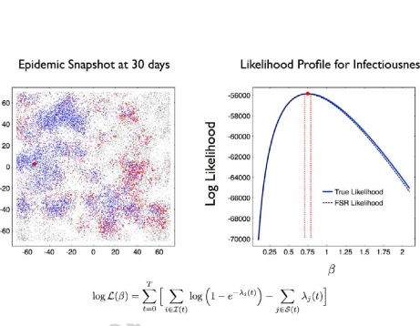
For a randomly chosen initially infected habitat (individual) with infectious intensity true = 0.75

a sample of an invasive epidemic was generated (Figure 4). This outbreak was characterised by long

range invasion of clusters of higher local density of habitats followed by intense spreading within

the cluster. The available data was assumed to be the set of infection and recovery events for the

first 30 time-steps (days) of the outbreak. The log-likelihood profile logLprof ile( ) for the interval

2[0.1,2.1] at a resolution of = 0.01 was calculated from (20) using both direct recalculation

and kernel corrected FSR for the daily infection rates (the approximating grid width used for FSR

was x= 0.5). The constructed log likelihood values were numerically close especially around the

peak, such that not only were the two implied maximum likelihood estimators indistinguishable

ˆ_dir _{= ˆF SR} ₌ _true _{= 0}_._{75, but also the 99}_._{9% confidence intervals} ₂ _[0_.₇₁_,₀_._{79] were also in}

(26)

Constructing the full log likelihood profile using the FSR rate calculation took 16.5% of the time

required to construct the log likelihood profile using direct rate calculation. Such a time saving was

consistent with the accelerated simulation performance found in the previous section (Figure 2D).

The imputation method used in this section was accelerated by using FSR rate recalculation only

because each likelihood calculation (20) was accelerated. This suggests that any statistical method

for the class of spatial epidemic models considered in this work which require repeated likelihood,

or likelihood ratio, calculations could be accelerated by using FSR.

3.3. Case Study: Forecasting Epidemic Outbreak Amongst US Cattle Farms

In this final section we apply the FSR methodology to determine the impact of an epidemic

spreading amongst US cattle farms and to investigate how this depends upon transmission

assump-tions, such as the decay tail of the transmission kernel and the infectious intensity of the disease.

We performed repeated simulations to determine the distribution of epidemic severity using a

mod-ified version of the spatial force of infection (1) that takes into account the numbers of cattle at

both infectious and at-risk susceptible farms. Data for US farm locations and their cattle holding

sizes is only available aggregated at the county-scale. We circumvented this missing information by

generating a synthetic data set of randomised farm locations (with each county) and their cattle

numbers which is consistent with aggregate US agricultural census data at the county level. It is this

synthetic data set of 93,777,559 cattle distributed across 1,018,877 farms that we used to generate

epidemic realisations. The continent-wide nature of the epidemic and the necessity of performing

multiple simulations per parameter choice represented a major computational challenge. The FSR

simulation method presented in this work accelerated simulation sufficiently as to make predictive

Monte Carlo modelling for a range of parameter choices feasible using a standard desktop

com-puter; without an accelerated simulation method this investigation would be impracticable without

far greater computational resource.

3.3.1. Farm Infection Model and FSR Simulation with Demography

The livestock disease being modelled was considered to be sufficiently infectious that once

in-troduced into a naive farm it spread rapidly amongst all the livestock present. This motivates the

(27)

disease progression was represented by two stages, as in Keeling et al. [18] for Foot-and-Mouth

Disease (FMD); an initial exposed (E) period of 4 days during which the infected farm does not

actively recruit to the epidemic and a subsequent actively infectious (I) period of 5 days before

detection and removal. We do not include additional veterinarian tracing e↵orts such as

identify-ing dangerous contacts (DC) of detected infectious farms, or any form of additional control based

on geographic proximity to the detected infectious farm (such as contiguous premise (CP) or ring

culling). Therefore, this model reflects a control e↵ort directed only at removing detected infected

premises (IP) which is the simplest and least disruptive of possible control policies.

We follow Tildesley et al. [24, 42] in extending the basic spatial force of infection (1) to include

a non-linear dependency on the number of cattle (Ni) in both susceptible and infectious farms,

i(t) = Nip N

X

j=1

K(xi xj)NjqIj(t). (21)

The power parameters p, q scale, respectively, the dependence of farm susceptibility and

transmis-sibility upon cattle numbers. For the 2001 FMD outbreak the power parameters for cattle numbers

have been found to vary regionally between 0.2 and 0.44 [24]. We chose p = q = 0.2 for all US

regions which corresponds to the minimal amount of demographic dependence within the inferred

range (p=q= 0 recovers the demography-free model (1)). The FSR collocation grid approximated

a projection of the USA onto a plane with additional zero-padding extending 500 km from the

southern most and eastern most tips of contiguous USA. We chose the FSR collocation grid size

so that M was product of powers of 2 and 3 for numerical efficiency. The grid width was 3.6 km

north/south and 4.6 km west/east, which were a finer scale than the length scales of transmissions

considered below. Gaussian approximations were used with ✏ = 4 km. Simulating epidemic

real-isations with the daily risk model (21) required a small modification to the FSR method. When

updating blurry image of infection f✏

I at local points to farm j a factor N q

j is used to increase the

(28)

simulation with demography is,

i(t)⇡Nip M,✏

P S(xi, t). (22)

The pseudo-spectral approximation for point xi being given by bi-linear interpolation from its 4

nearest collocation grid points. All statistics in this section were estimated from 1000 independent

FSR simulations of a complete epidemic.

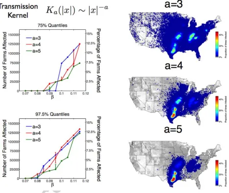
We are interested in the impact on epidemic severity of the decay tail of the transmission

kernel, and moreover how this tail a↵ects the upper quantiles for outbreaks severity, quantities of

considerable public policy importance. To achieve this we simulate outbreaks using a family of

kernels Ka(|x|)⇠|x| a_,

Ka(|x|;L) = Na(L)(L2+|x|2) a/2, a= 3,4,5, (23)

where is the transmissibility of the disease,_N normalises the transmission kernel so that Magnitude(K) =

and L is a length scale parameter. Each transmission kernel is heavy-tailed in the sense of Kot

et al due to each kernel having infinite moments of dispersal distance [20]. Nevertheless, K3 and

K5 represent rather di↵erent transmission tail behaviour within the general family of heavy-tailed

kernels; a consequence of the heavy-tailed decay of K3 is that both mean and variance of the

dis-persal distance (as given by (14) and (16)) are infinite for all L >0 whereas both these dispersal

range measures are finite forK5. Transmission kernelK4 gave an intermediate class of transmission

tail behaviour; Mean(K4) = (⇡/2)L is finite whereas Var(K4) = 1 for L > 0. In the subsequent

simulation study we choose L so that Mean(K5) = Mean(K4) = 20 km. The heavy tailed kernel

K3 cannot be matched in this manner: L= 10 km was chosen as its length scale.

3.3.2. Transmission Tail Decay and Variable Severity

Each epidemic realisation was initiated by a single infectious farm located in Franklin County,

Texas. This choice of initial location can be considered pessimistic from the point of view of disease

(29)

Despite the favourable initial location for the disease the range of epidemic sizes were found to be

multi-modal. For all transmission kernels, and even for the greatest infectious intensity considered

( = 0.115), there was a significant probability of only a small epidemic occurring (Psmall), defined

as at most 50 farms becoming infected. For the finite mean dispersal kernels, with = 0.115, the

probability of a small epidemic probability was similar (Psmall(K4) = 0.428 andPsmall(K5) = 0.434);

whereas for the heavy tailed kernel K3 the probability of a small epidemic occurring was greater

(Psmall(K3) = 0.537).

The most severe epidemic predicted led to almost 140,000 infected cattle farms (13.7% of US

total). For the finite kernels (K4 andK5) those epidemics which do take hold and produce a

nation-wide epidemic were found to be multi-modal in their distribution of final number of disease a↵ected

farms (Figure 5) with both large and intermediate scale epidemics common. The number of farms

a↵ected during a given epidemic realisation reflected that epidemic’s success in invading di↵erent

high-risk regions; in order of most to least likely of having a large-scale outbreak these high-risk

regions are: Texas, the central plains, the Ohio river basin and South-Eastern Pennsylvania (Figure

6). Given this multi-modal behaviour for epidemic sizes it is more natural to focus on quantiles

of outbreak size as a representative statistics for severity. However, epidemics with a heavy tailed

transmission kernel, K3, displayed rather di↵erent behaviour. Epidemic severity with heavy tailed

transmission became strongly bi-modal as the infectious intensity was increased; the epidemics

forecast were either small or tightly clustered around a large epidemic size (Figure 5).

As well as simply examining the number of farms infected, the spatial distribution of these

farms is of important applied interest as it relates to the necessary distribution of control resources.

In all our simulations, the western half of USA largely escaped infection for finite mean kernels.

The infinite dispersal variance kernel K4 had consistently more severe 75% and 97.5% quantiles

of outbreak size compared to K5, and we think of these upper quantiles as reasonable worst-case

scenarios. This reflects that a long-range dispersal event from one farm cluster to a distant one

was more likely for this kernel despite matched mean dispersal range and equal total transmission

(30)

plausible worst-case scenarios for US cattle epidemic forecasting (Figure 6). Risk of infection for

epidemics with heavy tailed transmission kernel K3 was more evenly distributed in space than for

the finite mean kernels K4 and K5. Nonetheless, there are regions in Texas, the central plains, the

Ohio river basin and South-Eastern Pennsylvania where greater risk of infection was observed for

all three kernels, although naturally K3 and K4 shows the greatest spread from the initial source

in Texas.

If we are considering an outbreak of Foot-and-Mouth in the USA, then there is uncertainty in

the transmission constant as well as the shape of the transmission kernel. For a less infectious

dis-ease ( 0.095) the 75% quantiles of outbreak size was significantly smaller for theK3 model than

for the K4 or K5 models. This is because the outbreak is initialised in a region of high cattle and

farm density; therefore more dispersed kernels simply waste infection by placing more transmission

away from this high-density region. Therefore this most dispersed kernel leads to the greatest risk

of early extinction. By contrast for more infectious diseases (0.095 < < 0.115) the 75%

quan-tiles for epidemics with transmission kernel K3 was significantly greater than for the more localised

transmission kernels. The upper extreme 97.5% quantiles for epidemic outcomes with either K3 or

K4 transmission kernel were similar; the ‘worst case’ scenarios for either transmission models were

similar in that either model could predict invasion into a number of important areas for US cattle

farming and further afield. For the most infectious disease intensities considered ( 0.11) the

local transmission kernel K5 also predicted similar 97.5% quantiles (Figure 6).

The predicted spatial patterns of disease incidence and multi-modal severity have important

implications for emergency disease control in response to an epidemic outbreak amongst US cattle

farms. The proportion of outbreaks predicted to cause national-scale epidemics suggests that control

e↵orts based only on removal of IPs, as simulated here, may be insufficient to control disease spread

amongst US cattle farms. This result is in line with findings for the 2001 UK foot-and-mouth

outbreak [18, 43]. The areas at most risk and the overall severity of a predicted outbreak were

found to depend crucially on the tail of the transmission kernel. For transmission kernels K4 and

(31)

and livestock and the ease with which infection can reach an area. This suggests that a regional

(state or county) level control method, such as local movement bans, might be e↵ective at reducing

epidemic burden. In contrast, epidemics predicted using a very heavy tailed transmission (K3),

showed far more limited spatial heterogeneity which combined with the heavier tail suggests that

regionally based control would be unlikely to be successful. This echoes findings for the

heavy-tailed dispersal of sudden oak death in California [44] albeit at a greater spatial scale. Moreover,

the qualitative distinction between predicted epidemic outcomes with K3 kernel and K4/K5 kernels

cannot be explained in analogy to analytic results for simpler models [21, 20, 22] since each kernel

falls into the general ‘heavy-tailed’ phenomenological category. This detailed sensitivity of outcome

upon the tail of the transmission kernel emphasises the need for numerically efficient methods for

forecasting simulations in order to best inform response to epidemic outbreak. The FSR simulation

method is designed to both accelerate the generation of epidemic forecasts and inference techniques

that require repeated calculation of likelihoods.

4. Discussion

We have considered the stochastic simulation of a very common class of models for the spatial

dispersion of an invasive infection. In particular, we have demonstrated a novel method for

recal-culating the stochastic transition rate using a convolution solution that can deliver significant time

saving to large scale Monte Carlo investigations. The convolution solution uses only ‘out-of-the-box’

software for implementation that is readily and freely accessible, moreover the analytic properties

of the error in spectral convolution solving are well understood.

Since the FSR method is an addendum to commonly used stochastic simulation algorithms it is

flexible and is not restricted to solely SIR type spatial epidemic modelling. Rather, the FSR method

is a possible tool for accelerating simulation of models concerned with spatial dispersal where the

dispersion kernel is translation invariant and smooth. It should be noted that the treatment of

habitats as point locations is a simplifying modelling assumption in order to allow the force of

infection to be written as a weighted sum over infected habitats. The FSR method allows the very