Towards Continuous Control for Mobile Robot Navigation: A Reinforcement Learning and SLAM Based Approach

(1)

A reinforcement learning and SLAM based approach

K. (Khaled) Mustafa

MSc assignment

Committee:

dr.ir. T.J.A. de Vries

N. Botteghi, MSc

dr. B. Sirmaçek

dr.ir. M. Abayazid

dr. M. Poel

August 2019

036RaM2019

Robotics and Mechatronics

(2)

(3)

Summary

Mobile robots have attracted intense research interest in recent years due to their numerous potential applications. The capability of autonomous navigation is critical when performing a wide range of tasks including search and rescue missions, ballast tanks maintenance, pipe inspection and activities that are potentially hazardous for humans. Therefore, it is such an exciting and varied topic in the robotics research community.

In literature, various traditional motion planner approaches do exist to solve the autonomous navigation problem for mobile robots. However, most of these approaches assume that a highly precise map of the navigation environment is provided a priori which is not the case, in real life applications, where the exact locations of the obstacles can be hardly obtained. Thus, the motivation for this work is to formulate the mobile robot navigation task in unknown environ-ments as a reinforcement learning problem where (sub)optimal trajectories to desired targets can be realized through trial and error interaction with the environment. Henceforth, a model-free deep deterministic policy gradient approach within an off-policy actor-critic framework is sought that aims at training a motion planner end-to-end to navigate to any random tar-get within the workspace. The motion planner is designed by taking 10-dimensional sparse laser range finder readings, the target position with respect to the robot’s coordinate frame and the previously executed actions as inputs and the continuous linear and angular velocity com-mands as outputs where the robot has to rely on its on-board sensors to perform the navigation task.

The main novelty of this work is to shape the reward function based on the online-acquired knowledge about the environment that the robot gains during training. This knowledge is ob-tained through a grid mapping with Rao-Blackwellized particle filter approach in such a way that the robot can learn a (sub)optimal policy in less number of iteration steps by increasing its awareness about the locations of the surrounding obstacles. To the best of the author’s knowl-edge, this is the first time grid mapping is combined with reinforcement learning to shape the reward function for robot navigation. Additionally, the learned planner can generalize to un-seen virtual environments as well as to a real non-holonomic differential robot platform with-out any fine-tuning to real-world samples.

(4)

(5)

1 Introduction

As the robotics field progresses, robots are being employed in increasingly complicated and de-manding tasks. To accomplish a given task, a robot receives sensory information representing its external environment and takes actions accordingly based on the collected data. The goal for mobile robots is to enhance their behaviour over time by empowering them with high au-tonomous ability based on their incoming experience about the environment. In case a com-plete knowledge about the environment is known a priori, a feasible path to a goal location in the environment can be determined using techniques such as potential field methods [1], graph search [2] and rapidly exploring random trees [3]. Although a lot of progress has been made by those path planning algorithms, they so often require human assistance during set-up time for sensory data acquisition [4]. Additionally, a highly precise map of the environment is required a priori for path planning approaches to work. For this reason, the challenge of au-tonomous navigation in environments with unknown terrain can be formulated as a reinforce-ment learning problem where the agent learns the optimal path through a straightforward trial and error process by interacting with the environment.

In recent years, reinforcement learning has achieved impressive results on a wide variety of challenging tasks like learning to play Atari video games directly from pixels [5] and learning policies for complex continuous control problems that involve locomotion and manipulation [6; 7], etc. In robotics, in particular, deep learning and deep reinforcement learning have sim-ilarly achieved impressive results. Thanks to it, robots are now capable of learning complex manipulation tasks like opening a bottle [8], putting cloths on a hanger [9], and precisely fit-ting small pieces into a larger structures [10]. Because reinforcement learning agents can learn without expert supervision, the type of problems that are best suited to reinforcement learning are complex problems where no obvious or easily programmable solution does appear. Re-inforcement learning enables a robot to autonomously discover an optimal behavior through trial-and-error interactions with its environment. During this interaction, the robot perceives the environment through its sensorsSand affects the environment through a set of actionsA

performed by its actuators. Instead of explicitly detailing the solution to a problem, in rein-forcement learning, the designer of a control task provides feedback in terms of a scalar objec-tive function that measures the one-step performance of the robot. In other words, by applying an actionat ∈A, the agent is able to change its own statest∈Sand the state of the

environ-ment and consequently it receives a rewardrt∈Rfor being in the new state. The reward is the

way of teaching the agent whether the action taken in that state is good or bad. Accordingly, the optimal mapping from states to actions, called optimal policyπ∗(a|s), can be discovered by maximizing a predefined accumulated reward that reflects the quality of the trajectory taken by the robot.

In reinforcement learning context, the reward function is one of the most essential and effec-tive parts since it is the only way by which the agent can evaluate its performance. Hence, a good reward often makes a difference between a tractable learning problem and an intractable one as will be discussed in section 5.2. For this reason, a novel idea to condition the reward signal on the knowledge of the environment is presented in this thesis.

(10)

1.1 Related Work

In literature, lots of proposed learning approaches do exist that enable a robot to learn naviga-tion acnaviga-tions using on-board sensory informanaviga-tion in environments with known and unknown flat terrain. Benefiting from the improvement of high-performance computational hardware, these methods are mainly based on deep reinforcement learning. In [11], a successor feature deep Q-Network (DQN) based reinforcement learning is proposed to solve the navigation prob-lem when a map of the environment is known a priori. The main focus is to transfer the knowl-edge from one environment to another where the input is depth images obtained through a kinetic sensor and the output is discrete actions including standing still, turning 90◦right or left or going straight for 1m. The trained controller was transferred to a new environment on a physical mobile robot, and additional training was conducted. Experiments in the same en-vironment showed that the number of additional training is less than having to train a new network from scratch. In [12], Asynchronous Advantage Actor-Critic (A3C) approach was pro-posed to help a robot moving out of a random maze for which a map is given. The input to the system includes 2D map of the environment, the robot’s heading and the previous estimated pose whereas the output is the navigation actions such as move (forward, backward, left, right) and rotate (left, right) to a given target location. Furthermore, in [13], an external memory act-ing as an internal representation of the environment for the agent is fed as an input to a deep reinforcement learning algorithm. In this way, the agent is guided to make informative plan-ning decisions to effectively explore new environments.

Although the aforementioned literature shows the feasibility of using deep reinforcement learning to learn navigation policies using high dimensional sensory inputs from the environ-ment, they suffer from two main problems. The first one is that their navigation actions are simply discrete like move forward, turn left and turn right which may lead to rough navigation behaviors. Moreover, in all these methods, the map of the environment was provided to the robot a priori where the robot is trained to navigate through this map without human assis-tance. However, there are two issues regarding providing a map a priori for a training method. The first problem is regarding the time-consumption needed for building the obstacle map, whereas the second one is the high dependency of these approaches on the preciseness of the built map. Hence, in this thesis, it is aimed to design a learned motion planner that produces continuous control actions to navigate a mobile robot to a desired target. The contribution of this work is that no map is provided to the robot beforehand. However, instead, the robot builds a probabilistic map of the environment online during training and uses this map to shape its reward function. In this way, the robot gets more awareness about the surrounding obstacles which enables it to figure out a navigation policy in less iteration steps.

1.2 Problem Formulation and Challenges

Although deep reinforcement learning has achieved tremendous results where a key represen-tative of this advancement is the application of reinforcement learning to the Go game [14] that was once considered the most challenging problem in the artificial intelligence community [15], robotics hold several unique challenges for learning algorithms compared to other fields. Accordingly, a naïve application of reinforcement learning techniques in robotics is likely to be doomed to failure. Hence, it is instructive to emphasize on some challenges faced in robotics learning. The following points give more insight regarding the main challenges that can be encountered while applying reinforcement learning algorithms in robotics.

(i) Many tasks of interest in robotics have continuous and high dimensional action spaces which limits the application of deep Q-Networks1to such problems since they rely on finding the action that maximizes the action-value function which would be

(11)

tionally exhaustive in continuous control tasks. A direct solution to this problem is to discretize the action space, however this has many limitations among them is the curse of dimensionality. In 1957, Bellman coined the termCurse of Dimensionalitywhen he faced an exponential explosion of the number of actions with the number of degrees of freedom in discrete high dimensional spaces. For instance, a 7 degree-of-freedom robotic arm with a coarsest discretizationai∈{−k, 0,k} for each joint leads to an action

space with dimensionality: 37=2187. The problem becomes even worse when a finer discretization is required. This exponential growth in the number of states leads to very slow convergence rates of the reinforcement learning algorithm.

Hence, to tackle this problem, in this thesis, it is focused on the navigation problem of non-holonomic mobile robots with continuous control through deep reinforcement learning, which is an essential ability for the most widely used robots. This is achieved by adapting a policy search based learning approach that is discussed in section 3.4.

(ii) Another problem for learning in robotics is that it is often unrealistic to implement the training procedure in the real world. The reason is that the trial-and-error process may lead to a serious damage to real systems. Furthermore, obtaining real data from robotic systems can be extremely difficult and time-consuming. Thus, applying reinforcement learning in robotics demands safe exploration which becomes a key issue of the learning process, a problem often neglected in the general reinforcement learning community, due to the use of simulated environments. Additionally, the dynamics of the robot can change, during learning, due to several external factors including wear and tear of phys-ical components and thereby the learning process may never converge.

Fortunately, simulation with accurate models could potentially be used to offset the cost of real-world interaction. One of the most powerful simulation platforms in robotics community is Gazebo in the sense that it is more realistic with respect to the underlying physics and the sensor noise compared to other simulated environments [16]. In an ideal setting, this approach would allow to learn the behavior in simulation and subsequently transfer it to the real robot.

(iii) The reward function can be considered the most important component within the rein-forcement learning framework since it is the only way by which the agent can evaluate its performance while training. In contrast to traditional reinforcement learning algorithms, it is challenging to define a good reward function for the robot task since sparse reward can barely succeed in robotics applications. Therefore, it is necessary to design a proper reward function that takes into account the features of the space in which the agent robot operates and the available knowledge of the environment. Adjusting the reward function based on the task at hand is called, in literature, reward shaping which is considered as the main contribution of this thesis.

(12)

1.3 Proposed Method

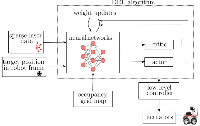
[image:12.595.89.471.380.621.2]

As mentioned beforehand, the main purpose of this research is to design a deep reinforcement learning algorithm that uses raw sensory data from the robot’s on-board sensors to determine a series of primitive navigation actions for the robot to execute in order to traverse to a goal location in an environment with unknown flat terrain. The advantage of deep reinforcement learning is that it can directly use raw sensory data to determine robot navigation actions with-out the need for pre-labeled data. In section 1.2, it was discussed that policy search methods are more suitable for physical control tasks. For that reason, a model-free off-policy1actor-critic al-gorithm based on deep deterministic policy gradient is presented within the framework of this thesis to solve the navigation problem for non-holonomic mobile robots. To achieve this goal, two neural networks are introduced where one of them works as the actor whereas the other is the critic. The aim of the actor network is to determine the optimal deterministic policy that maps the states, which are given as raw laser range findings data and the target’s position in the robot’s frame to navigation actions in the form of continuous linear and angular velocities. Here, it should be pointed out that the deep-RL algorithm represents thehigh-level controllerof the robot. Once the robot’s navigation actions are determined, the robot’s low-level controller executes each action by sending the appropriate commands to the actuators. The critic net-work then evaluates the quality of taking a particular action from a certain state by computing an action-value function. Afterwards, the parameters of the actor network are then adjusted in the direction of the gradient of the action-value function which is discussed in section 3.4. This process continues iteratively until an optimal policy is realized.

Figure 1.1:Proposed architecture for continuous control navigation in unknown environment. The motion planner is trained through a deep-RL within an off-policy actor-critic framework that represents the high level controller of the robot using only sparse laser data. The robot’s low level controller executes the navigation actions determined by the motion planner. The occupancy grid map

is built online by the robot and used to shape the reward function.

As a matter of fact, since the reward function has a direct impact on the learning rate of the re-inforcement learning algorithm, the available knowledge of the environment is incorporated

(13)

in the reward function. This knowledge is represented by the online-acquired occupancy-grid map that the robot gets while learning through adopting a occupancy-grid-mapping with Rao-Blackwellized particle filters. This SLAM technique is used due to its computational efficiency which is a key factor in deep reinforcement learning algorithms along with the fact that it can be simply integrated in robot operating system ”ROS”; the main middleware framework on which the proposed algorithm is implemented. A comparison is then made to evaluate the dif-ference in performance between the standard reinforcement learning technique and the one combined with SLAM. Here, it should be pointed out that SLAM is not the main concern of this research, however instead, it is just used as a tool to improve the learning algorithm. The architecture of the proposed framework is depicted in Figure 1.1 where the main modules are discussed in detail throughout this thesis.

Moreover, a major challenge of learning in continuous action space is exploration especially since the algorithm adopted learns a deterministic policy. However, an advantage of the off-policy algorithm is that the exploration problem can be treated independently from the prob-lem of learning. In other words, it is possible to learn a deterministic policy while following a stochastic behavioral policy for exploration purposes. Therefore, different exploration policies are introduced including action and parameter space policies.

1.4 Research Questions

To fulfill the required tasks discussed in the previous section, the following two main research questions are formulated:

RQ1. How the navigation problem of non-holonomic mobile robots can be formulated as a reinforcement learning problem that could be solved by using deep deterministic policy gradient (DDPG) actor-critic algorithm?

RQ2. To what extent does the incorporation of the partial map obtained about the environment via the SLAM algorithm improve the learning algorithm?

From these main research questions, further sub-questions arise which can be articulated as follows:

RQ3. How to determine a proper reward function that can reflect the quality of the learned trajectory?

RQ4. How applicable is it to generalize the learned policy on one environment to another environment through transfer learning?

RQ5. What is the effect of different exploration noise on the quality of the learned trajectory and the learning rate?

RQ6. Is it possible to transfer the learned policy on the virtual environment directly to the real robot?

The rest of this thesis is dedicated to answer these research questions.

1.5 Report Layout

(14)

(15)

2 The Reinforcement Learning Problem

This chapter provides an overview of the reinforcement learning problem, presenting the mathematical background behind the solution of the decision making problem, and explain-ing the methods upon which this research is built.

In general, machine learning techniques can be typically classified into three broad cate-gories: supervised learning, unsupervised learning and reinforcement learning. These three approaches differ by the type of feedback they receive to learn. In supervised learning, the learning agent is provided with a data-set of labeled examples, each contains a description of a situation as well as the correct classification of this situation or action to take when confronted by it. The objective of the learning is then to extrapolate this training data-set and be able to determine the correct classification or action to take for unseen situations. Unsupervised learning algorithms, in contrast to supervised learning, have no access to output values and therefore try to find hidden parameters and structures within the data by creating clusters that can group the given data. On the other hand, reinforcement learning is different from both previously described categories.

Reinforcement learning is a branch of machine learning that deals with sequential decision making. RL is a problem in which the agent, also called a decision maker, interacts with the environment. In the context of robotics, in this interaction, the agent senses the environment through its on-board sensors and responds to the environment through actions performed by its actuators. Based on these actions, the agent receives a scalar reward which is a way of letting the agent know how good or bad it was to take that action from this particular state. The fun-damental idea of reinforcement learning is to learn anoptimal policy, which is a mapping from states to a probability distribution over actions, that maximizes the expected sum of rewards in an attempt to achieve a desired goal. RL is different from supervised learning in the sense that in RL the agent does not know a priori what the right action is at the particular instant. How-ever, instead, it must figure that out based on a trial and error interaction with the environment [17]. In episodic settings, where the task is restarted after each time the episode is over, the goal of the agent is to maximize the total reward per episode. However, if the task is on-going, there is no clear beginning and end, the aim is either to maximize the average reward of the whole life-time or a weighted average reward where the distant rewards have less influence.

The interaction model between the agent and the environment can be modelled as a Markov Decision Process (MDP) [18] which is described in detail in the next section.

2.1 Markov Decision Process

In the robotics context, the agent can be considered as the high level controller of the robot which is responsible for decision making [19], i.e. the required velocity that should be re-quested from the motors. The aim of reinforcement learning is to control this agent by finding an optimal policy by which the agent’s can determine its optimal actions. The thing that the agent interacts with, comprising everything else outside the agent, is called the environment. This includes even the robot’s sensors and actuators. The agent and the environment interact continually where the agent selects actions and the environment responds to these actions and presents new situation to the agent. This interaction process between the agent and the envi-ronment is modelled as a Markov decision process.

A Markov decision process is a discrete mathematical framework forsequential decision mak-ingwhich consists of five components that can be formally represented by a tuple [18]

M₌¡

(16)

where: S is a finite set of states which contains the information about the environment that is available to the agent at a discrete time-stept; an example would be the current position of a robot in a navigation task. A₌{a1, ...,ak} is a set of actions the agent can perform on the

environment; an example could be the linear and angular velocities of a robot. Not to mention that both the states and actions can be either discrete or continuous sets. The probability of ending up in statest+1when performing an actionat in the statest is restricted to satisfy the

Markov property given by

P(st+1|st,at)=P(st+1|s1,a1, ...,st,at) (2.2)

In other words, the Markov property states that the transition fromst tost+1depends exclu-sively on the previous statest and actionat and not on additional information about the past

states or actions. Moreover, the transition probability captures the dynamics of the environ-ment. R(st,at) is the reward function that gives the agent a feedback from the environment.

This feedback is given in terms of a scalar signalR(st,at)∈Rafter the agent performs an action

atfrom the statestand is assumed to be a function of the state. This gives a rise to a sequence

[image:16.595.121.444.433.672.2]

(s0,a0,r1,s1,a1,r2, ...) that is rolled out by the agent in the environment. As a matter of fact, the reward function specifies the goal of the reinforcement learning problem. The last component of the Markov Decision Process is the discount factorγ∈[0, 1] which is used to determine how much the future rewards should influence the accumulated reward, also called as the return. Ifγis close to 0, the return evaluation will be myopic and may result in poor performance, whereas, it will be ”far-sighted” whenγis close to 1, i.e., the closerγis to 1, the more effect future rewards would have on the return. Here it should be pointed out that in some reference, the discount factorγis considered as a part of the MDP [19; 20; 21] while in other definitions it is regarded as an additional parameter where both conventions are widely used in literature. The Markov Decision Process in the context of robotics is depicted in Figure 2.1:

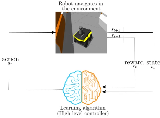
Figure 2.1:The reinforcement learning loop in the context of robotics. At timet, the agent receives a statestfrom the environment. The agent uses its policy to choose an actionat. Once the action is executed, the environment transitions a step, providing the next statest+1as well as feedback in the

form of a rewardrt+1. The agent uses knowledge of state transitions, of the form (st,at,st+1,rt+1) in

(17)

Figure 2.1 can be related to Figure 1.1 in the sense that the brain of the robot, the agent, can be resembled by the DRL algorithm depicted in Figure 1.1 while everything else represents the environment that the agent interacts with.

2.2 Reinforcement Learning Bricks

In this section, the fundamental background for reinforcement learning is discussed that is essential for understanding this thesis.

Definition 2.2.1. LetRtbe the immediate reward at time stept, andγ∈[0, 1] be the discount

factor. The returnGt, is then defined as

Gt= T

X

k=0 γt_R

t+k+1 (2.3)

whereT is the last time step in the interaction between the agent and the environment. The planning horizon can be finite, as the case in episodic tasks [19], or infinite, as in continuing tasks whereT = ∞. γ<1 prevents an infinite sum of rewards from being accumulated. The reward defined in 2.3 represents the reward over a single sample across the environment, and thus, no expectation is required at this stage.

In Markov decision process, the goal is to find a policy, denoted byπ, that maximizes the cu-mulative return. The policy describes the agent’s way of behaving in the environment since it determines the next action the agent should take from any given state. The policy can be either deterministicπ(s) or stochasticπ(a|s). A deterministic policy always returns the exact same ac-tion from a given state in the form ofa=π(s), whereas a stochastic policy models a conditional probability distribution over actions and then draws an action according to this distribution a∼π(a,s)=p(A₌a|S).

Definition 2.2.2. A deterministic policy is a functionπ(s) that maps states into actionsS→A, whereas a stochastic policyπ(a,s) :S_→p(A₌a|S) is a mapping from a state to a probability of taking a specific action.

Another important concept in RL is the state-value functionVπ(s). This function represents the assessment of how good it is for the agent to be in a given state in terms of how much future reward can be accumulated from this state [18]. The state-value function can be calculated by the expected amount of reward the agent can expect to get from stateswhen following policy π.

Definition 2.2.3. The state-value functionVπ(s) of a states, under the policyπcan be defined as:

Vπ(s)=Eπ[Gt|st=s]=Eπ "

∞

X

k=0 γk_R

t+k+1|st=s

#

,∀s∈S (2.4) whereE_π[.] is the expectation operator for policyπthat the agent follows..

The value function of statest can be expressed in terms of the immediate reward and a

dis-counted value of the successor state st+1. This recursive relationship betweenVπ(st) and

Vπ(st+1) is known asBellman’s expectation equation[22] that can be derived starting from the definition of the state-value function given in (2.4).

Vπ(st)=E[Gt|st=s]

=E£

Rt+1+γRt+2+γ2Rt+3+...|st=s¤

=E£

Rt+1+γ¡Rt+2+γRt+3+...¢|st=s¤=E£Rt+1+γGt+1|st=s¤

=E£Rt+1+γVπ(st+1)|st=s

¤

=X

a π

(a|s)

Ã

Rt+1+γ

X

st+1

p(st+1|s,a)Vπ(st+1)

(18)

The reason why an expectation does exist in the state-value function is due to the fact that the underlying policy is stochastic. Thus, it is required to average over all possible actions that can be taken from this state. Furthermore, since the transition from one state to another after tak-ing a certain action is not deterministic as it is conditioned by the transition model imposed by the dynamics of the environment, it is also obliged to average over the state-value function of all successive states. Here it is worth mentioning that a state might have a high value de-spite having a low immediate reward, because it regularly leads to other states that yield high rewards.

Similarly, it is possible to define the value of taking an actionafrom a statesand following a policyπthereafter. This is called the action-value function or quality function and is denoted asQπ(s,a). The action-value function is closely related to the state-value function but it is also conditioned by the actiona. In other words, instead of measuring the value of being in a par-ticular state, it measures the quality of taking an actionafrom a states. As will be shown later, the advantage of using action-value function over state-value function is that no model of the environment is needed to figure out the optimal policy which makes it suitable for model-free approaches.

Definition 2.2.4. The action-value functionQπ(s,a) for a given state-action pair (s,a) under policyπis defined as:

Qπ(s,a)=Eπ[Gt|st=s,at=a]=Eπ "

∞

X

k=0 γk_R

t+k+1|st=s,at=a

#

(2.5)

whereE_π[.] is the expectation operator for policyπthat the agent follows.

As mentioned previously, the goal of an agent is to learn a policyπ(find a sequence of actions through an MDP) that maximizes the expected return of a stateVπ(s). A policyπis said to be better than or equal to a policyπ0if the expected return it generates is greater than or equal to that ofπ0for all states, such as:

π≥π0⇐⇒Vπ(s)≥Vπ0(s),∀s∈S

For all MDPs, there exists at least one policy that is better than or equal to all other policies. This is called the optimal policyπ∗. Accordingly, the optimal state-value function is the function that corresponds to the optimal policy and can be defined as:

V∗(s)=max

π V

π_(s), _∀_s_∈_S _(2.6)

Similarly, the optimal action-value function is defined as

Q∗(s,a)=max

π Q

π_(s,_a), _∀_s_∈_S_,_∀_a_∈_A _(2.7)

The Bellman equation for the optimal state-value functionV∗(s) results in theBellman opti-mality equation. The interpretation of the Bellman optiopti-mality equation is that the value of a state evaluated for an optimal policy must be equal to the expected return when in statesand picking the best action from this state.

V∗(s)= max

a∈A(s)Qπ∗(s,a)

= max

a∈A(s)Eπ∗

Ã

∞

X

k=0 γk_R

t+k+1|st=s,at=a

!

= max

a∈A(s)

Ã

Rt+1+γ

X

st+1

p(st+1|st,a)V(st+1)

!

(19)

the best action from each state, where best means the action that maximizes the value of the next state in each state. This also applies to the action-value function resulting in Bellman optimality equation forQ∗

Q∗(s,a)=X

st+1

p(st+1|s,a)

µ

Rt+1+γmax

at+1

Q(st+1,at+1)

¶

(2.8)

In case the transition probabilities and the reward functions are known, the Bellman opti-mality equation can be solved in an iterative fashion. This approach is known as Dynamic programming-based optimal control approach such as policy iteration or value iteration. The algorithms which assume these probabilities to be known or estimate them online are collec-tively known asmodel-basedalgorithms. But for most other algorithms, they assume the prob-abilities are not known and they estimate the policy and value functions by performing rollouts on the system. These methods are known asmodel-freealgorithms. Monte Carlo, temporal dif-ference and policy search methods are the most common model-free algorithms used. In most of practical scenarios, an explicit model of the environment is not given a priori and it also requires high computational time to build this model. Thus, in the robotics context, it is pre-ferred to use model-free learning approaches [19]. For this reason, model free algorithms are discussed in the next section. The reader who is interested in model-based algorithms can refer to Appendix A where they are discussed briefly.

2.3 Model-free Methods

Model-free methods can be applied to any reinforcement learning problem since they do not require an explicit model of the environment. Model-free methods can be generally classified into two categories, mainly value function based approaches and policy search methods. In value function based approaches, the agent tries to learn a value function and infer an optimal policy from it. On the other hand, in policy search methods, the agent directly searches in the space of the policy parameters in an attempt to find an optimal policy. There is also a hybrid, actor-criticapproach, which employs both value functions and policy search [19].

Model-free approaches can also be classified as being either on-policy or off-policy. On-policy methods use the same policy for both generating actions and updating the current policy. How-ever, on the other side, off-policy methods use a different exploratory policy to generate actions as compared to the policy which is being updated. The following subsections look at various model-free algorithms used as well as both value function and policy search based methods.

2.3.1 Value function based Methods

2.3.1.1 Monte Carlo Methods

Unlike dynamic programming discussed in Appendix A, Monte Carlo methods do not assume a complete knowledge of the environment’s dynamics. However, instead, they require sample sequences of states, actions, and rewards obtained through interactions with the environment [18]. Monte Carlo methods estimate action-value functionsQπ(s,a) by averaging the returns observed after visiting these states in the previous episodes. Thus, in order to ensure that well-defined returns are available, learning is only possible in episodic tasks. Furthermore, the problem is non-stationary; since the return of a state upon taking an action depends on the sequence of actions taken in post-states and the selection of the actions is undergoing learn-ing. To handle this issue, Monte Carlo methods adopt the same idea of general policy iteration discussed in Appendix A, however, they differ from dynamic programming in the sense that they are based on a sample of experienced sequences rather than on a complete distribution of all possible scenarios. The value functions and corresponding policies interact to obtain an optimal policy:

π0

PE

−−→Qπ0_→₋I π

1

PE

−−→Qπ1_→₋I π

2...

I

−

(20)

Alternating between evaluation and improvement happens on an episode-by-episode basis. The observed returns of an episode are used for policy evaluation, and then the policy is im-proved at all the states visited in the episode. These methods converge to the optimal policy Qπ∗ as the number of visits to each action-state pair approaches infinity. The corresponding greedy policy for any action-value functionQ, is the one that for eachs∈S, chooses an action deterministically with maximal action-value:

π∗_(s)₌_argmax

a∈A

Q(s,a)

There are two main Monte Carlo methods that differ in the way in which the average return is calculated:

1. First Visit MC method: estimates the action-value function as the average of the returns following the first visit to the state-action pair in every episode.

2. Every Visit MC method: estimates the action-value function as the average of the returns after every visit of the state-action pair in every episode.

To summarize, Monte Carlo methods differ from dynamic programming methods in two major ways. Firstly, they can be used for direct learning without a model of the environment. Sec-ondly, they do not bootstrap, which means they do not update their value estimates based on the value estimates of the successive state. Though Monte Carlo methods are straightforward in their implementation, they require a large number of iterations for their convergence and suffer from a large variance in their value function estimation since they use the actual return from every visited state till the end of the episode where this return suffers from noise. For this reason, temporal difference learning is discussed in the next section.

2.3.1.2 Temporal Difference (TD) Learning

Temporal difference methods combine ideas from both dynamic programming and Monte Carlo methods [23]. Like dynamic programming methods, TD methods execute bootstrapping which means that they update their estimates partly based on previous estimates, however, they use samples as Monte Carlo methods. While Monte Carlo methods need to wait until the end of the episode to determine the increment in the value function, one step TD method waits only until the next time step to execute the updates. Accordingly, instead of using the total ac-cumulated reward, TD methods calculate a temporal error, which is the difference between the new and old estimates of the value function, by considering the reward received at the current time step and use it to update the value function. This kind of update reduces the variance but increases the bias in the estimate of the value function since it doesn’t use the actual return in updating the value function estimates. The update equation for the value function is given by:

Q(st,at)=Q(st,at)+α





rt+1+γQ(st+1,at+1)

| {z }

TD-target

−Q(st,at)





 (2.9)

whereα∈[0, 1] is the step-size parameter that determines how much the Q-value is updated, rt+1is the reward received at the current time step,st+1is the new state andst is the old state.

The algorithm keep repeating until the loss function (TD error) reaches a small value. Two TD algorithms which have been widely used to solve reinforcement learning problems are SARSA (acronym for State- Action-Reward-State-Action) and Q-Learning.

(21)

Algorithm 1SARSA

InitializeQ(s,a)∈Rrandomly,∀s∈S,∀a∈A. repeat

Initializes1

Select an actiona1using a policy derived fromQ(s,a), (e.g.²-greedy) for t=1 :T do

Take actionat, observe rewardrt+1and new statest+1.

Choose next actionat+1using policy derived fromQ(s,a), (e.g.²-greedy) UpdateQusing

Q(st,at)←Q(st,at)+α¡rt+1+γQ(st+1,at+1)−Q(st,at)¢

end for untilterminated

It is clear that SARSA is an on-policy algorithm since the behavioral policy for exploring the environment is the same as the update policy. Hence, this method is not preferred in case a deterministic policy is used for updating the Q-values since in this case it is not guaranteed to explore the entire workspace sufficiently. Therefore, in [24], an off-policy temporal difference algorithm known as Q-learning is introduced. In Q-learning, the post-actionat+1is selected by maximizing the Q-value of the next stateQ(st+1,at+1) instead of following the current policy. Thus, Q-learning belongs to the off-policy category. The Q-learning algorithm is summarized below:

Algorithm 2Q-learning

InitializeQ(s,a)∈Rrandomly,∀s∈S,∀a∈A. for allepisodedo

Initializes1

Choose actiona1using policyπ(s) derived fromQ(s,a), (e.g.,²-greedy) repeat

for each stept in an episodedo

Take actionat, observe rewardrt+1and new statest+1. Choose next actionat+1using policyπ(st+1).

UpdateQusing

Q(st,at)←Q(st,at)+α

µ

rt+1+γmax

at+1

Q(st+1,at+1)−Q(st,at)

¶

end for untilterminated end for

(22)

Learning

Monte Carlo Dynamic

Programming

Exhaustive Search Full

Backups

Sample

Backups Bootstrapping

Shallow Deep

Backups Backups

(c) Temporal-Diﬀerence

(a) (b)

[image:22.595.147.413.72.282.2]

(d)

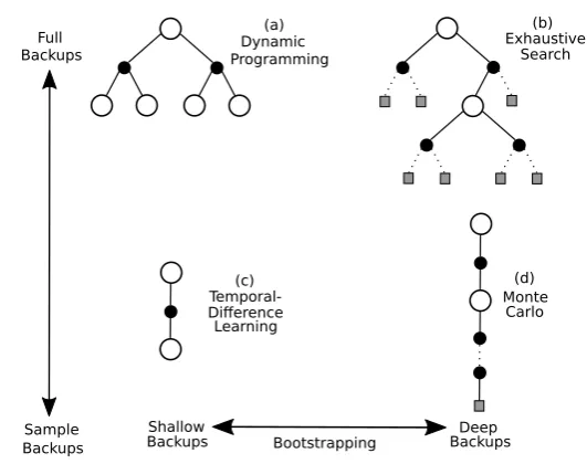
Figure 2.2:Two dimensions of RL algorithms, based on the backups used to learn or construct a policy. At the extremes of these dimensions are (a) dynamic programming, (b) exhaustive search, (c) one-step TD learning and (d) pure Monte Carlo approaches. Bootstrapping extends from (c) 1-step TD learning, with (d) pure Monte Carlo approaches not relying on bootstrapping at all. Another possible dimension of variation is choosing to (c, d) sample actions versus (a, b) taking the expectation over all choices.

Recreated from [18].

action will be executed:

at=







random action, with ²- probability argmax

a

Q(st,at), otherwise (2.10)

This is used to let the agent discover states that might not be visited a lot of times in order to update the Q-value for these states, which could eventually lead to better policies. In most of the cases, it is preferred to start by a large number of²to encourage the robot to explore most of the environment and then decrease this value by a decay rate to exploit the best obtained trajectories. This is known asExploration-Exploitation trade off.

As a recap for value-function based approaches, Figure 2.2 depicts the main differences be-tween dynamic programming, Monte Carlo methods and temporal difference learning.

2.3.1.3 Function Approximators

Function approximation is a family of mathematical and statistical techniques used to rep-resent a function of interest when it is computationally intractable to reprep-resent the function exactly or explicitly. The easiest way to save the values of a value function for different states is in a tabular form. However, if the state space of the problem is large, it becomes impossible to store all the values in a tabular format. The reason is not only due to the fact that storing this data would require extremely huge amount of memory but also looking up some value for a particular state will require an entire sweep of the table which is computationally expensive. In addition, if the state space is continuous, a tabular format will become impossible. Here it is worth mentioning that the problem is not limited only to the large amount of memory required to store the table, but also to the large number of data and time required to estimate each state-action pair accurately. In other words, it is required to generalize the experience gained on a subset of state-action pairs to approximate a broader set.

To overcome this problem, function approximators are used to store a value function. Instead of a table, the value function can be parameterzied by a vectorθ=[θ1,θ2, ...,θn]T that

(23)

approxima-tor can be thought of as a mapping from a vecapproxima-torθ inRn to the space of the value function. Nowadays, artificial neural networks (ANN) are widely used as function approximators. The advantage of using neural networks is due to their capability to represent complex value func-tions with lesser number of parameters. This reduces training time for reinforcement learning algorithms for high dimensional systems and is less memory extensive. However, despite the advantages of neural networks as function approximatros, applying them directly to reinforce-ment learning problem results in unstable performance. Thus, additional modifications are required to enable them to be applied effectively as discussed in section 3.2. Before describing the techniques in deep reinforcement learning, some theory of deep learning is needed which is introduced in section 3.1.

2.3.2 Policy Search Methods

In previous sections, it was shown that it is possible to derive reasonable performing policies from good estimates of value functions. However, because policies derived from value func-tions search over a discrete number of Q-values, it is not possible to directly obtain policies that output continuous actions using one of these methods described before. For this reason, policy search methods are analyzed in this section.

Policy search methods are another class of reinforcement learning algorithms that use param-eterized policies π_θπ that can be completely described by the parameter θπ and thus

pro-vide maximal freedom to learn any action-generating function. To evaluate different poli-cies, the expected return followingπover all trajectories conditioned by the policy, formally τ∼p_π(τ)=p(τ|θπ), is used wherep(τ|θπ) is the probability distribution over sampled trajecto-ries. The return over a single trajectoryr(τ) is given by

R(τ)=

T−1

X

t=1 γt−1_r

t+1 (2.11)

The termrt+1is the reward given to actionat executed in statest of the respective trajectory.

The probability distribution over trajectoriesp(τ|θ) is decomposed as follows:

p(τ|θ)=p(s1)

T−1

Y

t=1

p(st+1|st,at)πθ(at|st) (2.12)

wherep(st+1|st,at) is given by the system dynamics of the robot and its environment. Since,

the ultimate goal of the agent is to find an optimal policyπ∗_θ that maximizes the expected ac-cumulated reward that is defined as

J_π=

Z

R(τ)p(τ|θ)dτ=Eπ(R(τ)|π)

=Eπ Ã_T

−1

X

t=1 γt−1_r

t+1

! (2.13)

This can be achieved by updating the parameters of the policy in the direction of increasing the expected return using gradient ascent. The update rule for the parameters of the policy can be written in terms of the expected return,J_π, as

θtπ+1=θπt +α∇θπJπ, Jπ=Eπ

Ã_T

−1

X

t=1 γt−1_r

t+1

!

(2.14)

(24)

update the parameters of the policy, it is required to derive an appropriate estimate of the gra-dient of the expected return∇θπJπ with respect to the parameters of the policy. Analytically calculating the gradient is impossible, as it would be necessary to sum over possibly infinitely many trajectories. In addition, the dynamics of the environmentp(st+1|st,at) might also be

unknown and not differentiable anyway. For this purpose a likelihood-ratio trick is introduced by [26] to evaluate the gradient of the expected return which is discussed in the next section.

2.3.2.1 Likelihood-Ratio Policy Gradient

Likelihood-ratio methods make use of the so called ’likelihood ratio trick’ that is given by the identity∇θπp(τ_|θ)₌p(τ_|θ)_∇_θπlogp(τ_|θ). This identity can be easily confirmed by using the

chain rule to calculate the derivative of logp(τ|θ) which is given by

∇θπlogp(τ|θ)=∇θπp(τ|θ)

p(τ|θ) (2.15)

Thus, the gradient of the expected return defined in equation (2.13) can be written as

∇θπJπ=

Z

R(τ)∇θπp(τ|θ)dτ=

Z

R(τ)p(τ|θ)∇θπlogp(τ|θ)dτ (2.16)

=Ep(τ|θ)

¡

R(τ)∇θπlogp(τ_|θ)¢ (2.17)

The expectation in equation (2.17) is useful for estimating the gradient of J_π while avoiding integrating over all trajectories which is intractable. However, the inner termR(τ)∇θπlogp(τ|θ) still depends on the possibly unknown or not differentiable system’s dynamics. This problem can be solved by making use of equation (2.12)

∇π_θlogp(τ|θ)= ∇θπlogp(s1)+

T−1

X

t=1

∇θπlogπ_θ(at|st)+ T−1

X

t=1

∇θπlogp(st+1|st,at) (2.18)

=

T−1

X

t=1

∇θπlogπ_θ(at|st) (2.19)

As shown in equation (2.19), the system dynamics can be excluded since they do not depend on the parameterθπ. This means that all the knowledge about the dynamics of the environment can be easily discarded to form a model-free estimate of the parameter gradient. Thus, finally, the gradient of the expected return can be formulated as

∇θπJ_π₌E_τ_∼_p₍_τ_|_θ₎

Ã

R(τ)

T−1

X

t=1

∇θπlogπ_θ(at|st)

!

(2.20)

2.3.2.2 Exploration Strategies in Policy Search Methods

(25)

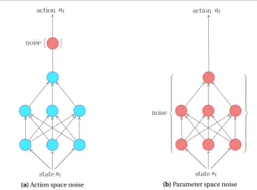
causes a large parameter variance which grows with the number of time steps. Such explo-ration strategies may even damage the robot as random exploexplo-ration in every time step leads to large jumps in the controls of the robot.

The exploration strategy is used to generate new trajectory samplesτiwhich are subsequently evaluated by policy evaluation strategies and used for policy update. Thus, an efficient explo-ration strategy is crucial for improving the performance of policy search algorithms. The ex-ploration strategy can also be categorized based on whether the exex-ploration noise is applied in the action space or the parameter space. Exploration in action space is implemented by adding an exploration noise²udirectly to the executed actions;at=µ(x,t)+²uwhere the exploration

noise is sampled independently for each time step. As a matter of fact, the action noise can be either uncorrelated as Gaussian noise²u∼N(0,σ2I) or correlated as the Ornstein-Uhlenbeck

process²u∼OU(0,σ2). On the other hand, parameter space noise injects randomness directly

into the parametersθ of the policy, altering the types of decisions it makes such that they al-ways fully depend on what the agent currently senses. This exploration noise can either only be added at the beginning of an episode, or, a different perturbation of the parameter vector can be used at each time step.

2.4 Summary

(26)

3 Deep Reinforcement Learning

In this chapter, deep learning and reinforcement learning are combined into what is called Deep Reinforcement Learning (DRL).The value-based methods discussed previously can be represented in a tabular format which is only feasible for state and action spaces with a limited number of states and actions. In cases where bothSandAare big sets, these methods are in-feasible not only due to memory requirements for storing the big value function tables, but also due to the data needed to fill out these tables accurately and the time needed for acquiring that amount of data. Instead of a table representation of the value function, one can use a function that approximates the desired value function. This function approximator is then trained using interactions between agent and environment. Deep reinforcement learning has received a lot of interest among the AI community in the last couple of years where it refers to the use of deep neural networks as function approximators for value functions or policy in an RL framework [19]. The fact that deep reinforcement learning can handle high dimensional state and action space makes it extremely suitable for the purpose of controlling the motion of a mobile robot, the problem under study.

3.1 Artificial Neural Networks

In order to understand neural networks, one first needs to be familiar with the computational units they consist of which are artificial neurons. An artificial neuron is a simple mathematical model that mimics the way biological neurons in the human brain process information [27].

inputs weights

[image:26.595.285.496.420.578.2]

activation function

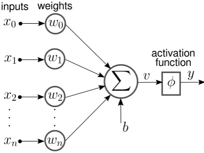
Figure 3.1:Illustration of how an artificial neuron transforms its inputsx0,x1, ...,xnto its outputy.

A neuron is a computational unit that takes as an input a number ofnsignals,x0,x1, ...,xn

and combine them together into a scalar out-put, thus it can be thought of as a mapping function. Each of the input signals are multi-plied by their own weightsw0,w1, ...,wn that

determine how much the individual input signal affects the output of the neuron. These weighted inputs are summed together and a biasb is added before it passes through an activation function, φ that has the effect of applying non-linearity to v. Formally, the output is expressed by the two equations:

v=

n

X

j=0

wjxj+b

y=φ(v)=h(x0,x1, ...,xn)

(3.1)

There are different activation functions that can be used, where the sigmoid function, hy-perbolic tangent (tanh) function, and

(27)

well.

φ(v)= 1

1+e−v (3.2)

φ(v)=max(0,v) (3.3)

An important property of activation functions is that they introduce non-linearity to their in-puts allowing the network to learn any arbitrary functional mappings. In addition, activation functions are differentiable which allow for gradient-based learning methods. Neurons are used to construct networks of connected neurons also known as neural networks. The neu-rons are organized in different layers and these layers are then stacked to build larger networks. There are different types of neural networks for which fully-connected and convolutional neu-ral network are two common types. However, since throughout this thesis, only fully-connected neural networks are discussed, convolutional neural networks are discarded.

3.1.1 Feed-Forward Neural Networks

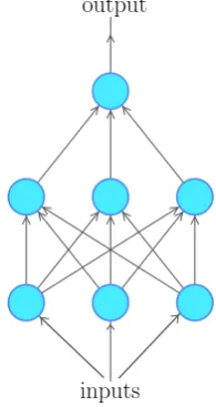
[image:27.595.379.477.370.554.2]

Feed forward neural networks, also called multilayer perceptrons, are the typical deep learn-ing models. A feed forward network is a function that maps an input x to an output y us-ing parameters θ, such as y = f(x;θ). The architecture of a feed-forward neural network usually has three kinds of layers: an input layer, a few hidden layers and an output layer.

Figure 3.2:A fully connected feed-forward neural network with two

hidden layers. The information flows from bottom to top.

The information flows through the network from the input layer to the output layer which computes the fi-nal output through the hidden layers. Unlike recurrent neural networks, there are no feedback connections in which outputs of the model are fed back into itself. A typical fully connected neural network is shown in Fig-ure 3.2.

Training algorithms for deep neural networks are usu-ally iterative, therefore an initial point should be spec-ified to start the training. This starting point affects the number of iterations required for the learning process to be done and the ability of the network to generalize at the end of the training. To update the parameters θi of the network, a loss functionL(θ) is defined that

represents the error between the desired outputy∗_of

the inputxand the actual output y obtained by per-forming a forward path through the network using the current parameters. The gradient of the loss function

∇θL(θ) is computed and the parameters are readjusted

in the opposite direction of the gradient by propagat-ing backward in the network. This algorithm is refer-eed to asbackpropagation algorithm that applies

re-cursively the chain rule to compute the gradients, starting from the output layer all the way back to the input layer. In the recent years, stochastic gradient descent has been a popular choice for training the weights of a neural network. A few improved variants of stochastic gra-dient descent has also been proposed, like ADAM [28]. The advantage of using ADAM method over standard stochastic gradient descent is that it can vary the learning rates based on the dis-tribution of the training data. This reduces the need for careful choice of a learning rate which in turn allows the algorithm to converge faster.

(28)

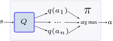
evaluates the quality of taking this certain action from that state in the form of an action value function. The second way is to pass only the state as the input to the network and then evaluate the quality of taking any of the all feasible actions from this state. In this case, the output of the network is composed of as many neurons as the number of actions. Based on the estimated action value-functions, the algorithm selects one of the actions based on the deployed policy, i.e, in case of an²-greedy policy, the algorithm is going to select the action with highest value function with a probability of (1−²)%. Here it is worth mentioning that the second way is only possible in case there is a discrete number of actions since the Q-value is estimated for every action.

(a)The action and state are used as inputs to the network and the quality of taking this action from

that state is determined in form of a Q-value.

(b)The state represents the input of the network

[image:28.595.100.468.206.390.2]

and the Q-values are estimated for all feasible actions from this state.

Figure 3.3:A graphical representation of neural networks as function approximators in reinforcement learning context [29].

As a matter of fact, neural networks can also serve as a function approximator for a parametric policy in case of a policy search based reinforcement learning as will be discussed later in this chapter where the input of the network is the current state of the robot and the output is the mapped action.

In the next section, it is shown how to use neural networks as function approximators for Q-values in reinforcement learning context.

3.2 Deep Q-Networks

Q-Learning, discussed in section 2.3.1.2, has been a widely used algorithm for model-free re-inforcement learning. However, it was shown that utilizing neural networks as function ap-proximators, to approximate the optimal action value functionQ(s,a;θQ)≈Q∗(s,a), directly to Q-learning algorithms without further modifications leads to an unstable behavior and the convergence is no longer guaranteed [30] and thus, most applications of Q-learning were lim-ited to tasks with small state spaces. The main cause of this issue is that when using neural net-works for reinforcement learning, it is assumed that the samples are independently distributed. However, this is not the case when the samples are generated sequentially since they are tem-porally correlated which results in high variance in the estimation. To tackle this problem an experience replayis introduced to break the temporal correlation between the consecutive tran-sitions where the agent’s experience at each time stepet= 〈st,at,rt,st+1〉is stored in a replay bufferD₌{e1,e2, ...,eN} with a finite sizeN. At each time step, a fixed number of samples, a

mini-batch, is extracted randomly from the replay buffer and used to train the network. When the replay buffer is full, the oldest samples were discarded meaning that the replay bufferD

(29)

used to minimize the TD-error squared. The learning of the value-function in deep reinforce-ment learning is based on the adjustreinforce-ment of the neural network weights by minimizing the loss function, which corresponds to the mean squared error between the TD target and the current value function Li ³ θQ i ´

=Es∼ρπ(.),a∼π(.)        

Q³st,at;θQ_i

´

−yi

| {z }

TD error     2    (3.4)

whereyi=r(st,at)+γmax at+1

Q³st+1,at+1;θQ_i

´

is the target at iterationi,π(a|s) is the behaviour policy andρ_π(.)is the distribution of states under policyπ(a|s). To minimize the loss function, the gradient of the loss function is computed with respect to the weights and is given by

∇_θQ i

L³θQ_i ´=Es∼ρπ(.),a∼π(.) ·µ

Q³s,a;θQ_i ´−r(st,at)−γmax_a

t+1

Q¡

st+1,at+1;θQ

¢ ¶

∇_θQ i

Q³st,at;θQ_i

´¸

(3.5)

The parametersθare updated using the stochastic gradient descent of the loss function such that

θi+1=θi−α∇_θQ iL ³ θQ i ´ (3.6)

As a matter of fact, DQN is is an off-policy model-free algorithm where the agent learns the Q-value function, while following a different behavior policy that provides sufficient exploration of the domain space. In practice, the behaviour policy is generally selected by an²-greedy strategy. In [5], it is shown that implementing equation (3.4) directly results in divergence in many cases. The reason is that the updatedQ(s,a|θQ) is also used with the same weights in calculating the TD targetyt which makes the optimization appears to be chasing its own tail

resulting in instability. One possible solution is to introduce a second network calledtarget neural network that is proposed in [31] to calculate target Q-values Q0(s,a|θQ0) where the target network parametersθ0are only updated with the Q-network parametersθevery certain number of steps. The target-network and the Q-network share the same network architecture, but only the weights of the Q-network are learned and updated. A graphical representation of the DQN approach is shown in Figure 3.4

[image:29.595.206.399.517.588.2]

arg max

Figure 3.4:Architecture of DQN where the Q-Network outputs an estimate of the action-value function

for each action. Subsequently, the policy_πchooses the action with the highest value.

(30)

Algorithm 3Deep Q-Network

Initialize action value functionQ(s,a;θQ) with random weights. Initialize a replay bufferDwith sizeN.

Initialize target action value functionQ0(s,a;θQ0) withθQ0=θQ. for allepisodedo

Initializes1 repeat

for each steptin an episodedo

Choose an actionat∈Ausing²-greedy strategy.

Execute actionat, observe rewardrt+1and new statest+1. Store transition〈st,at,rt,st+1〉in replay bufferD.

Sample random mini-batch of transitions〈si,ai,ri,si+1〉fromD. ifsi+1is terminalthen

yi=ri

else

yi=ri+γmax at+1

Q0(st+1,at+1;θQ

0 )

end if

Train the Q-network on (yi−Q(si,ai;θQ))2using (3.5).

end for untilterminated end for

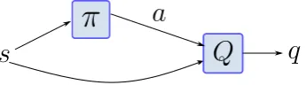
The one major drawback of the above algorithm is the need to calculate the maximum over actions and this prohibits the use of of the above algorithm for tasks with continuous actions spaces. To deal with continuous action spaces, an actor critic algorithm was developed which uses the Q-function as the critic and updates the policy using the Deterministic Policy Gradient discussed in the following sections.

3.3 Actor-Critic Algorithms

It is possible to combine value functions with an explicit representation of the policy, resulting inactor-criticmethods. Actor-critic methods are TD methods which store the policy explicitly. The policy is known as the actor since it predicts the action in a given state. The value function acts as the critic since it evaluates the policy based on the temporal difference error. The policy is updated based on this critic. The actor critic method is mostly on-policy, but off-policy actor critic have been introduced in the literature [32]. Actor critic algorithms can either store the actor and critic in a tabular form or can use function approximators, which is the case with most robotic applications. When using function approximators, the policy is updated similar to policy search methods, except that the critic decides the direction of gradient ascent instead of the expected return. The stochastic policy gradient theorem [33] defines the gradient of the expected return,∇θπJ(π_θ), using the likelihood-ratio trick explained beforehand in section

2.3.2.1, as

∇θπJ(π_θ)₌

Z

Sρ

π_(s)Z

A∇θ

ππ_θ¡a_|s;θπ¢Qπ(s,a;θQ)dads

=

Z

Sρ

π_(s)Z

Aπθ