Hybrid algorithms for subgraph pattern queries in graph databases

(1)

warwick.ac.uk/lib-publications

Original citation:

Katsarou, F., Ntarmos, N. and Triantafillou, P. (2017) Hybrid algorithms for subgraph pattern

queries in graph databases. In: 2017 IEEE International Conference on Big Data (IEEE BigData

2017), Boston, MA, USA, 11-14 Dec 2017

Permanent WRAP URL:

http://wrap.warwick.ac.uk/93846

Copyright and reuse:

The Warwick Research Archive Portal (WRAP) makes this work by researchers of the

University of Warwick available open access under the following conditions. Copyright ©

and all moral rights to the version of the paper presented here belong to the individual

author(s) and/or other copyright owners. To the extent reasonable and practicable the

material made available in WRAP has been checked for eligibility before being made

available.

Copies of full items can be used for personal research or study, educational, or not-for profit

purposes without prior permission or charge. Provided that the authors, title and full

bibliographic details are credited, a hyperlink and/or URL is given for the original metadata

page and the content is not changed in any way.

Publisher’s statement:

© 2017 IEEE. Personal use of this material is permitted. Permission from IEEE must be

obtained for all other uses, in any current or future media, including reprinting

/republishing this material for advertising or promotional purposes, creating new collective

works, for resale or redistribution to servers or lists, or reuse of any copyrighted component

of this work in other works.

A note on versions:

The version presented here may differ from the published version or, version of record, if

you wish to cite this item you are advised to consult the publisher’s version. Please see the

‘permanent WRAP url’ above for details on accessing the published version and note that

access may require a subscription.

(2)

Hybrid Algorithms for Subgraph Pattern Queries in Graph Databases

Foteini Katsarou School of Computing Science

University of Glasgow, UK [email protected]

Nikos Ntarmos School of Computing Science

University of Glasgow, UK [email protected]

Peter Triantafillou Department of Computer Science

University of Warwick, UK [email protected]

Abstract—Numerous methods have been proposed over the

years for subgraph query processing, as it is central to graph analytics. Existing work is fragmented into two major categories. Methods in the filter-then-verify (FTV) category

first construct an indexof the DB graphs. Given a query, the

index is used tofilterout graphs that cannot contain the query.

On the remaining graphs, a subgraph isomorphism algorithm

is applied to verify whether each graph indeed contains the

query. A second category of algorithms is mainly concerned with optimizing the Subgraph Isomorphism (SI) testing process (an NP-Complete problem) in order to find all occurrences of the query within each DB graph, also known as the matching problem. The current research trend is to totally dismiss FTV methods, because SI methods have been shown to enjoy much shorter query execution times and because of the alleged high costs of managing the DB graph index in FTV methods. Thus, a number of new SI methods are being proposed annually.

In the current work, we initially study the performance of the latest SI algorithms over datasets consisting of a large number of graphs. With our study, we evaluate the algorithms’ performance and we provide comparison details with former studies. As a second step, we combine the powerful filtering of a top-performing FTV method, with the various SI methods, which leads to the best practice conclusion that SI and FTV shouldn’t be thought of as disjoint types of solutions, as their union achieves better results than any one of them individually. Specifically, we experimentally analyze and quantify the (posi-tive) impact of including the essence of indexed FTV methods within SI methods, showing that query processing times can be significantly improved at modest additional memory costs. We show that these results hold over a variety of well-known SI methods and across several real and synthetic datasets. As such, hybrids of the type reveal a missing opportunity and a blind spot in related literature and trends.

Keywords-Graph DB, graph query processing, subgraph

isomorphism

I. INTRODUCTION

Graphs are ideal for representing complex entities and their relationships. Finding the occurrence(s) of a pattern graph within the various graphs in a graph DB is essential

to graph analytics. In subgraph querying, given a pattern

graph (query) and a graph DB, we want to know whether the query graph is contained in each graph (the decision problem) and/or find all its occurrences within one or more stored graphs (the matching problem). Subgraph querying entails the NP-complete subgraph isomorphism problem (abbreviated as sub-iso). Over the years, subgraph querying

has received and continues to receive a lot of attention, as is evident by the numerous new methods proposed annually. Additionally, four recent experimental analysis papers ([1]– [4]) compare and stress-test the proposed methods and pro-vide interesting insights about the performance of various so-lutions. Related work is segregated in two major categories:

the filter-then-verify (FTV) and the subgraph isomorphism

(SI) methods. Specifically, FTV methods mainly focus on

filtering out graphs that do not contain a query graph as an answer and then employ a “standard” SI algorithm for verification, whereas for SI methods indexing/filtering is usually neglected in favor of better/faster SI heuristics. The more recent works, e.g. [3], [5], [6], dismiss the FTV methods with the claim that the fast sub-iso test of the SI methods significantly outperforms the index-based FTV methods. Thus, all recently published methods follow the SI paradigm.

In the current work, our goal is to identify the best practices for processing subgraph pattern queries. In turn this rests on two pillars: The first is a head-to-head com-parison and evaluation of the state-of-the-art SI methods. Our findings will allow a direct comparison with [3] for the common algorithms, but will also include interesting insights for 2 notable and high performing SI methods proposed after the publication of [3]. Second, and more importantly, armed with the knowledge of the above conclusions, we investigate best practices for subgraph pattern querying in graph DBs by combining the main assets of the FTV and SI methods to derive hybrid FTV-SI methods. Perhaps surprisingly, no prior research has considered to study the impact of hybrid FTV-SI solutions, whereby the benefits of a top-performing graph DB index are combined with the fast sub-iso heuristics offered by the SI methods. This paper shows that such approaches can be very beneficial and suggests how to address the key shortcomings of such hybrid solutions.

(3)

graphs? (4) What are the time/space trade-offs involved in this process? (5) Finally, the dominant question is “can we achieve significant speedups by using hybrid solutions and quantify the speedups given memory and time constraints for the index?” With a typical graph dataset consisting of many large graphs and the actual answer set consisting of a small portion of graphs, with this work we show that large performance gains are possible. We employ three real and a synthetic dataset generated with GraphGen. Finally, we consider five popular, recent and efficient SI methods for our evaluation and a top-performing filtering approach from an FTV method to construct our best practice hybrids.

II. BACKGROUND

A. Related work

Related work examines two versions of the subgraph

querying problem: the decisionand the matching versions.

In the decision version, given a DB of many (typically small)

graphs and a query/pattern graph q, the method decides

whetherqis contained in any graph in the dataset and returns

the IDs of those graphs. In the matching version, the method

finds all embeddings of the query graph q in a typically

large, stored graph gor in each graph of a graph DB.

Proposed methods can be classified as filter-then-verify

(FTV) or directsub-iso(SI). Popular FTV methods include

[7]–[15]. These methods need to first build an index. To do so, stored graphs are decomposed into features which are then indexed, along with graph-ID lists; i.e., lists of graphs that contain the feature. The features can be paths, trees, subgraphs, cycles or a combination of the above and are ob-tained either through an exhaustive enumeration or frequent mining. Query processing consists of two stages. In the first,

filtering stage, query graphs are similarly decomposed into

features; DB graphs that do not contain one or more of these features definitely do not contain the query and are pruned away. On the remaining graphs, an intersection of

the graph-ID lists is performed to form thecandidate set. In

the verification stage, the query graph is tested for sub-iso

against each graph in the candidate set to produce the final answer set. Proposed methods try to optimize 4 criteria: (i) indexing time, (ii) index size, (iii) query processing time and (iv) candidate set size. The methods’ design options reflect on their scalability, i.e., the ability of constructing the index in reasonable time and size and answering queries in reasonable time. FTV methods are extensively discussed in [1], [2]. [2] concluded that Grapes[9] and GGSX[7] are the best solutions in terms of index construction time, query processing time, and scalability limitations. It was also showed that both Grapes and GGSX enjoy similar filtering power for datasets consisting of relatively small graphs. However, when the graph sizes increase, Grapes outperforms GGSX in filtering power.

The focus of SI methods, is not to filter out graphs in the dataset that definitely do not contain the query as

an answer, but for each DB graph (i) to locate the best candidate vertices to expedite the sub-iso test, and (ii) to decide the optimal join plan to follow; i.e., the sequence in which the query vertices will be matched to those of the stored graph. Thus, proposed SI methods, apart from the sub-iso heuristic algorithm, additionally contain a pre-processing/indexing step where they maintain a feature-based index, along with vertex label lists and additional information to facilitate the sub-iso test. Popular SI methods include [11], [16]–[19]. During query processing, they apply different heuristics and define different join operations to match the query. A number of such methods were presented and compared in [3], concluding that (i) although there was no single algorithm to outperform all others in all occasions, GraphQL[18] was the only one that managed to complete all tested query workloads; (ii) GraphQL and sPath[17] showed very good performance; but also that (iii) all existing algorithms have weaknesses in the way they apply their join selection and pruning heuristics, leading to the need for new SI methods. Following the publication of [3], several sub-iso tests were proposed. TurboIso[5] rewrites the query by merging vertices that share the same label and neighborhoods. BoostIso[20] applies the aforementioned rewriting technique to the stored graph and dynamically reduces the duplicate computations. Thus, BoostIso claims it can accelerate all proposed sub-iso techniques. CFL-Match[16] applies decomposition of the query in dense subgraph and forest and unlike other methods, CFL-Match processes the dense subgraph first. Finally, Peng et al.[21] decompose the query in adjacent edge pairs or star-style patterns and propose an Edge Join algorithm.

A recent work [4] provided key insights about the perfor-mance of both FTV and SI methods. Specifically, [4] showed that all existing sub-iso algorithms suffer from straggler-queries; i.e., queries whose processing time is many orders of magnitude worse compared to the rest. Secondly, that isomorphic queries can have widely and wildly different ex-ecution times. Thus, straggler queries may have isomorphic instances which are not stragglers. Finally, that stragglers are algorithm-specific, i.e. a straggler-query on one algorithm can be a typical query on the other algorithm. These findings

yielded theΨ-framework, which executes in parallel threads

of different query rewritings and/or alternative algorithms to achieve large performance gains on both research camps.

(4)

for subgraph queries for FTV and SI methods. Similarly,

PatternTreeISO[26] utilizes pattern correlations of preceding

queries to expedite subgraph isomorphism for subsequent ones. [10], [27] perform subgraph matching, but with the ad-ditional support for wildcards and/or approximate matches, and Lin et al.[28] address the problem of generalized subgraph query processing. Finally, Semertzidis et al.[29] considered pattern queries over time-evolving graphs.

Contributions: We evaluate top-performing SI methods

against datasets consisting of a large number of graphs to provide insights about their performance. Our findings com-pare with [3] for the 3 common algorithms and complement it with inclusion of 2 notable SI methods proposed after the publication of [3]. In parallel, we thoroughly investigate the current community wisdom which tends to dismiss FTV methods based on the fact that the fast sub-iso test of the more recent SI methods can significantly outperform the index-based FTV methods [3], [5], [6]. This is indeed a claim we have verified as well: when comparing a fast SI algorithm (even if not the fastest one, such as GraphQL) against a top-performing FTV algorithm (such as Grapes) for queries run over a single graph DB, SI methods are the winners. However, this fact requires further analysis which has not as of yet been performed. Note that: (1) No analysis for the reasons of this fact has ever been provided. (2) SI methods also essentially develop and utilize indexes for pruning the search space during matching; no one has ever really provided any insights as to how costly in time and in memory space this is. And, combined with (1) above, (3) No evidence exists so far that relates the efficacy of FTV-indexes versus SI-FTV-indexes in terms of reducing the search space. Finally, FTV algorithms utilize both a filtering and a verification stage. Hence, if FTV-type indexing is more powerful than SI-type indexing, this implies that the sub-iso heuristics of SI methods must significantly outperform the verification of FTV methods. Therefore, combining the FTV pruning power with the great efficiency of SI algorithms appears to be a promising avenue for new performance gains. So, the real issue becomes to (4) Investigate and quantify what are the expected performance gains of hybrid FTV-SI solutions. With this paper, we will tackle the above issues and we will show that dismissing completely indexed FTV methods leads to missing an opportunity for significant performance gains, revealing thus a blind research spot. This we hope will motivate new research into hybrid FTV-SI combinations and new indexes and/or new sub-iso heuristic algorithms for such hybrids.

B. Definitions

Definition 1 (Graph): A graph G= (V, E, L)is defined

as the triplet consisting of the set V = {vi}, i = 1, ..., n

of vertices of the graph, the set E ⊆ {(v, u) : v, u ∈ V}

of edges between vertices in the graph, and a function L:

V|E → L assigning a label l ∈ L (L being the set of all

possible labels) to each vertexv∈V and each edgee∈E.

Definition 2 (Graph Isomorphism): Two graphs G =

(V, E, L) and G0 = (V0, E0, L0) are isomorphic iff there

exists a bijectionI:V →V0that maps each vertex ofGto a

vertex ofG0, such that if(u, v)∈E then(I(u), I(v))∈E0,

L(u) =L0(I(u)),L(v) =L0(I(v)), and vice versa.

Definition 3 (Subgraph Matching Problem): Given a set

of graphsD=G1, ..., Gn, and a query graphq, the subgraph

matching problem determines all graphs Gi ∈D such that

q⊆Gi and finds all the occurrences ofqwithin eachGi.

III. EXPERIMENTALSETUP

A. Algorithms

We opted for methods (i) whose code is publicly available or made available to us by the authors upon request, so any conclusions would not be implementation dependent and (ii) that were well recognized as well performing. From the FTV methods, we chose Grapes[9], which was declared top-performing in terms of indexing time, query processing time, false ratio and scalability in [2]. Reagrding the SI methods, we selected GraphQL[18], sPath[17], QuickSI[11], TurboIso[5], and BoostIso[20] over TurboIso. With respect to CFL-Match[16]: we did not employ the algorithm as its authors did not respond to our request for their code.

1) FTV method: Grapes[9] (GR) indexes simple paths of

up to a maximum length, along with location information, in a trie, enumerated in DFS order. GR can work with multiple threads for both indexing and query processing. In query processing, maximal paths of the query are extracted to form the query index which is matched against the DB index, pruning away unmatched branches. Then, the search space is further pruned using frequencies of the indexed features and the maintained location information is used to extract the relevant connected components of DB graphs, against which sub-iso testing is performed using VF2[30].

2) SI methods: In GraphQL[18] (GQL), the vertex labels

along with the neighborhood signatures, which capture the

labels of neighboring nodes in a radiusiin lexicographical

order, are indexed. In the subgraph matching phase, the algorithm starts by retrieving all possible matches for each node in the pattern. Then, 3 rules are applied in order to prune the search space. First, the indexed vertex labels and neighborhood signatures are used to prune away infeasible matches. Then a pseudo sub-iso algorithm is applied

itera-tively up to level l; i.e., for every pair of possible

graph-query vertex matches, the nodes adjacent to the graph-query node should be matched to the corresponding neighbors of the graph. Finally, the algorithm optimizes the search order in the query before proceeding with the actual sub-iso test,

which in turn consists of a number ofjoinsof the candidate

(5)

sPath[17] (SP), similarly to GQL, also maintains a neigh-borhood signature encoding where shortest paths are orga-nized in a compact indexing structure. In order to reduce space, shortest paths are not really maintained, but are decomposed in a distance-wise structure. In the query pro-cessing, the query is initially decomposed in shortest paths that are then matched to the shortest paths from each DB graph. From all possible candidate shortest paths, those that (i) can cover the query and (ii) provide good selectivity, i.e., minimize the estimated result-set size of each join operation, are selected as candidates. An edge-by-edge verification is used to perform the sub-iso test against the latter.

QuickSI[11] (QSI), gives priority to the vertices with infrequent labels and infrequent adjacent edge labels. In the indexing phase, QSI pre-computes the frequencies of labels and edges and uses them to compute the “average inner support” of a vertex or an edge; i.e., the average number of possible mappings of the vertex or edge in the graph, which is later used in the graph matching process to assign weights on the edges of the query graph and construct a rooted minimum spanning tree (MST). In case of symmetries, edges are added in such a way that will make the MST denser. The order in which vertices are inserted to the MST defines the order in which they are then matched in the sub-iso test.

TurboIso[5] (TI), utilizes 2 data structures as its index: (i) an inverse vertex label list that allows easy access to the vertices that share the same label, and (ii) a list of adjacent vertices for every vertex. TI defines the Neighborhood Equivalent Class (NEC) as the class of vertices that share the same structure; i.e., the same labels. In the query processing, for a given query a starting (root) vertex is chosen based on a ranking function that favors low label frequencies and high node degrees and the query is rewritten to the equivalent NECtree. Initiating from the root query vertex, TI identifies candidate regions (CR) to the stored graph by performing a DFS search on the query’s NECtree. The matching sequence for the query vertices is again chosen as to minimize the intermediate candidate results. However, TI defines a better matching order because of the more precise CR estimation. Specifically, TI exploits the paths of the NECtree from the starting vertex to every leaf node of the NECtree, and calculates the cardinalities of their CR. Based on that, a matching order is defined in ascending order to the vertices of the NECtree.

BoostIso[20] (BI) can be applied on top of every proposed back-tracking algorithm and is based on the use of 4 types of relationships: (i) syntactic containment (SC), (ii) syntactic equivalence (SE), (iii) query-dependent containment (QDC), and (iv) query-dependent equivalence (QDE). The first 2 are used to transform the stored graph to the adapted hypergraph

Gsh, whereas the rest further reduce duplicate computations

in query processing. Empirically, SC is evident in the case that 2 nodes have the same label and the neighboring set of nodes on the second node is contained in the first node. In

SE, 2 nodes share the same label and the same neighboring set of nodes. QDC and QDE rule similar conditions to SC and SE between the nodes of the query and the nodes of the stored graph. As a pre-processing step, BI employs graph adaptation to transform a stored graph to the adapted hypergraph, by utilizing the Syntactic Equivalence Class (SEC). Note that, vertices in the same SEC form a clique or are pairwise adjacent (they are either 1-step or 2-step reachable from each other respectively), and thus the adapted hypergraph captures the structure of the original graph along with the SE and SC relationships between vertices. In the query processing, BI searches for hyperembeddings of the query graph in the adapted hypergraph which are translated to embeddings. Duplicates can be further reduced using QDC and QDE relations along with the SC and SE relations. For our experiments, we employ BI over TI (BTI for short).

B. Setup

All the experiments were conducted on a Windows 7 SP1 host, with 2 Intel Xeon E5-2660 CPUs (2.20GHz, 20MB cache) with 8 cores/16 vcores per CPU, 128GB of RAM, and 3.5TB disk. We ran our experiments individually and one at a time to avoid any interference across runs.

For GR we used the implementation provided by its authors. For GQL, SP, and QSI, we used the implementation provided by [3]. For TI we obtained the binary code from the authors and for BTI we obtained the source code from

GitHub1_{. We used the default values for the input parameters}

of the compared algorithms, as they were defined by their respective authors in the relevant publications and/or in their implementation code. Specifically:

• For GR, we enumerated paths of up to size of 4. We

used 1 and 4 threads; results for executions with 1 (resp. 4) threads are denoted by GR/1 (resp. GR/4).

• For GQL, we used a refined level of iterations of

pseudo-subgraph isomorphism r= 4.

• For SP, we used a neighborhood radius of 4 and

maximum path length 4.

• TI and BTI do not require any input parameter.

How-ever, for TI we were able to execute queries of only up to 25 vertices, due to an inherent limitation in the executable provided to us (and we were unable to amend this because we were only provided with the binary).

• For all SI methods the number of searched embeddings

of the pattern graph in the stored graph is capped at 1000; i.e., after finding the first 1000 matches, the algorithms terminate.

C. Datasets

Table I summarizes the characteristics of the employed datasets. PDBS, PCM and PPI are 3 real datasets that

(6)

PDBS PCM PPI Synthetic

Dataset

# graphs 600 200 20 1000

#disconnected 360 200 20 0

graphs

#labels 10 21 46 20

Per

Graph

Avg #nodes 2939 377 4942 1100

StdDev #nodes 3215 186.7 2648 483

Avg #edges 3064 4340 26667 12487

Avg density 0.0007 0.0612 0.0022 0.020

Avg degree 2.06 23.01 10.87 24.5

[image:6.612.330.535.73.228.2]

Avg #labels 6.4 18.9 28.5 20

Table I

DATASET CHARACTERISTICS

were previously used in [2], [9]. PDBS and PCM represent chemical compounds comprising of 600 and 200 graphs respectively, whereas PPI represents 20 proteprotein in-teraction networks. The majority of existing real datasets comprise of relatively small and sparse graphs, and thus in the lack of real datasets publicly available that preserve the required properties (i.e., many large graphs), we additonally employ a synthetic dataset of 1000 graphs generated with GraphGen[8] a standard tool for constructing datasets suit-able for graph mining techniques and subgraph queries, as it allows the parametrisation of various parameters of interest; namely, number of graphs, average number of nodes and density per graph, number of labels in the dataset, etc.

D. Query Workloads

To generate each of the queries, we select a graph from the dataset uniformly and at random, and from that graph we select a node uniformly at random. Starting from said node, we generate a query graph by incrementally adding edges chosen uniformly at random from the set of all edges adjacent to the resulting query graph, until the desired size is reached. For PDBS and PCM, we used queries of size 20 and 24 edges. For PPI, we used queries of size 16, 20, 24, and 32 edges. For the synthetic dataset, we used queries of size 24, 32 and 40 edges. For every query size we used 200 queries for PDBS and PCM and 100 queries for PPI and the Synthetic dataset. Finally, as we already mentioned, we

were unable to execute queries >25 vertices on TI. Thus,

in the presentation of our results in the subsequent figures for TI we only present results for queries up to 24 edges, as to qualify with this restriction.

IV. INDEX CONSTRUCTION

As we already mentioned, both FTV and SI methods rely on an index but to fulfill different purposes. For the FTV methods, the index construction facilitates the pruning of graphs in the dataset that definitely do not contain the query graph as an answer. For the SI methods the index purpose is to locate the candidate vertices on the stored graph to expedite the sub-iso test. Thus, SI methods require less time and space to construct and store their index respectively.

1 10 100 1000 10000

time (s)

GQL SP

QSI TI

BTI GR/1

GR/4

Synthetic PPI

PCM PDBS

(a) Indexing time

1 10 100 1000 10000 100000

size (MB)

GQL SP QSI TI BTI GR

Synthetic PPI

PCM PDBS

[image:6.612.61.290.73.188.2]

(b) Index size

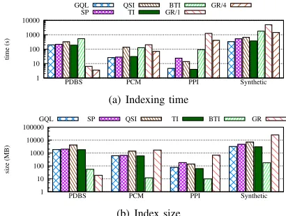
Figure 1. Indexing time and size

Fig. 1 presents the results from the index construction phase for all datasets and used algorithms. Please note that for GR, the index size is independent of the number of threads and thus only one bar/line is used in corresponding fig. 1(b) for this algorithm. Among the SI methods, we notice

the following trend in the index sizes:SizeQSI> SizeSP >

SizeGQL > SizeT I > SizeBT I and this trend is also

followed by the indexing time, with sole exception of BTI where the indexing time is comparable to that of QSI. In the majority of algorithms, this is somewhat expected because of the structures used by each algorithm to maintain the index. Specifically, based on the code we had available, we note that GQL and SP along with the additional information they require to store their index – i.e. labels of neighbouring

nodes in radiusishorted in lexicographical order for GQL,

and shortest paths for SP – they also store the actual graphs

in a convenient format as presented in TI (§IV). Our results

come in agreement with [3] for GQL and SP but not for QSI. Finally BTI’s index consists of 2 distinct files that store the

hypergraph and containment graph (as described in§III-A)

and even though their size is already small enough, it could be diminished if index files were in a binary format.

(7)

0 20 40 60 80 100

avg % graphs

GQL_CSS SP_CSS GR_CSS ASS

Synthetic PPI

PCM PDBS

(a) Candidate and answer sets for all algorithms

0 0.2 0.4 0.6 0.8 1

false positive ratio

GQL SP GR

Synthetic PPI

PCM PDBS

[image:7.612.68.275.72.236.2]

(b) False Positive Ratio

Figure 2. Pruning Power

V. FILTERING POWER

To quantify the filtering power, we utilize 2 different metrics: (1) the percentage of graphs that constitute the candidate set for each algorithm, before proceeding with the final sub-iso test, (2) the false positive ratio, defined as:

F P R= 1 |Q|

X

q∈Q

|C{q}| − |A{q}|

|C{q}| (1)

where|·|denotes set cardinality,Qis the set of all queries in

each query workload, andC{q}andA{q}are the candidate

set and answer set respectively for query q, with A{q} ⊆

C{q}. We note thatF P R= 0means that the candidate set

is exactly the same as the answer set and F P R = 1 that

although some/all of the graphs in the dataset belong in the candidate set none of them is found to be an answer in the query, i.e. the answer set size is 0.

Fig. 2 presents the results for the pruning power of used algorithms. CSS stands for Candidate Set Size and ASS stands for Answer Set Size. QSI, TI, and BTI are not included in the presented results as they do not perform any filtering and proceed directly to the sub-iso test. GR provides the same filtering power independently of the number of threads that are executed and thus on the corresponding figures we do not distinguish the results. For comparison purposes, we report the percentage of graphs that constitute the avg ASS along with the percentage of graphs that constitute the avg CSS for each algorithm in fig. 2(a).

Different number of graphs were filtered out by all 3 different methods. Although it is not presented in the above figures, the filtering power of the SI methods is slightly improved as the query size increases and the same effect holds for GR. In the majority of cases GR was able to filter out at least double the amount of graphs compared to GQL and SP, leading to candidate sets very close to the actual answer set. This is also evident in the low FPR. However,

as we already discussed in§IV, GR’ filtering comes at an

extra cost of a much larger index to store and more time

1 10 100 1000 10000 100000 1x106

avg query exec time (ms)

GQL SP QSI TI BTI

Synthetic PPI

[image:7.612.332.533.73.138.2]

PCM PDBS

Figure 3. Avg query exec time (ms) of SI methods

to construct, with the sole exception of PDBS. SP, that constructs a slightly more elaborate index compared to GQL, was also able to achieve an up to 10% better filtering than GQL. A very interesting observation is the fact that in very rare cases the graphs that were filtered out by the SI methods were not always a subset of the graphs filtered out by GR.

This occurred in<1% of a graph-query pair and was more

evident when increasing the query size. Finally, we note that it is important to observe the FPR in combination with the CSS and ASS. To showcase this, we note that although PDBS is the only dataset where the avg CSS are among the biggest for all 3 algorithms reported, the corresponding FPR are the lowest for all datasets because of the high ASS.

VI. PERFORMANCE OFSIMETHODS

The current tendency in recent work is to totally dismiss FTV methods with the claim that the fast sub-iso test of the SI methods outperforms the index-based FTV methods. Before proceeding with further investigating this claim, we provide in fig. 3 a head-to-head comparison of the avg query execution time of SI algorithms across all datasets. Please

note that because of the restriction mentioned in§III-B, for

TI and for PPI and Synthetic dataset only results with queries

≤24edges are presented.

As it can be seen, there is no winner algorithm across all datasets. This finding comes in agreement with [3]. TI and BTI, the newest additions in the set of SI algorithms, are favored particularly in datasets consisting of a small number of labels because of the smart rewritings applied on the query graph (and on the stored graph in the case of BTI). The least promising one is QSI, but outperforms BTI on PPI where the number of distinct labels is more abundant. Finally, although we do not present results for different query sizes because of space restrictions, we note that as we increase the query size, query processing becomes harder for all algorithms, with the exception of PDBS and PCM where there are no significant differences for different query sizes.

VII. THE HYBRIDFTV-SIMETHOD

(8)

in §III-A1) and till the stage of forming the candidate set. Subsequently, for those graphs that pass the filtering stage we use GQL/SP/QSI/TI/BTI, instead of GR’s default (and expensive) VF2 sub-iso test. Since an extra filtering step is introduced (namely, the filtering from GR), it is worthwhile evaluating, analysing, and quantifying the effect of the cost to perform this additional on-line filtering on the overall achievable performance. As GR was originally designed to

work in parallel, we utilize (·)/N to denote the in use

number of threadsN for GR-[GQL/SP/QSI/TI/BTI] as the

FTV-SI combination of algorithms. In this section we utilize only one thread; additional parallelism will be discussed in the following section. Last, for the rest of the discussion, we assume that the indices are already loaded into main memory once at the beginning of the execution.

A. Performance Metrics

For every query against a dataset of graphs, we measure

the execution time. For the SI methods the execution time

includes the time for constructing the index of the query, the matching of the query’s index to the databases’ index (where applicable) and the time required to perform the sub-iso test. For our proposed hybrid FTV-SI solution the execution time includes (i) the time required to perform the filtering of GR

as described in §III-A and (ii) the execution time of the in

use SI method for the graphs that passed the filtering stage.

Let qi be a given query. Let also tMi be the execution

time of qi over method M and tGRi −M be the execution

time ofqi over the hybrid combination of GR with method

M over all the graphs in the dataset. In order to evaluate the

performance of this combination, we utilize the speedup∗

metric defined as: t

M i

tGR_i −M. speedup

∗ _{represents what we}

lose in performance if we choose the original method over

the various alternatives; i.e.,speedup∗equals the maximum

attainable speedup over the original method, if we chose the best of the examined alternatives.

When comparing two sets of measurements A = {Ai}

andB={Bi}, we can compute their avg ratio in two ways:

• Workload-Level Aggregation (WLA), given byavgi(Bi)

avgi(Ai).

WhenAandBcontain query response times, the WLA

computation would give the improvement in the overall average execution time. This metric is important from

the system perspective as it encapsulates the overall

performance change.

• Query-Level Average (QLA), computed asavgi

Bi

Ai

. When applied to query processing times, the QLA computation would give the average of per-query

im-provements. This metric isuser-centricin the sense that

each user cares what the performance improvement for his query is using different methods.

In both cases, avgi(Xi) is the average over all items Xi

in the set X. Based on this distinction, the aforementioned

speedup∗ metric can have a QLA or WLA version, denoted

0 1 2 3 4 5 6 7 8 9 10

avg speedup*

QLA

(GR-GQL)/1 (GR-SP)/1

(GR-QSI)/1 (GR-TI)/1

(GR-BTI)/1

Synthetic PPI

PCM PDBS

(a) Avgspeedup∗QLA

0 1 2 3 4 5 6

avg speedup*

WLA

(GR-BTI)/1

Synthetic PPI

PCM PDBS

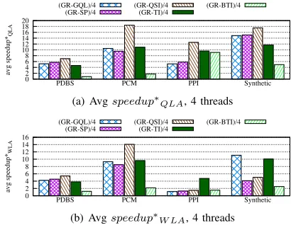
[image:8.612.330.534.73.232.2]

(b) Avgspeedup∗W LA

Figure 4. Avgspeedup∗

QLA&speedup∗W LA

with a matching subscript; e.g., speedup∗QLA. These two

variants also carry over to other computations; for example,

the standard deviation of the ratio ofAandBwould be

com-puted as stdDevi(Bi)

stdDevi(Ai) under WLA, and as stdDevi(Bi/Ai) under QLA. However, unless stated otherwise, we shall use QLA and WLA to denote averages. To highlight the importance of distinction between QLA and WLA metric we note that the workload-based metric in itself (unavoidably) is not entirely reliable as such metrics provide only one point of view: that of the system. However, to the average user, this is not particularly informative. To her the question is what is the best method for her query and by how much; or, put differently, what is the probability that a given method will perform best for her query. This has the affect of treating all queries (and thus users) equally, despite the time taken by each query to execute. Such query-based metrics have unfortunately so far escaped all related work.

B. Performance Results

Before proceeding with the presentation of the achieved speedups, we initially discuss the indexing costs we need to pay for our hybrid FTV-SI solution. The size of the constructed index for all datasets for the hybrid FTV-SI solution is the addition of GR’ index with the index of the in use SI method as presented in fig. 1(b). The same holds for the corresponding indexing times. The pruning power of the FTV-SI solution is equal to the pruning power of GR, as it was presented in fig. 2 and for the corresponding datasets. Fig. 4 presents the avg QLA and WLA speedups for all datasets and query sizes and for the hybrid FTV-SI methods.

We were not able to execute queries >25 vertices with

TI (§III-B) and thus in PPI and the Synthetic dataset the

presented speedup for the hybrid GR-TI combination refers

to queries ≤ 24 edges. BTI is the sole algorithm that is

(9)

1 thread 4 threads

GR-GQL GR-SP GR-QSI GR-TI GR-BTI GR-GQL GR-SP GR-QSI GR-TI GR-BTI

PDBS

stdDev 1.783 2.035 2.589 1.556 0.456 2.393 2.838 4.067 2.022 0.829

min 0.777 0.798 0.847 0.682 0.022 1.794 1.924 2.201 1.353 0.022

max 10.361 12.179 15.185 9.107 3.055 13.988 16.847 23.709 11.568 4.278

median 1.937 1.934 2.119 1.915 0.308 5.250 5.616 6.585 4.770 0.397

PCM

stdDev 3.454 3.093 6.560 3.655 0.218 3.397 2.925 8.550 3.603 0.901

min 1.164 1.182 1.250 1.195 0.053 3.579 3.521 4.453 3.776 0.054

max 14.912 14.029 26.001 17.099 1.078 18.425 17.255 40.317 21.375 3.475

median 5.436 5.153 6.975 5.619 0.776 10.298 9.435 17.664 10.838 1.721

PPI

stdDev 2.886 7.112 37.603 2.852 119.611 3.280 16.967 61.712 7.481 134.922

min 0.857 0.914 0.001 0.877 0.067 1.001 1.003 1.003 3.403 0.0893

max 24.196 29.198 89.884 18.479 90.6 26.366 5.613 85.818 63.498 297.41

median 1.496 1.416 1.522 1.865 0.993 4.511 4.278 4.409 7.001 1.704

Synthetic

stdDev 5.465 9.444 21.386 2.248 15.599 6.184 12.819 30.828 6.639 22.757

min 1.269 1.094 1.168 1.633 0.292 1.318 1.134 1.636 6.153 0.330

max 28.554 65.586 29.042 12.920 61.415 31.975 108.596 96.647 30.388 72.763

median 5.107 3.683 2.777 2.649 0.964 13.613 10.892 8.913 9.491 3.342

Table II

speedup∗QLASTATISTICS FORFTV-SICOMBINATION WITH1AND4THREADS

high. In all other cases the achieved speedups are higher as the query size increases and this effect is more profound in the Synthetic dataset, because of the much higher number of graphs that constitute the Synthetic dataset and the higher percentages of graphs that were filtered out (fig. 2(a)). In other words, the query graphs in the Synthetic dataset provide better selectivity than those in the 3 Real datasets and this is reflected in the achieved speedups. A notable thing (not presented in the figures) is that the different achieved speedups for all algorithms bring about significant rearrangements in their avg query execution times. However, there is no single winner algorithm yet across all datasets.

Table II presents additional min, max, median and stdDev

statistics of the achieved speedup∗QLA. For all algorithms

except for BTI, we note that the min achieved speedup is

not always>1, but the medianspeedup∗QLAis in all cases

> 1. In other words, there are some queries that the time

gained from the filtered out graphs does not pay off. For the executed queries, this phenomenon occurred when the CSS

was≥500 graphs in PDBS and≥15graphs in PPI.

VIII. REDUCING FILTERING TIME WITH PARALLELISM

As GR is parallelizable, we addtionally studied this effect. Specifically, we used GR/4 for the filtering stage, alongside one of the SI algorithms, on the same set of datasets and query workloads. We utilize as many different (parallel)

instances of SI algorithms as the number of threads N

utilized by GR. We maintain the graphs that passed GR’

filtering test in a queue and the firstN graphs are assigned

to the N threads. Till the graph queue is empty, the first

graph in the queue is assigned to the next available thread. This choice introduces additional performance improvement. Fig. 5 presents the corresponding result for all datasets. As expected, by increasing the number of threads from 1 to 4, we were able to achieve up to 4 times better speedups

0 2 4 6 8 10 12 14 16 18 20

avg speedup*

QLA

(GR-GQL)/4

(GR-SP)/4 (GR-QSI)/4(GR-TI)/4 (GR-BTI)/4

Synthetic PPI

PCM PDBS

(a) Avgspeedup∗QLA, 4 threads

0 2 4 6 8 10 12 14 16

avg speedup*

WLA

(GR-BTI)/4

Synthetic PPI

PCM PDBS

[image:9.612.329.534.294.453.2]

(b) Avgspeedup∗_{W LA, 4 threads}

Figure 5. Avgspeedup∗QLA&speedup∗W LA, 4 threads

compared to the single-threaded executions. Table II presents additional statistics for min, max, median and stdDev of the

achievedspeedup∗QLAin the case of 4 threads, where in all

datasets and query workloads the achieved speedup is >1.

IX. INDEXTIME/SIZE- FILTERINGPOWERTRADEOFF

In our so far discussion we used the default values of the enumerated features for constructing the index for GR, as suggested by the respective authors. However, the constructed index of FTV methods is costly both in size and in time. Thus, in this section we tweak the size of the

enumerated featuresmaxLand we observe the filtering that

can be achieved and how this affects the gained speedups in our hybrid solution. For our experiments we have used

maxL = 2,3,4,5. We report that for maxL=5, the index

process was utilizing excessive amount of memory, leading to thrashing even to our 128GB machine and thus no numbers are reported for this case. In the subsequent figures,

(10)

0.1 1 10 100 1000 10000 time (s) GQL SP QSI TI BTI (GR-L2)/1 (GR-L2)/4 (GR-L3)/1 (GR-L3)/4 (GR-L4)/1 (GR-L4)/4 Synthetic PPI PCM PDBS

(a) Indexing Time

1 10 100 1000 10000 100000 size (MB) GQL SP QSI TI BTI GR-L2 GR-L3 GR-L4 Synthetic PPI PCM PDBS

(b) Indexing Size

0 20 40 60 80 100

avg % graphs

GQL_CSS

SP_CSS GR-L2_CSSGR-L3_CSS GR-L4_CSSASS

Synthetic PPI

PCM PDBS

(c) Candidate and answer sets

0 0.2 0.4 0.6 0.8 1

false positive ratio

GQL SP GR-L2 GR-L3 GR-L4

Synthetic PPI

PCM PDBS

(d) False Positive Ratio

0 2 4 6 8 10 12 14 avg speedup* QLA

(GR-L2 - GQL)/1 (GR-L2 - SP)/1 (GR-L2 - QSI)/1 (GR-L2 - TI)/1 (GR-L2 - BTI)/1

(GR-L4 - GQLI)/1 (GR-L4 - SP)/1 (GR-L4 - QSI)/1 (GR-L4 - TI)/1 (GR-L4 - BTI)/1

Synthetic PPI

PCM PDBS

(e) Avgspeedup∗QLA, 1 thread

0 1 2 3 4 5 6 avg speedup* WLA

Synthetic PPI

PCM PDBS

(f) Avgspeedup∗W LA, 1 thread

0 5 10 15 20 25 30 avg speedup* QLA

Synthetic PPI

PCM PDBS

(g) Avgspeedup∗QLA, 4 threads

0 2 4 6 8 10 12 14 16 avg speedup* WLA

Synthetic PPI

PCM PDBS

[image:10.612.89.517.72.425.2]

(h) Avgspeedup∗W LA, 4 threads

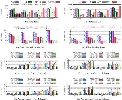
Figure 6. Tweaking the maxL parameter

Fig. 6(a) and 6(b) report the indexing time and size

for GR and the different maxL tried. For comparison,

we additionally include the corresponding values for SI methods. For all datasets, except PDBS, there is a difference of up to 3 orders of magnitude for both indexing time and

size and formaxLfrom 2 to 4, leading to times and sizes

even much smaller than the in use SI methods. For PDBS, the small number of labels and thus the small variation of enumerated paths leads to up to 1 order of magnitude

difference of the index size from maxL=2 to 4.

Fig. 6(c) and 6(d) present the pruning power of GR utilizing different feature sizes on all datasets. As it was expected, as we increase the size of the features, the CSS decreases and it affects accordingly the FPR. However, in all occasions the filtering power is better than that achieved by the SI methods. This is particularly evident in PPI, PCM and the Synthetic dataset. For these datasets and for all feature sizes, the CSS is very close to the ASS and we also get relatively small FPR values. PDBS follows the same trends but with less steep divergence from the SI methods because of the high ASS. This leads to the conclusion that we can

still achieve high speedups with smaller feature sizes. Fig. 6(e) - 6(h) report the achieved QLA and WLA

speedups by tweaking the maxLvalue of GR for the used

datasets for our hybrid FTV-SI solution when utilizing 1 and 4 threads and all query sizes. A notable thing here is that in some cases, with the sole exception of PDBS and PCM, the

achieved speedups with smaller maxL values outperform

the speedups with largermaxLvalues. We attribute this to

the fact that for smallermaxLvalues less time is required to

construct the index of the query and match it to the dataset’s index. Additionally, the fact that the candidate set sizes that are formed after GR’s filtering are close for the various

maxLvalues, constitutes to this end.

X. CONCLUSIONS

(11)

against that of SI methods. Having that in mind and knowing that the sub-iso testing can be very expensive as the graph DB grows large (in number or size of graphs), we set out to initially evaluate the performance of well known SI methods. Our experiments reveal no single winner across all datasets. We then evaluate the performance of a hybrid FTV-SI solution, which proves to be a better practice compared to the traditional SI methods over datasets consisting of a large number of graphs by bringing about significant speedups and rearrangements in algorithms’ relative performance with not yet a single winner. However gained benefits come at the extra costs of index space and time. Thus, we further analyzed this hybrid method in 2 dimensions: First, to reduce the index costs, we lowered the size of indexed features. Our results revealed that the filtering power of the FTV index is still much higher than that of SI methods and that high speedups can be achieved, even with smaller indexes, which are in turn even smaller than the SI ones. Second, as the time to perform index-based filtering is substantial, we studied the positive effects of doing this in parallel. Our results showed that expected speedups can be significantly boosted. We note that parallelizing this filtering step is a much easier task than parallelizing the actual SI method. Overall, this work surfaces new promising possibilities for expediting subgraph queries in graph DBs by experimentally revealing a blind spot in current thinking. We hope this will inspire new research targeting new FTV-style indexes and/or SI-style sub-iso algorithms for FTV-SI hybrids.

Acknowledgment.This work was co-funded by the

Eras-mus+ Programme of the European Union under the PRIMES project (no. 2016-1-UK01-KA201-024631). The contents of this publication are the sole responsibility of the authors and can in no way be taken to reflect the views of the National Agency and the Commission.

REFERENCES

[1] W.-S. Han, J. Lee, M.-D. Pham, and J. X. Yu, “iGraph: a framework for comparisons of disk-based graph indexing techniques,”PVLDB, vol. 3, no. 1-2, 2010.

[2] F. Katsarou, N. Ntarmos, and P. Triantafillou, “Performance and scalability of indexed subgraph query processing meth-ods,”PVLDB, vol. 8, no. 12, pp. 1566–1577, 2015. [3] J. Lee, W.-S. Han, R. Kasperovics, and J.-H. Lee, “An

in-depth comparison of subgraph isomorphism algorithms in graph databases,”PVLDB, vol. 6, no. 2, 2012.

[4] F. Katsarou, N. Ntarmos, and P. Triantafillou, “Subgraph Querying with Parallel Use of Query Rewritings and Alter-native Algorithms,” inProc. ACM EDBT, 2017.

[5] W.-S. Han, J. Lee, and J.-H. Lee, “Turboiso: towards ultrafast

and robust subgraph isomorphism search in large graph databases,” inProc. SIGMOD, 2013, pp. 337–348.

[6] Z. Sun, H. Wang, H. Wang, B. Shao, and J. Li, “Efficient subgraph matching on billion node graphs,”PVLDB, vol. 5, no. 9, pp. 788–799, 2012.

[7] V. Bonnici, A. Ferro, R. Giugno, A. Pulvirenti, and D. Shasha, “Enhancing graph database indexing by suffix tree structure,”

inProc. IAPR PRIB. Springer, 2010.

[8] J. Cheng, Y. Ke, W. Ng, and A. Lu, “FG-index: towards verification-free query processing on graph databases,” in

Proc. SIGMOD, 2007, pp. 857–872.

[9] R. Giugno, V. Bonnici, N. Bombieri, A. Pulvirenti, A. Ferro, and D. Shasha, “GRAPES: A software for parallel searching on biological graphs targeting multi-core architectures,”PloS One, vol. 8, no. 10, 2013.

[10] K. Klein, N. Kriege, and P. Mutzel, “CT-index: Fingerprint-based graph indexing combining cycles and trees,” in Proc. ICDE, 2011, pp. 1115–1126.

[11] H. Shang, Y. Zhang, X. Lin, and J. X. Yu, “Taming verifi-cation hardness: an efficient algorithm for testing subgraph isomorphism,”PVLDB, vol. 1, no. 1, pp. 364–375, 2008. [12] X. Yan, P. S. Yu, and J. Han, “Graph indexing: a frequent

structure-based approach,” inProc. SIGMOD, 2004. [13] D. Yuan and P. Mitra, “Lindex: a lattice-based index for graph

databases,”VLDBJ, vol. 22, no. 2, pp. 229–252, 2013. [14] P. Zhao, J. X. Yu, and P. S. Yu, “Graph indexing: tree + delta

>= graph,” inPVLDB, 2007, pp. 938–949.

[15] L. Zou, L. Chen, J. X. Yu, and Y. Lu, “A novel spectral coding in a large graph database,” inEDBT, 2008.

[16] F. Bi, L. Chang, X. Lin, L. Qin, and W. Zhang, “Efficient subgraph matching by postponing cartesian products,” in

Proc. SIGMOD, 2016.

[17] P. Zhao and J. Han, “On graph query optimization in large networks,”PVLDB, vol. 3, no. 1-2, pp. 340–351, 2010. [18] H. He and A. K. Singh, “Graphs-at-a-time: query language

and access methods for graph databases,” inProc. SIGMOD, 2008, pp. 405–418.

[19] S. Zhang, S. Li, and J. Yang, “GADDI: Distance Index Based Subgraph Matching in Biological Networks,” in Proc. ACM EDBT, 2009, pp. 192–203.

[20] X. Ren and J. Wang, “Exploiting vertex relationships in speeding up subgraph isomorphism over large graphs,”

PVLDB, vol. 8, no. 5, pp. 617–628, 2015.

[21] P. Peng, L. Zou, L. Chen, X. Lin, and D. Zhao, “Answering subgraph queries over massive disk resident graphs,”WWW, vol. 19, no. 3, pp. 417–448, 2016.

[22] L. Lai, L. Qin, X. Lin, and L. Chang, “Scalable subgraph enumeration in mapreduce,”PVLDB, vol. 8, no. 10, 2015. [23] L. Lai, L. Qin, X. Lin, Y. Zhang, L. Chang, and S. Yang,

“Scalable distributed subgraph enumeration,”PVLDB, vol. 10, no. 3, pp. 217–228, 2016.

[24] J. Wang, N. Ntarmos, and P. Triantafillou, “Indexing query graphs to speedup graph query processing,” in Proc. ACM EDBT, 2016, pp. 41–52.

[25] ——, “GraphCache: A Caching System for Graph Queries,”

in Proc. ACM EDBT, 2017.

[26] M. Zhou, J. Yu, Y. Liu, Q. Dai, and L. Guo, “PatternTreeISO:

A Pattern Graph Correlation Framework for Accelerating Subgraph Isomorphism over Massive Graphs,” in Proc. CIKM, 2016.

[27] S. Zhang, J. Yang, and W. Jin, “SAPPER: subgraph indexing and approximate matching in large graphs,”PVLDB, vol. 3, no. 1-2, pp. 1185–1194, 2010.

[28] W. Lin, X. Xiao, J. Cheng, and S. S. Bhowmick, “Efficient algorithms for generalized subgraph query processing,” in

Proc. CIKM, 2012, pp. 325–334.

[29] K. Semertzidis and E. Pitoura, “Durable graph pattern queries on historical graphs,” inProc. ICDE, 2016.

[30] L. P. Cordella, P. Foggia, C. Sansone, and M. Vento, “A (sub) graph isomorphism algorithm for matching large graphs,”