Essays on Bayesian persuasion

(1)

warwick.ac.uk/lib-publications

A Thesis Submitted for the Degree of PhD at the University of Warwick

Permanent WRAP URL:

http://wrap.warwick.ac.uk/104204

Copyright and reuse:

This thesis is made available online and is protected by original copyright. Please scroll down to view the document itself.

Please refer to the repository record for this item for information to help you to cite it. Our policy information is available from the repository home page.

(2)

Essays On Bayesian Persuasion

Davit Khantadze

A thesis presented for the degree o f Doctor of

Philosophy

Department of Economics

University of Warwik

(3)

Acknowledgments

I want to thank my advisors Ilan Kremer and Motty Perry for their guidance. I am especially grateful to Ilan Kremer for encouragement and insightful discussions.

I also would like to thank Kirill Pogorelskiy who read my paper. I am grateful to various faculty members at the economics depart-ment at Warwick for stimulating conversations.

I would like to thank Philipp Külpmann for being an excellent co-author.

Financial support from the economics department at Warwick and ESRC studentship made my stay at Warwick possible. I appreciate this.

(6)

Declaration

I declare that all the following work was carried out by me. Except the following:

(7)

Abstract

Chapter 1 reviews the literature about the bayesian persuasion. It first describes two main approaches to bayesian persuasion: concavifica-tion approach and informaconcavifica-tion design approach. Next I consider some extensions to the basic model of bayesian persuasion, like competi-tion between different senders, privately informed receiver and dy-namic bayesian persuasion. Some other contributions reviewed in-clude costly bayesian persuasion and bayesian persuasion when re-ceiver’s optimal action is only a function of an expected state.

Chapter 2 deals with two-dimensional bayesian persuasion. In this chapter I investigate a model when the receiver has to make two de-cisions. I am interested in optimal signal structures for the sender. I describe the upper bound of sender’s payoff in terms of his pay-off when only marginal distributions of two dimensions are known. Completely characterise optimal simultaneous and sequential signal structures, when each dimension has binary states. This approach ex-tends concavification approach to bigger state space, than explored in previous contributions to bayesian persuasion. Finally I characterise optimal sequential signal structure when there are three states for each dimension.

(8)

Chapter 1 Literature review

1.1 Introduction

Economists aim to solve optimisation problems; the latter can take dif-ferent forms. In the current paper we want to discuss a class of pa-pers that broadly deal with bayesian pa-persuasion, i.e. how one party, the sender, can provide information optimally to the other party, the receiver. Optimality means maximising sender’s payoff. The inten-tion of the literature on bayesian persuasion is to understand situa-tions, where one party has to make a decision based on the informa-tion provided by the other party. Examples might be following: seller can provide some information to the buyer about the product quality; the prosecutor undertakes investigation about the crime and provides this information to the judge; politician provides information about the quality of the project to the public. The question becomes inter-esting if there is some conflict of interest between the sender and the receiver. The seller might want to sell the product independent of it’s quality, whereas the buyer wants to buy the product only if the qual-ity is good. The prosecutor might want to send the defendant into the prison independent if the latter is guilty or not, whereas the judge wants to declare guilty only if the defendant is indeed guilty.

(9)

to bayesian persuasion; first approach, made popular by Kamenica and Gentzkow [2011], uses the concavification argument, as devel-oped by Aumann and Maschler [1995]; second approach uses the con-cept of bayesian equilibrium and extends it to the case where the me-diator has informational advantage relative to the players of the game. This approach was pioneered in a series of papers by Bergemann and Morris [2016a,b]. Next, in section 1.3 we discuss the case when multi-ple senders try to persuade a single receiver. Section 1.4 reviews liter-ature about informed receiver, i.e. when receiver has some additional information. In section 1.5 we review two papers that deal with dy-namic setting. Last section briefly reviews some other approaches to bayesian persuasion.

1.2 Different approaches to bayesian

persua-sion

In this section we discuss how economists think about acquiring infor-mation by sender, when he does not have commitment problems. First we explore the concavification approach.

1.2.1 Choosing optimal posterior distributions -

Con-cavification approach

Let’s consider following problem: receiver has to make a decision

-a. Sender has preferences over receiver’s actions. Receiver’s optimal

action is a function of his beliefs -ba(µ). For example judge’s decision is

a function of his belief about defendant being guilty or innocent. Say

sender can choose, given some common priorµ0, receiver’s posteriors.

What is the optimal way for him to do this? This question is dealt by Kamenica and Gentzkow [2011] and we intend to reproduce here some of their main arguments.

Receiver’s utility is a function of his action and of the state of the

(10)

the world. The knowledge about state of the world is given by

com-mon prior distribution µ0 ∈ 4(Ω). Sender can influence receiver’s

beliefs by choosing a signal. Signal is a mapping π : Ω → 4(S).

It means that sender can choose conditional distributions given state,

π(.|ω). Probability distribution is over some signal realisation space S

and si is some element in S. While it might not be immediate how to

address the problem of choosing optimal information structure, con-cavification argument says that there exists a simple solution to this problem if one is able to draw the graph of sender’s value function as a function of receiver’s beliefs. Before further exploring this question let’s consider following example, that was formulated by Bergemann and Morris [2016a] and is equivalent to the example by Kamenica and Gentzkow [2011].

A depositor has to decide to stay with the bank (s) or not (r). State

of the world is good (G) or bad (B) and bank is solvent if ω = Gand

insolvent ifω = B. Depositor and regulator have common prior and

assign equal probability to both states. Depositor’s utility function is the following:

u(s,G) = y u(s,B) =−1

u(r,G) = 0 u(r,B) =0 (1.1)

We assume thaty ∈ (0, 1)in general. For this exampley=0.5.

Regulator prefers depositor to stay with the bank, independent of

the state of the world. Regulator’s utility if depositor chooses(s) is 1

and 0 if depositor chooses(r). While it might not be immediate what

is the optimal signal for the regulator, analysing regulator’s problem geometrically, makes solution straightforward.

Before doing this, first we want to summarise the concavification approach, as formulated by Kamenica and Gentzkow [2011].

Let’s state one observation, that will turn out helpful in our search for optimal signal structure.

(11)

µ(ω) = µ(ω|s1)p(s1) +...+µ(ω|sn)p(sn) (1.2)

Equation 1.2 says that for any signal expected posterior must equal to prior. In turns out that this is the only constraint that a distribution of posterior beliefs has to satisfy.

Following observation is important for the concavification approach: instead of thinking about a particular signal, one can think about the distribution of posterior beliefs, that satisfy equation 1.2. We repro-duce Kamenica and Gentzkow [2011]’s result here.

Proposition 1. Following statements are equivalent:

i There exists a signal that gives sender some expected payoff v∗;

ii There exists a distribution of posteriors, whose expectation equals to prior and sender’s expected payoff equals v∗.

Let’s denote sender’s value function by υ(µ) and it’s convex hull

byco(υ). Now we want to introduce the concept of concavification of

the function. Given priorµ, sender’s maximum feasible payoff can be

described in the following way:

V(µ) ≡ sup{x2|(µ,x2)∈ co(ν)} (1.3)

V(µ) is the smallest concave function everywhere weakly greater

thanυ(µ) and Aumann and Maschler [1995] refer toV(µ)as the

con-cavification ofυ(µ).

Now we can summarise concavification approach to finding sender’s optimal signal structure:

1 : Draw sender’s value function as a function of posterior beliefs

-υ(µ)

2 : Draw the concave closure of υ−V(µ)

3 : Find distribution of posteriorsµs−(τ), s.t. Eτυ =V(µ)

(12)

[image:12.595.166.430.120.371.2]

Figure 1.1: Concavification of a function - an example; copied from Kamenica and Gentzkow [2011]

Kamenica and Gentzkow [2011] show that step 4 is always possi-ble.

We will use this approach to find regulator’s optimal signal.

First we want to construct regulator’s value function as a

func-tion of depositor’s beliefs. If µ(ω = G) < 2₃ then ˆa(µ) = r and if

µ(ω = G) ≥ 2₃, then ˆa(µ) = s. Thus regulator’s value function,

with-out signals, is the following:

0 if µ(ω =G) < 2

3 (1.4)

1 if µ(ω =G) ≥ 2

3 (1.5)

Now, by using equation 1.2 we are able to describe all possible ex-pected payoffs regulator can achieve by choosing some signal struc-ture. Regulator’s feasible expected payoffs can be described in the

(13)

[image:13.595.166.432.113.290.2]

Figure 1.2: Concavification of regulator’s value function

1.2.

Concavification of regulator’s value function is the following:

V(µ) =min{3

2µ, 1} (1.6)

Optimisation implies that regulator would choose highest avail-able expected payoff. One can see that this payoff is given by the

fol-lowing formula: λ2₃ + (1−λ)0 = 1₂, where λ is the probability that

posterior equals 2₃. So, regulator can choose a signal structure that

in-duces following distribution of posterior beliefs:

µ= 2

3 with probability

3

4 (1.7)

µ =0 with probability 1

4 (1.8)

What is the signal structure that gives this distribution of poste-riors? Note that bayes rule, together with equation 1.7 implies that

π(ss|ω = G) = 1. Therefore following signal structure induces

(14)

π(ss|ω =G) = 1 π(ss|ω =G) = 1

2

p(sr|ω =G) = 0 π(sr|ω =B) = 1

2

(1.9)

Now we have accomplished the following: we described a rela-tively simple procedure how to find a joint distribution of signal reali-sations and states that is most favourable for the regulator.

ω =G ω =B

sr 0.50 0.25 ss 0.00 0.25

The goal of the exercise was to show that when one can graph the value function of the sender as a function of beliefs, then one can find optimal signal structure by first finding optimal distribution of poste-rior beliefs.

Now we describe information design approach to bayesian persua-sion, as suggested by Bergemann and Morris [2016a,b].

1.2.2 Information design approach to bayesian

persua-sion

Bergemann and Morris [2016a,b] develop an information design ap-proach, that uses the concept of mediator, which gives recommen-dations possibly to multiple receivers. They show that if there is a single receiver, then their approach to information design reduces to "bayesian persuasion". As we will see, the information design ap-proach makes it relatively easy to model the private information of the receiver, i.e. when the receiver also observes additional, possibly pub-lic, informative signal about the state of the world. Before discussing the case of the receiver with additional information, we will discuss the above example by using the concepts as suggested by Bergemann and Morris [2016a,b].

(15)

given state; therefore we say that mediator has an information

advan-tage. Let’s denote byρθ regulator’s recommendation for the depositor

to run, when the state is θ ∈ {B,G}. Now, regulator’s

recommenda-tion has to satisfy obedience constraint, i.e. it has to be optimal for the depositor to follow the recommendation. Therefore, the depositor will have an incentive to stay, if

(1/2)(1−ρG)(1/2)−(1/2)(1−ρB) ≥0, (1.10)

and an incentive to run if

0≥(1/2)ρG(1/2) + (1/2)ρB(−1). (1.11)

We note that obedience constraint for staying 1.10 implies obedi-ence constraint for run 1.11.

Therefore, we can write 1.10 in the following form:

ρB ≥1− 1

2+

1

2ρG (1.12)

Say regulator’s goal is to minimise the probability of depositor

run-ning, then we see from inequality 1.12 thatρG = 0 andρB = 1₂. Note

that this recommendation rule will make the depositor stay with

prob-ability 3₄. Note also that recommendation rule and signal structure as

given in the expression 1.9 coincide.

After having described general approaches to bayesian persuasion, now we will discuss contributions that extend bayesian persuasion as described above in several dimensions. First we will discuss the case of several senders, i.e. when there is a competition between senders.

1.3 Competition in Persuasion

Our discussion of competition in persuasion is based on the following contributions by Gentzkow and Kamenica [2016a, 2017a].

(16)

that competition among senders will increase the amount of informa-tion revealed. To begin with, Gentzkow and Kamenica [2016a] con-struct an example where competition among firms reduces the amount of information revealed. It turns out that there is a simple characteri-sation of information structures that guarantees that competition does not decrease the amount of information. Competition can not decrease the amount of information revealed if and only if following is true: every player can induce any feasible distribution of posteriors that is more informative than posteriors induced by all other senders. One distribution of beliefs is more informative than other, if it is a mean preserving spread of the other. Gentzkow and Kamenica [2016a] call this condition Blackwell-connected. So, if information structure is not Blackwell-connected one can construct an example when competition can decrease the amount of information revealed.

One also would like to know what is the equilibrium outcome when there is competition among senders. To be able to describe equilibrium outcomes one has to assume that all senders have access to the same set of signals. Call a distribution of beliefs unimprovable for sender i, if for any other feasible distribution of beliefs sender i would not be better off. Then, Gentzkow and Kamenica [2016a] are able to prove following result:

Proposition 2. Say information environment is Blackwell-connected and each sender has access to the same set of signals. Then a feasible outcome is an equilibrium outcome if and only if it is unimprovable for each sender.

One can see that if an outcome is not unimprovable, then Blackwell-connected means that there exists a sender i that can increase his pay-off by inducing a more informative distribution of beliefs, that will in-crease his payoff. From this characterisation of the set of equilibrium outcomes it follows that one can easily find this set: one has to find the intersection of unimprovable outcomes. Unimprovable outcome can be described in the following way: the support of the distribution of

posteriorsµis such thatv(µ) =V(µ), wherev(µ)is sender’s expected

utility without signal and V(µ) is concavification of sender’s value

(17)

optimality implies this condition. But with many senders, Gentzkow and Kamenica [2016a, 2017a] show that this condition should be satis-fied for all senders.

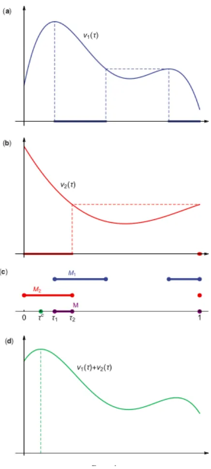
We will illustrate this by the following example: Graph (a)depicts

value function of sender 1 and graph(b)of sender 2. Solid line

inter-vals indicate unimprovable beliefs for each sender. The set of equilib-rium outcomes is the intersection of these sets and in this example is the following: [τ1,τ2]∪ {1}.

Horizontal axis in the graph depicts the share of facts revealed, so 1 means that all facts are revealed; therefore moving to the right of the horizontal axis means revealing more information.

Graph (d) depicts the collusive outcome, i.e. revealed facts that

maximise senders 1 and 2 overall payoffs. As one can see all equilib-rium outcomes reveal more facts than collusive outcome. This is in ac-cordance with the claim that if information environment is Blackwell-connected then collusive outcome can not reveal more information.

One can also see that fully informative outcome is an equilibrium. This follows from proposition 2. So, if all senders choose from the same set of signals and information environment is Blackwell-connected, then most informative feasible outcome is always an equilibrium.

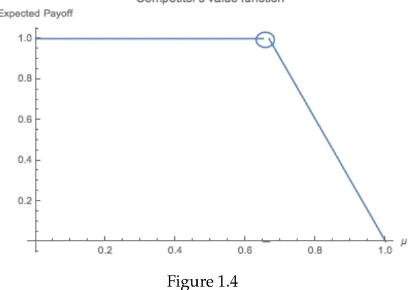
We could apply these ideas to our example about regulator and depositor. Say there also exists another, competing bank that prefers depositor to run than to stay. So it gets payoff 1 if the depositor runs and 0 if it stays. Let’s call it competitor. It can also produce signals for the depositor. Assume that depositor stays if his posterior of bank

being good is at least 2₃. Then concavification of competitor’s value

function is given in figure 1.4.

So, when regulator chooses his optimal signal, then competitor could reveal information about the bank and increase it’s payoff. The only equilibrium outcome of this game is fully informative signals. Note that when fully informative signals are produced, then for any

posterior beliefµ, following is true for both regulator and competitor:

(18)

[image:18.595.176.394.156.639.2]

(19)

[image:19.595.150.453.120.331.2]

Figure 1.4

This example shows that sender can be worse off from competition, because receiver gets more information. Here receiver’s additional in-formation is an outcome of strategic interaction between competing senders. Next we want to review literature that explores following question: receiver gets informative public signal about the state of the world.

1.4 Informed receiver(s)

Bergemann and Morris [2016a] divide information design in two steps: first, describe the set of feasible outcomes in general and second de-scribe what outcomes will be chosen from an interested party and what is the information structure that leads to these outcomes.

These approach was already used in section(1.2.2)while discussing

information design approach to bayesian persuasion. Now we will il-lustrate it for the case when the depositor observes informative public signal about the state of the world.

(20)

ω =G ω =B

g q₂ 1−₂q

b 1−₂q ₂q

q> 1₂.

The set of feasible outcomes will also be determined by the follow-ing: the regulator observes depositor’s public signal or not. First let’s consider the case when the public signal, i.e. depositor’s additional information, is observed by the regulator. Therefore, regulator’s rec-ommendation will be a function of the state and the signal observed.

Now for a recommendation to stay to satisfy obedience constraint, i.e. for depositor to have an incentive to follow the recommendation, it should take into account depositor’s conditional belief about the state of the world that he forms after observing the public signal. So, when the depositor observes good signal, then he will follow the recommen-dation to stay, if

q(1−ρGg)(1/2)−(1−q)(1−ρBg) ≥0 (1.13)

Similarly, depositor will follow the recommendation to run after he observed the good signal, if:

0≥qρGg(1/2) + (1−q)ρBg(−1). (1.14)

Similar conditions have to be satisfied if the public signal is bad. In expectation, for a recommendation to be followed, following condition should be satisfied, that we give in a form of proposition:

Proposition 3. The probabilities ρB,ρG form an equilibrium outcome for some information structure if

ρB ≥maxq(1+1

2), 1 −

1

2+

1

2ρG. (1.15)

This describes the set of all possible recommendation rules that

sat-isfy obedience constraint. As the precision of the public signal(q)

in-creases, ρG becomes 0 and ρB becomes 1, so the only feasible

(21)

informed about the state of the world from observing the public sig-nal, there is not much the regulator can do by providing additional information.

Bergemann and Morris [2016a] show that the set of feasible out-comes shrinks when the depositor gets additional information and this information is also observed by the regulator. This set shrinks even more if depositor’s additional information is not observed by the reg-ulator and he has to elicit if from the depositor.

Bergemann and Morris [2016b] extend the result that receiver’s ad-ditional information reduces the set of feasible outcomes to many play-ers case. They identify the condition of "more informative" in the sense of Blackwell in the case of many players, for which the result extends to the many player setting.

Kolotilin et al. [forthcoming] consider following question: receiver has private information about his preferences; sender can commit to information disclosure about the state. Sender’s and receiver’s utili-ties are linear function of the state and receiver’s type. Sender, before choosing a signal structure could ask the receiver his type and the sig-nal could be a function of the receiver’s report. Or sender could choose a signal structure independent of receiver’s report. Kolotilin et al. [forthcoming] show that in their setting there is no loss of generality in considering only signal structures. Therefore sender can ignore more complex persuasion mechanisms and produce signal without asking the receiver to report his type.

Now we will discuss some papers that deal with bayesian persua-sion in the dynamic context.

1.5 Dynamic bayesian persuasion

1.5.1 Ely: Beeps

(22)

principal changes agent’s current belief and also shapes the path of it’s further evolution. Ely [2017] extends the approach to information pro-vision as formulated by Aumann and Maschler [1995] and Kamenica and Gentzkow [2011] to the dynamic setting. In particular he extends the insight that it is without loss of generality to analyse distribution of posterior beliefs, s.t. expectation equals prior, to the dynamic setting and one can use geometric approach to find optimum distribution of posteriors and optimal signal that induces it.

Ely [2017] considers following motivating example. An agent has to work, but is distracted by checking emails. The IT-department (prin-cipal) considers how to filter information so that the agent checks the email as late as possible. Principal could use the email notification soft-ware that beeps when the email arrives. If the softsoft-ware is switched on, then the worker stops working when he hears the beep. E-mail arrival

is modelled as a poisson process. The e-mail arrival rate isλ. So, if the

software is switched on, then expected arrival time of the e-mail is 1_λ.

Principal could decide to switch-off the software. Assume that the

agent has a threshold belief p∗, s.t. when his belief is at least as big

as p∗, then he checks the e-mail. When the beep is turned off, then

agent’s belief that an email has arrived is 1−e−λt_{and therefore agent’s}

working time is the following:

t∗ =−log(1−p

∗₎

λ (1.16)

By comparing equation (1.16) with _λ1 one can see that for high p∗

agent will work longer if beep is turned off. If p∗ is low enough then

agent works longer when beep is turned on.

(23)

mechanism, that turns out to be also optimal: beep with a delay. If

e-mail arrives at date t, the agent hears beep at date t+t∗. Expected

time of work, as induced by this mechanism, ist∗+_λ1.

Note that the suggested mechanism accomplishes the following:

when principal’s and agent’s interests are aligned, i.e. t≤t∗, principal

does nothing. Whent > t∗, i.e. agent’s belief, without information, is

such that he would check the e-mail, then principal filters information

such that agent’s belief is either p∗ or 1. Note the resemblance to the

depositor case, where the depositor learns the true state only if the state is bad. Similarly in the current example the agent learns that

email has arrived only ift >t∗, i.e. he would check the e-mail if there

was no additional information provided by the principal.

How does the suggested mechanism accomplish this? Because the

agent hears the beep with delayt∗, it means that he does not hear beep

for the period oft∗. Say t > t∗ and the agent has not heard the beep.

Then the agent knows that e-mail has not arrivedt∗periods before and

his belief isp∗.

Before giving the proof that this is principal’s optimal mechanism, we briefly describe how to extend the insight from the static bayesian persuasion that it is without loss of generality to consider distribu-tion of posterior beliefs, whose expectadistribu-tion equals prior. In the dy-namic context Ely [2017] shows that it is without loss of generality to directly choose a stochastic process for the agent’s beliefs, given that this process satisfies two properties: expected posterior equals prior and agent’s belief evolves according to the state transition probability. Ely [2017] first guesses principal’s optimal strategy, which is de-layed beep. The value function for this strategy, for agent’s current

beliefµt being smaller than the critical value, i.e. µ ≤ p∗, is given by

the following equation:

V(µ) = 1

r

(1−e−rτ(µ)_{) +}_e−rτ(µ) r

r+λ

(1.17)

(24)

There-Figure 1.5: Value function for the t∗−delayed beep - copied from Ely [2017]

fore, the guessed value function is given by figure 1.5

Proving optimality consists in showing that the suggested strategy is unimprovable. By taking into account that feasible policies induce distribution of posterior beliefs whose expectation equals prior belief, one has to consider deviations that satisfy this condition. But then, given this constraint, one can describe the optimal value as a concavi-fication of the value function. Ely [2017] verifies that principal’s opti-mal payoff from one-shot deviation coincides with the suggested value function arising from the strategy of delayed beep.

Optimal payoff can be formulated in the following form:

rV =cav

u+V0· dv

dv

[image:24.595.144.518.125.407.2]

(25)

[image:25.595.149.525.121.428.2]

Figure 1.6: Concavification - copied from Ely [2017]

where, cav denotes concavification of the expression in the bracket.

Graph of the expression in the bracket of equation(1.18)is the

follow-ing:

Concavification argument also explains why delayed beep is an

op-timal strategy. The value function without signal is concave forµ ≤ p∗,

therefore it is optimal for the principal to not reveal any information

and this is accomplished when beep is delayed by t∗. When agent’s

belief becomes bigger than p∗, then concavification is strictly higher

than the value function without signal. In this case the induced

poste-rior beliefs are either p∗or 1 and this is accomplished by the suggested

strategy.

(26)

1.5.2 Hörner and Skrzypacz: Selling Information

Hörner and Skrzypacz [2016] analyse following situation: firm (it) con-siders to hire an agent (she) to implement a project. Agent can be of

good (1) or bad (0) type. It pays off for the firm to implement the

project only if the agent is of good type. Agent knows her type. Be-fore the firm makes hiring decision, agent and firm can communicate in several stages; during each communication stage transfers can be made and agent can reveal information about her type by choosing a test. Hörner and Skrzypacz [2016] are interested in the following question: how can a competent agent persuade the firm to hire her and still be rewarded for the competence? Motivation for this ques-tion is to understand incentives of the agent for acquiring the compe-tence. Formally, authors are interested in finding best possible equilib-rium outcome for the competent agent. They show that agent increases her payoff by revealing information gradually. Before reproducing the argument for gradualism, we briefly describe the set-up, that should help the exposition.

The firm decides to hire the agent and implement the project, only if his belief that agent is competent is above some threshold, denoted

by p∗. Firm’s belief determines his outside option, that we denote by

w(p). If p > p∗, then firm’s outside option is positive, otherwise it is

0. We assume that p0 < p∗, i.e. firm’s prior belief is smaller than the

threshold. Firm’s payoff from hiring a competent agent is 1; therefore from firm’s perspective, when he beliefs that agent is competent with

probabilityp, expected overall surplus isp.

Prior of hiring decision agent and firm communicate forKstages.

The agent can choose the difficulty of the test in each

communica-tion stage. Denote test’s difficulty bym ∈ [0, 1]. m is the probability

with which the test is passed by the incompetent agent. Competent agent passes the test with probability 1.

The choice of test-technology leads to a distribution of posteriors

that equals to prior. So, if m is such that in case the test is passed,

posterior becomes p0, then one knows also distribution of posteriors,

(27)

Firm’s expected gain, when the agent chooses test-technology, is given by the following equation:

EF[w(p0)]−w(p) (1.19)

where EF[ ]is firm’s expectation operator.

Hörner and Skrzypacz [2016] consider an equilibrium, where in each communication stage the firm pays it’s entire expected gain from the additional information to the agent.

Now we are ready to show why gradual information provision benefits the agent. Say there is 1 round of communication.

By the argument as formulated in proposition(1), Hörner and

Skrzy-pacz [2016] look at the distribution of posterior beliefs. Say agent

chooses some test that, if it is passed, leads to a posterior beliefp1 ≥ p0.

From the law of total probability then follows that posterior becomes

p1 with probability pp01. By using this information, equation (1.19)

be-comes

p0 p1

w(p1)−w(p0) (1.20)

Because we are considering the case when p0< p∗, thereforew(p0) =

0, i.e. firm does not implement the project. One can show that w(p1)

p1 is

increasing inp1, therefore one can see that with one stage

communica-tion maximum the competent agent can achieve is to choose a perfectly

informative test, so that p1 = 1. The firm would be willing to pay p0

for such a test, i.e. with one stage communication competent agent can get ex-ante expected surplus.

But the agent can increase her payoff by offering two tests. First

test is chosen such thatp1= p∗. Remember thatw(p∗) = 0. Therefore

the firm’s willingness to pay for this test is 0. Given new posterior p∗,

then by repeating the argument of one stage communication, second

(28)

[image:28.595.164.427.127.352.2]

Figure 1.7: Revealing information in two steps - copied from Hörner and Skrzypacz [2016]

Figure 1.7 visualises this argument. Diagonal denotes expected

surplus. w(p)0s curve is below diagonal line and equals 0 for p< p∗.

Can the agent do better than this by offering more tests? Following example shows that the answer to this question is positive.

Consider now the case when the competent agent offers three tests

that lead to the following posteriors: p∗, p0and 1.

Figure 1.8 illustrates agent’s payoff from offering three tests. Agent’s overall payoff one gets by summing two red vertical lines. One can see that by offering three tests agent can get higher payoff than by offer-ing only two tests. Agent’s payoff when only two tests are offered is given by summing the left red line segment and the dashed line seg-ment above it. But as one sees the right red line segseg-ment is bigger than the dashed line segment.

Hörner and Skrzypacz [2016] show that whenp0 < p∗, then agent’s

payoff is maximised by first giving information for free and making

posterior equal top∗and then dividing the interval[p∗, 1]into smaller

(29)

[image:29.595.169.430.118.333.2]

Figure 1.8: Revealing information in three steps - copied from Hörner and Skrzypacz [2016]

Now we briefly survey some other contributions to bayesian per-suasion.

1.6 Further contributions to bayesian

persua-sion

Concavification approach requires that sender’s value function can be expressed as a function of receiver’s beliefs. Gentzkow and Kamenica [2014] consider the case when producing signal is costly. They charac-terise the class of cost functions which is compatible with concavifica-tion approach. Thus, Gentzkow and Kamenica [2014] extend concavi-fication approach to the case when signals are costly.

(30)

Gentzkow and Kamenica [2016b] considers the setting where re-ceiver’s optimal action is a function of expected state and sender’s payoff depends only on receiver’s action. Authors characterise the set of distribution of posterior means that can be achieved by some signal.

1.7 Multidimensional persuasion

(31)

Chapter 2 Two-dimensional bayesian

persuasion

2.1 Introduction

A software company (sender) wants to sell two products (A and B) to the customer (receiver). Sender has to decide how to provide infor-mation to maximise the likelihood of receiver buying two products. Sender can choose precision of the information about the products. What is the optimal way to accomplish this when the information about one product also contains indirectly information about the other product?

For illustration, we consider the following example: each product

can be good(1)or bad(0). Receiver gets utility 1 if he buys the good

product or does not buy the bad product and 0 otherwise. Receiver’s utility is additively separably in two products. So, if receiver buys both products and each is good, then his utility is 2. Sender’s utility is also additively separable in two products and his utility is 1 if receiver buys a product and 0 otherwise. Sender and receiver share common prior belief about the quality of two products, that is given in figure 2.1.

(32)

B =1 B=0 A=1 0.30 0.15 A=0 0.05 0.50

Figure 2.1: Motivating Example

precision, i.e. test could inform perfectly about the product(s) or not inform at all.

If Aand Bwere independent, then solution to the problem is well

known. One has two separate persuasion problems and optimal sig-nal for each product can easily be found by using concavification ar-gument as developed by Aumann and Maschler [1995] and further explored by Kamenica and Gentzkow [2011]. It is well known that concavification approach makes it easy to find optimal signal when the state space is relatively small and it is not straightforward how to use this approach when state space becomes large. This is so, because it relies on geometric argument and requires visualisation to find an optimal signal. This is pointed out for example by Gentzkow and Ka-menica [2016b], when they mention the following: "... the value func-tion and it’s concavificafunc-tion can be visualised easily only when there are two or three states of the world." Therefore, for a state space bigger than this, it is not immediate how to use concavification of the value function in order to find optimal signal. Thus note that for a simplest possible, non-trivial two-dimensional bayesian persuasion problem it is not immediate how to use concavification approach to find an opti-mal signal of the sender.

If the sender decides to split the persuasion problem into two parts and first inform about one product and then about the other, he also has to take into consideration the fact that the signal about one product also informs about the other product.

In the current example if the sender decides to inform first only about product B and then, given new posterior, inform about product A, one can show that sender’s payoff would be smaller than if only

marginal distributions of A and B were known. But if he chooses to

(33)

gives sender the same payoff as what he would get if only marginal distributions were known. But can the sender do better than this? And does there always exist a signal that informs separately about two products that achieves for the sender the same payoff as when only marginal distributions are known?

We show for the preference specification of our model that the ad-ditional information in the form of joint distribution acts as an addi-tional constraint for the sender and for arbitrary number of states for each dimension, sender can never achieve a higher payoff than what he would get if only marginal distributions were known.

From this follows for the current example that there exists a simple procedure for the sender to maximise his payoff: first inform about

product Aand then inform about productB.

Why does the signal that first informs about B and then about A

fail to achieve the upper bound? Because it reveals too much

infor-mation about product A. We describe for arbitrary number of states

and for the given preferences of the current model, the necessary and sufficient condition for signals that inform about products separately to achieve the upper bound. This condition states that the support of the distribution of posteriors of one product, as induced by the sig-nal of the other product, should belong to the interval, on which the concavification of sender’s value function for this product is linear.

Next we show that when there are two states for each dimension

and if A and B are positively correlated then there always exists a

signal that informs about products separately and achieves the upper bound of the payoff for the sender.

We also show by giving an example that there exist joint distribu-tions, for which there does not exist a signal that informs about two products separately and achieves the upper bound.

The problem of informing about products separately is that the sig-nal about one product might reveal too much information about the other product. Sender can solve this problem by constructing a more complicated signal that informs about both products simultaneously.

(34)

simultaneous signal that informs about both products simultaneously and achieves the upper bound for arbitrary joint distribution.

Next we analyse the case when there are three states for each di-mension. Finding a signal that informs about both dimensions simul-taneously now means to find a joint distribution of signal space and decision relevant space that has up to 81 states. Currently we do not have solution for this problem. We describe a procedure of how to split this problem into two parts and inform about products separately. In particular we clarify when does this procedure achieve the upper bound for the sender.

The paper is organised in the following way: in the next section we briefly review the literature about bayesian persuasion. Then we describe our model. In section 2.4 we derive some general results. Sec-tion 2.5 analyses the case when there are two states for each dimension. Then we analyse optimal sequential signals when there are 3 states for each dimension.

2.2 Related work

Kamenica and Gentzkow [2011] analyse optimal information provi-sion when the single receiver has to make a single deciprovi-sion. They give a characterisation of optimal signals in a general framework, by using the concavification argument as formulated by Aumann and Maschler [1995]. This approach can be summarised in the following way: choos-ing a signal that maximises sender’s payoff is equivalent to chooschoos-ing optimal distribution of posteriors that equals prior in expectation. This distribution of posteriors can be found by drawing value function of the sender as a function of beliefs. After one has found optimal distri-bution of posteriors, one can also find signal that gives this posterior distribution, by using Bayes rule.

(35)

at-tainable outcomes. In the current setting, when the sender chooses to produce information sequentially, receiver’s additional information is controlled by the sender and is endogenous in this sense, but still can constrain sender’s achievable outcomes.

2.3 The model

2.3.1 Payoffs

The receiver faces two decision problem, A and B, which sometimes

we will refer to as dimensions 1 and 2. For each dimension the receiver wants to match the states of the world, which are non negative

inte-gers. Receiver’s utility function is −(aA−ωA)2−(aB−ωB)2, where

ai,ωi ∈ {0, 1, ...,n},i∈ {A,B}and some givenn. aidenotes receiver’s

action andωi denotes the state of the world for dimensioni. We will

denote joint state by ωA,B = (ωA,ωB), where ωA,B ∈ {0, 1, ...,n}2.

Sender’s utility function is aA+aB. So, the receiver wants to match

the state for each dimension, whereas the sender prefers the receiver choosing as high a number as possible for each dimension.

2.3.2 Signal structures

Receiver and sender have common prior joint distribution ofAandB.

Sender can choose a signal structure, which means, choosing a fam-ily of conditional distributions. The choice of the signal structure is common knowledge.

The sender could decide to inform aboutAandBseparately, which

means first producing signal say for A and then forB. We call this a

sequential signal structure. Or the sender could decide to produce signal for both dimensions simultaneously, i.e. choose a simultaneous signal structure.

If the sender decides to inform about Aand Bseparately, then we

(36)

2.3.3 Sequential signal structure and order of moves

A sequential signal structure informs immediately only about one di-mension. For simplicity here we assume that the first signal is

pro-duced for A and the second signal for B. Signal can be viewed as a

probability distribution over recommendations, which in equilibrium will be followed by the receiver.

Here we describe a sequential signal structure when the first

sig-nal is produced for A. Sender chooses a family of conditional

dis-tribution functions π(.|ωAi), over recommendations sAi ∈ S, where

i ∈ {0, 1, ...,n}. S denotes the space of signal realisations. The choice

of signal for A is common knowledge. Receiver observes signal

real-isation sAi and updates his beliefs about A by bayes rule. sAi can be

interpreted as a recommendation for the receiver to chooseifor A. In

equilibrium this recommendation will be followed.

After observing signal for A, receiver updates his beliefs about A

and takes an action forAthat is optimal given his beliefs aboutA.

Because the common prior is joint distribution of AandB, ifAand

Bare not independent and if the signal is not uninformative, then the

signal for A will also contain some information about B. Thus, after

updating beliefs about A, receiver’s beliefs aboutBmight also change.

Given these new beliefs about B the sender chooses a signal forB,

which is again a family of conditional distributions over

recommen-dations forB. Receiver observes the choice of the signal for Band the

signal realisation. Then updates his beliefs aboutBand takes an

opti-mal action forB.

When discussing sequential signal structures, we will refer to the

signal, say of A, as optimal, if for the sender this would be an optimal

signal forAif only marginal distributions of AandBwere known.

(37)

2.3.4 Simultaneous signal structure and order of moves

Sender can decide to provide information simultaneously about both dimensions. This can be accomplished by making signal a family of conditional distributions on the joint state space and thus informing

about both dimensions simultaneously. Now an element (s) of the

space of signal realisation (S) can be regarded as a recommendation

about two actions. Simultaneous signal isπ(.|ωA,B),ωA,B ∈ {0, 1, ...,n} ×

{0, 1, ...,n}. Signal realisation iss(i,j), where,iand j∈ {, 0, ..,n}, which

can be interpreted in the following way: chooseifor dimensionAand

jfor dimensionB.

Simultaneous signal accomplishes the following: given signal

re-alisation s(.,.), receiver forms beliefs about the joint distribution of A

andB. Then, given new joint distribution, receiver calculates marginal

distributions ofAand Band makes decisions for both dimensions.

2.3.5 Optimal signals

We are interested in signals that maximise sender’s expected payoff. Following Bergemann and Morris [2016a] sometimes we will refer to obedience constraint that signal should satisfy. This means for

exam-ple that if signal realisation is s(i,j), it can be interpreted as a direct

recommendation to the receiver to chooseifor dimension Aand jfor

dimension B and the receiver should have an incentive to follow this

recommendation, i.e. it should be optimal for the receiver to choose

i and j. Also sometimes, for easy of exposition, we will present the

signal as a joint distribution of signal space and the decision relevant space.

2.4 General Observations

In the current section we want to relate two-dimensional bayesian per-suasion of the current model to the one-dimensional bayesian prob-lem. The latter is equivalent to the case when only marginal

(38)

we want to describe receiver’s optimal payoff in terms of his payoff

when only marginal distributions of AandBare known.

Preference specification of our model means that receiver’s

opti-mal decision about dimensioniis only a function of expected state for

i. This follows from the fact that receiver’s preferences are additively

separable across dimensions A and B. This means that additional

in-formation in the form of joint distribution of Aand B acts like an

ad-ditional constraint for the sender. We formalise this observation in the following proposition.

Proposition 1. For arbitrary n and arbitrary joint distribution of A and B upper bound of sender’s expected payoff is what the sender could get if only marginal distributions of A and B were known.

Proof. Say there exists a signal that gives sender higher payoff than what he would get if only marginal distributions were known. This

means that there exists a dimensioni for which sender’s payoff from

the signal is higher than his optimal payoff for iif only marginal

dis-tribution ofiwas known. But because receiver’s optimal action about

dimensioniis only a function ofi’s expected state, this is a

contradic-tion.

This argument can be illustrated by the following reasoning. Say

the receiver has to make a single decision about dimension i. Then

the additional information about some irrelevant state of the world, in

the current case in the form of joint distribution ofi and the decision

irrelevant state of the world, can be of no benefit for the sender. In the

current model state of the world for dimensionjis irrelevant when the

receiver makes a decision abouti.

After describing upper bound for sender’s payoff, now we want to describe a necessary and sufficient condition for a sequential signal structure to achieve this upper bound. This will turn out helpful when finding optimal sequential signal structures.

(39)

Note also that for these marginal distributions, if the common prior was joint distribution, such that A and B were independent, then op-timal sequential signal structure would give sender the same payoff as when only marginal distributions are known. But if the common

prior is a joint distribution of Aand B and they are not independent,

then the signal for one dimension in general will also contain an in-formation about the other dimension. Before formulating our main argument, we make following two observations.

First, we have to remember that sender’s value function, V, with

signals, is concave by construction. This is the popular concavifica-tion argument as developed by Aumann and Maschler [1995] and Ka-menica and Gentzkow [2011]. For exposition purposes we briefly re-peat this argument. We follow here Kamenica and Gentzkow [2011].

Denote sender’s value function byv(p). Denote convex hull ofv(p)

by co(v). Then, concave closure of v(p) is defined in the following way:

V(p)≡ {z|(p,z) ∈ co(v)} (2.1)

Kamenica and Gentzkow [2011] show that sender’s optimal payoff

for a prior p0isV(p0).

We formalise these observations in the following lemma:

Lemma 1. Sender’s maximum payoff for belief p is V(p). Sender’s value function with signals, V, is concave by construction.

Second observation is that the signal foriinduces a probability

dis-tribution of posteriors ofjthat equals to the prior marginal distribution

of j. This follows from the law of total probability. We formalise this

observation in the following lemma:

Lemma 2. Signal for i induces a distribution of j’s posteriors, whose expec-tation equals to j’s prior.

(40)

Proposition 2. For arbitrary n and arbitrary joint distribution of A and B, there exists a sequential signal structure that achieves an upper bound, if and only if following is true:

There exists a dimension i s.t. first producing an optimal signal for i induces a distribution of posteriors of j whose support belongs to an interval on which sender’s value function for j is linear.

Proof. Say there exists such ani. Then, first producing an optimal

sig-nal forigives following expected payoff forj:

p(si0)V(β(si0)) +...+p(sin)V(β(sin)) =V(p(si0)β(si0)+...+

p(sin)β(sin)) = V(β)

(2.2)

Where, for example p(si0)is a probability of observing signal

reali-sationsi0, which leads to the posterior distribution(β(si0))ofj. V(β(si0))

is sender’s payoff for dimension j, when he chooses an optimal signal

for j, when the prior belief is (β(si0)). βis the prior marginal

distribu-tion ofj.

First equality follows from our assumption that the value function

of j is linear on the interval to which the support of the distribution

of j’s posteriors belongs, as induced by the optimal signal of i. The

second equality follows from lemma 2.

Now say there does not exist such ani. If the signal for the

dimen-sioniis optimal, then we get the following expression:

p(si0)V(β(si0)) +...+p(sin)V(β(sin))<V(p(si0)β(si0)+...+

p(sin)β(sin)) = V(β)

(2.3)

Inequality follows from Jensen’s inequality and lemma 1, because

V is not linear on the support of the distribution of j’s posteriors as

induced by the signal fori. Equality follows again from lemma 2.

(41)

Figure 2.2

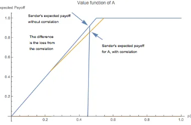
We want to show graphically how does the correlation between A

and Baffect sender’s payoff for A, when he chooses to provide

infor-mation sequentially and the first signal is produced for B. First we

briefly describe how to construct sender’s value function with signals.

One starts with sender’s utility function without signals. Sender’s

utility without signals is 0 if p(A = 1) < 1₂ and 1 if p(A = 1) ≥ 1₂

and is given in figure 2.2. Next we construct smallest concave function weakly bigger than sender’s utility function. So, if only marginal dis-tributions of A and B were known, then sender’s maximum payoff for

Ain the example from the introduction would be 0.90, because

small-est concave function everywhere weakly greater than sender’s value

function ismin{2p(A=1), 1}and is given in figure 2.3.

When the first optimal signal is produced for B, then the

poste-rior of Abecomes bigger than 0.5 with positive probability. Therefore,

the expected payoff for A, when the first signal is produced for B, is

smaller than if only marginal distribution ofAwas known.

In the next section we analyse optimal simultaneous and sequential

(42)

[image:42.595.119.500.113.363.2]

Figure 2.3: Concavification of value function; vertical line describes

the set of feasible payoffs for A, when p(A = 1) = 0.45 and Aand B

are independent.

2.5 Optimal simultaneous and sequential

sig-nal structures, when n=1

For the motivating example in the introduction, if the first signal is

pro-duced forAthen there exists a sequential signal structure that achieves

an upper bound. Following example 2.41shows that this is not true in

general, i.e. there exist joint distributions, for which there does not exist a sequential signal structure that achieves the upper bound.

To see this, note the following: if the first signal is produced for

dimensioni, thenp(i =0)is in the support of the distribution induced

by the optimal signal for i. But p(j = 1|i = 0) = 3₅. Therefore, it

follows from proposition 2 that there does not exist a sequential signal structure that achieves the upper bound.

This example shows that there exist joint distributions of A and

B, for which whatever the order of persuasion, if the first signal

(43)

B =1 B=0 A=1 1₉ 3₉

[image:43.595.241.356.112.174.2]

A=0 3₉ 2₉

Figure 2.4: Example, where no sequential signal can achieve an upper bound

duced is optimal, than the sequential information provision always reveals too much information to the receiver, than what is optimal for the sender.

So, the problem with a sequential signal structure is that it can re-veal too much information to the receiver. To hinder the receiver to learn about one dimension from the signal about the other dimension signal should inform about the joint state.

Now we derive an optimal simultaneous signal that conditions on the joint states and therefore induces a distribution of posterior beliefs about joint states.

2.5.1 Optimal simultaneous signal

To calculate optimal simultaneous signal when there are four states, we can not use concavification of the value function, since we will re-quire four dimensions to visualise sender’s value function as a func-tion of distribufunc-tion of beliefs. Instead, following Bergemann and Mor-ris [2016a] we will think about signal as a recommendation rule for the receiver, that should satisfy obedience constraint. For example, if

signal realisation iss(1,1), then receiver would choose 1 for A and B iff

p(i = 1|s(1,1)) ≥ 1₂, for i ∈ {A,B}. For ease of notation we will

rep-resent the signal as a joint distribution of decision relevant state space

and signal space, i.e. joint distribution of ωA,B and s(i,j). Let’s denote

joint distribution of AandBin the following way:

B

(44)

where, for example, p(1, 0) denotes probability of the following

event: A=1 andB=0.

We will also use the following notation. Consider states (1, 0)and

(0, 1): letα denote the state that is less likely among these states and

β the state that is more likely. For example if p(1, 0) > p(0, 1), then

α = (0, 1) andβ = (1, 0). Also, if p(1, 0) = p(0, 1), then sayα = (1, 0)

and β = (0, 1). Then expression p(β) would mean more likely event

among {(1, 0),(0, 1)}, if p(1, 0) 6= p(0, 1) and p(0, 1) otherwise. Also

we will use the above notation of states for recommendations, i.e. s(α)

ands(β).

Now we can proof the following result:

Proposition 3. A optimal simultaneous signal is given by the following joint distribution:

s/ω (1, 1) α β (0, 0)

s(1,1) p(1, 1) p(α) p(α) p(1, 1)

s(α) 0 0 0 0

s(β) 0 0 p(β)−p(α) p(β)−p(α)

s(0,0) 0 0 0 p(0, 0)−[p(1, 1) +p(β)−p(α)]

Proof. First, note that signal recommendations satisfy obedience con-straints. Second, note that the payoff from this signal is the same as

what would be if only marginal distributions ofAandBwere known,

as induced by the joint distribution. Then, it follows from the proposi-tion 1 that this signal is optimal.

The suggested optimal simultaneous signal is not unique. Note

that the signal does not make a recommendation ofα if p(α) < p(β),

i.e. p(sα) = 0; and if p(α) = p(β), then p(sα) = p(sβ). One can

(45)

of A and B are known. To put it simply, we know that when only marginal distributions are known, then the support of the distribution

of posteriors as induced by the optimal signal is 0 and 1₂. This is true

also for the suggested optimal simultaneous signal. What we are say-ing is that although the signal is not unique, this property remains true for other optimal simultaneous signals as considered here. It still re-mains to be shown formally that this claim is true in general, i.e. for all optimal simultaneous signals.

After deriving sender’s optimal simultaneous signal, we want to analyse optimal sequential signal structures.

2.5.2 Sequential signal structure

Our goal is to find optimal sequential signal structures, whenn=1.

As we showed above, sender’s value function with signals for

di-mensioniis the following:

V(p(1)) =min{2p(1), 1} (2.4)

From equation (2.4)follows that sender’s value function with

sig-nals is linear on the interval[0, 0.5]. Therefore if the first signal is

pro-duced for A then for a sequential signal structure to achieve the same payoff as when only marginal distributions are known, it has to be the

case that support of the distribution of B’s posteriors, as induced by

the optimal signal for A, has to be in the interval[0, 0.5]. This follows

from proposition 2.

Corollary 1. There exists a sequential signal structure that achieves the same expected payoff for the sender as what he optimally can get if only marginal distributions were known, if and only if following is true: there exists a pair (i,j) s.t. first producing an optimal signal for i induces a distribution of j’s posteriors with support[0, 0.5].

(46)

which no sequential signal can achieve an upper bound. One

differ-ence between these examples is that in the first example A and B are

positively correlated, whereas in the second case they are negatively correlated.

Now we want to characterise joint distributions in terms of corre-lation that allow sequential signal that achieves an upper bound.

Signal for i directly informs only abouti. Thus, optimal signal for

iinduces two posteriors of j, one for si1and another forsi0. It follows

from the concavification argument that optimal signal fori induces a

distribution of posterior beliefs ofi, that has following support: p(i =

1|si1) = 12 and p(i =1|si0) = 0. Now we are interested in the support

of j0s posterior beliefs, as induced by the optimal signal for i. This

distribution has following support, expressed in terms of conditional probabilities:

p(j=1|si1) = 1

2[p(j =1|i =1) +p(j=1|i=0)] (2.5)

p(j=1|si0) = (j =1|i =0) (2.6)

In the current discussionsi.denotes an element of an optimal signal

fori, i.e. signal that would be optimal if only marginal distributions of

AandBwere known.

It turns out that if A and B are positively correlated then there al-ways exists a sequential signal structure that achieves an upper bound; while in the case of negative correlation we characterise a sufficient and necessary condition for a sequential signal structure to achieve an upper bound. Before proving these claims, we need to show some preliminary results.

First note that since we are considering the case when there is a gain from persuasion in both dimensions, from this trivially follows

that p(j=1|si0)> 12 only if A and B are negatively correlated.

(47)

Lemma 3. If p(j=1|si1)> 1₂, then p(i=1|sj1) < 1₂.

Proof. Say p(A =1|sB1) > ₂1. By remembering that p(B =1|sB1) = 1₂,

then one has the following:

p(A=1|sB1) = p(A=1|B =1)

1

2+p(A=1|B =0)

1 2 >

1

2 (2.7)

After substituting expressions for conditional probabilities and

sim-plifying, one sees that inequality(2.7)holds iff following is true:

p(1, 1)p(1, 0) > p(0, 0)p(0, 1). (2.8)

Note that p(1, 1) < p(0, 0), otherwise for at least one dimension

p(i =1)> 1₂. Therefore p(1, 0) > p(0, 1).

Say now following is also true:

p(B=1|sA1)>

1

2 (2.9)

By the same argument as above, one can show that inequality(2.9)

holds iff

p(1, 1)p(0, 1)> p(0, 0)p(1, 0) (2.10)

which is a contradiction.

It is also straightforward that if A and B are negatively correlated

then p(j=1|si1)< 12. We formalise this in the next lemma.

Lemma 4. If A and B are negatively correlated then p(j=1|si1)< 1₂. Proof. For concreteness consider the case when the first signal is pro-duced for A. We want to show that if A and B are negatively

corre-lated then p(B = 1|sA1) < 1₂. First note that negative correlation,

when there are two states for each dimension, implies the following:

p(i =1|j =1) < p(i =1) < p(i =1|j =0). By using the law of total

(48)

p(B=1) = p(B =1|A =1)p(A =1) +p(B=1|A=0)p(A=0).

The result follows from noting that p(A =1|sA1) > p(A =1)and

p(B=1) < 1₂.

Now we can prove the following result:

Proposition 4. (a) If A and B are positively correlated then there exists a sequential signal structure that achieves an upper bound.

(b) If A and B are negatively correlated then there exists a sequential sig-nal structure that achieves an upper bound iff following is true: there exists a pair i and j, s.t. : p(j =1|i =0)≤ 1₂.

Proof. (a) Say A and B are positively correlated. Then we know from

lemma (3) together with the fact that p(j = 1|i = 0) < 1₂ is always

true for positive correlation, that there exists a random variable j, s.t support of the distribution of it’s posteriors as induced by the optimal

signal ofiis always in the interval[0, 0.5]. The result then follows from

corollary(1).

(b) Say there exists a pair i and j s.t. p(j = 1|i = 0) ≤ 1₂. Then it

follows from lemma (4) that there exists a random variable js.t.

sup-port of it’s distribution as induced by the optimal signal of i belongs

to the interval [0, 0.5]. The result then follows from corollary(1). Say

there does not exist a pair for which p(j =1|i =0)≤ 1

2 is true. Then it

follows again from corollary(1)that there does not exist a sequential

signal structure that achieves an upper bound.

Based on the previous results one can also give a simple character-isation of sequential signal structures that achieve an upper bound.

Corollary 2. If A and B are positively correlated, then following sequential signal structure achieves an upper bound: first produce an optimal signal for the dimension, whose expectation is not smaller than the expectation of the other dimension. Given new posteriors induced by this signal, then produce an optimal signal for another dimension.

(49)

an upper bound: first produce an optimal signal for i and then given new posteriors of j, produce an optimal signal for j.

As we have seen in the example 2.4, when A and B are negatively correlated, then there exists a joint distribution for which there is no sequential signal structure that achieves an upper bound. So, question remains what is an optimal sequential signal in this case, i.e. when following is true:

p(A =1|B=0) > 1

2 (2.11)

p(B=1|A=0) > 1

2 (2.12)

The intuition is that the inefficiency increases in the distance p(j =

1|i =0)−1₂. It turns out that the intuition is correct and it is optimal

first signal to produce fori, for which following is true:

p(i =1|j =0)≥ p(j=1|i=0) (2.13)

Before proving this result, we want to make some observations, that will turn out helpful. First note that it can never be optimal for the sender to not persuade receiver about some dimension. We formulate this observation in the following lemma, but first we give a definition of an uninformative signal.

Definition 1. A signal is uninformative, if cardinality of the set of signal realisations is singleton. A signal is informative, if it is not uninformative.

Lemma 5. For sender it is never optimal to not produce informative signal about some dimension.

(50)

Now we want to argue that whatever the dimension, for which the first signal is produced, this signal should be the same that the sender would choose if only marginal distributions of A and B were known.

Lemma 6. Say the sender decides to produce the first signal about dimension i. Then the sequential signal structure is optimal only if the signal for i is the same that the sender would choose if only marginal distributions of A and B were known.

Proof. From lemma 5 follows that whatever the dimension for which the first signal is produced, posterior for this dimension should be-come at least 0.5 with positive probability. For simplicity we assume

that the first signal is produced forA. It is not difficult to see that it can

never be optimal to produce a signal for which posterior ofAbecomes

bigger than 0.5. Examining expected payoff for B graphically should

be enough to see that this claim is correct, by remembering that Aand

Bare negatively correlated.

Another possibility could be that the signal for A is such that the

posterior ofBnever becomes bigger than 0.5, so that the expected

pay-off fromBis the same as when only marginal distributions are known.

We will show that this can not be optimal.

First we want to calculate sender’s optimal expected payoff when

the signal for Ais such that the support of the distribution of B’s

pos-teriors is [0, 0.5]. Optimisation implies following: we want to find

signal for A, that has following properties: p(A = 1|sA1) = 1₂ and

p(A = 1|sA0) is such that p(B = 1|p(A = 1|sA0)) = 12. Solving for

optimal signal of A under this constraint gives the following expected payoff:

(p(B =1|A=0)−p(B =1|A =1))p(A=1)−p(B =1|A =0) +0.5

0.5−0.5(p(B =1|A =0) +p(B=1|A =1)) +2p(B=1)

(2.14)

Now we want to calculate sender’s payoff from a sequential signal

Essays on Bayesian persuasion

warwick.ac.uk/lib-publications

Essays On Bayesian Persuasion

Davit Khantadze

A thesis presented for the degree o f Doctor of

Philosophy

Department of Economics

University of Warwik

Contents

Acknowledgments

Declaration

Abstract

Chapter 1

Literature review

1.1

Introduction

1.2

Different approaches to bayesian

persua-sion

1.2.1

Choosing optimal posterior distributions -

Con-cavification approach

1.2.2

Information design approach to bayesian

persua-sion

1.3

Competition in Persuasion

1.4

Informed receiver(s)

1.5

Dynamic bayesian persuasion

1.5.1

Ely: Beeps

1.5.2

Hörner and Skrzypacz: Selling Information

1.6

Further contributions to bayesian

persua-sion

1.7

Multidimensional persuasion

Chapter 2

Two-dimensional bayesian

persuasion

2.1

Introduction

2.2

Related work

2.3

The model

2.3.1

Payoffs

2.3.2

Signal structures

2.3.3

Sequential signal structure and order of moves

2.3.4

Simultaneous signal structure and order of moves

2.3.5

Optimal signals

2.4

General Observations

2.5

Optimal simultaneous and sequential

sig-nal structures, when n=1

2.5.1

Optimal simultaneous signal

2.5.2

Sequential signal structure