Multinuclear NMR of hybrid proton electrolyte membranes in metal oxide frameworks

warwick.ac.uk/lib-publications

A Thesis Submitted for the Degree of PhD at the University of Warwick

Permanent WRAP URL:

http://wrap.warwick.ac.uk/89874

Copyright and reuse:

This thesis is made available online and is protected by original copyright. Please scroll down to view the document itself.

Please refer to the repository record for this item for information to help you to cite it. Our policy information is available from the repository home page.

Multinuclear NMR of Hybrid Proton Electrolyte

Membranes in Metal Oxide Frameworks

by

Frederik Hintz Romer

Thesis

Submitted to the University of Warwick

for the degree of

Doctor of Philosophy

Department of Physics

Contents

Acknowledgements v

Declarations vi

Abbreviations vii

Chapter 1 A Brief Overview of Proton Electrolyte Membranes 1

1.1 Nuclear Magnetic Resonance of Proton Electrolyte Membranes . . 5

Chapter 2 NMR Theory 8 2.1 Mathematical Description of an NMR experiment . . . 8

2.1.1 Nuclear Spin . . . 8

2.1.2 Angular Momentum Operators . . . 9

2.1.3 The Density Matrix and Operator . . . 11

2.1.4 The Propagator . . . 12

2.2 The Hamiltonian . . . 13

2.2.1 Spherical Tensors . . . 15

2.2.2 Frame Transformations . . . 16

2.2.3 The Secular Approximation . . . 17

2.3 Effect of Radio Frequency Pulses . . . 18

2.3.1 NMR Signal Detection . . . 20

2.4 Magic Angle Spinning . . . 22

2.5 Chemical Shift . . . 24

2.5.1 Under MAS . . . 27

2.6 Dipolar Coupling . . . 27

2.6.2 Homonuclear Coupling . . . 30

2.6.3 Heteronucleus coupled to a homonuclear network . . . 31

2.6.4 Under MAS . . . 31

2.7 Longitudinal Relaxation . . . 32

2.7.1 The Saturation Recovery . . . 33

2.7.2 The BPP model . . . 34

2.7.3 Stretched Correlation Function . . . 37

2.7.4 Multiple Correlated Motions . . . 38

2.8 Transverse Relaxation . . . 39

2.8.1 The Spin Echo . . . 41

2.9 Quadrupole Coupling . . . 42

2.9.1 The Quadrupole Hamiltonian . . . 43

2.10 Diffusion and Magnetic Field Gradients . . . 46

2.10.1 Fick’s Laws . . . 46

2.10.2 Magnetic Gradient Fields . . . 47

2.10.3 Diffusion in a Gradient Field . . . 51

2.10.4 Two Region Exchange and Diffusion . . . 57

2.10.5 Pulsed Field Gradient NMR under MAS . . . 59

Chapter 3 Mesoporous Titanium Oxide Doped with Naphthalene Sul-fonate Formaldehyde 61 3.1 Introduction . . . 61

3.2 Experimental Details . . . 64

3.3 Proton Chemical Shift & Relaxation . . . 66

3.3.1 Chemical Shift . . . 66

3.3.2 Longitudinal & Transverse Relaxation . . . 72

3.4 Proton Pulsed Field Gradient . . . 77

3.5 Conclusion and Further Work . . . 84

Chapter 4 Mesoporous Tantalum and Niobium Oxide with Naphthalene Sulfonate Formaldehyde 86 4.1 Introduction . . . 86

4.2.1 Materials . . . 87

4.2.2 Solid State NMR . . . 88

4.3 Proton Chemical Shift & Longitudinal Relaxation . . . 90

4.3.1 Chemical Shift . . . 90

4.3.2 Longitudinal Relaxation . . . 93

4.4 Proton MAS PFG . . . 101

4.5 Oxygen Spin Echo . . . 108

4.6 Conclusion and Further Work . . . 115

Chapter 5 The Protein-Ice Interface of Anti-Freeze Molecules 117 5.1 Experimental Details . . . 119

5.2 Antifreeze Protein Type III . . . 120

5.2.1 Deuterium Spin Lattice of Heavy Water with AFP III . . . . 120

5.2.2 Proton EXSY of Antifreeze Proteins . . . 124

5.3 Carrageenan . . . 128

5.3.1 Deuterium Spin Lattice of D2O with Carrageenan . . . 128

5.4 Conclusion and Further Work . . . 131

Appendices 132

Chapter A Irreducible Spherical Tensors 1

Chapter B Spin-Lattice Saturation Recovery Curves of Titanium Oxide 4

Chapter C Spin-Lattice Saturation Recovery Curves of Tantalum and

Niobium Oxide 6

Chapter D PFG MAS diffusion curves of Titanium Oxide doped NSF 10

Acknowledgements

First and foremost, I would like to express my gratitude to Prof. John V. Hanna, for his constant guidance and support throughout my PhD. I would also like to thank all the members of the solid-state NMR group at Warwick for creating such an enjoyable environment. I am also immensely grateful to my friends and

Declarations

The work contained in this thesis is a result of my original research, carried out between September 2011 - August 2015, under the supervision of Prof. John V. Hanna at the University of Warwick. Where contributions of others are included, these are indicated within the text. This work has not been submitted for another

Abbreviations

NSF Naphthalene Sulphonate Formaldehyde

SPEEK Sulfonated Poly(Ether Ether Ketone)

CP Cross Polarisation

MAS Magic Angle Spinning

RF Radio Frequency

EMF Electromotive Force

BPP Bloembergen, Pound and Pucell

PEM Proton Electrolyte Membrane

MOF Metal Oxide Framework

mTiO2 Mesoporous Titanium Oxide

mNb2O2 Mesoporous Niobium Oxide

mTa2O2 Mesoporous Tantalum Oxide

Chapter 1

A Brief Overview of Proton

Electrolyte Membranes

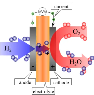
A fuel cell converts chemical fuel into electrical energy through a chemical re-action where a hydrogen containing fuel source reacts with an oxidising agent

which is usually oxygen from the air[1–3]. The difference between fuel cells and batteries is that a fuel cell produces electricity continuously as long as fuel and oxygen are provided. Whereas in batteries the chemicals are present inside the battery and react with each other to produce electricity.

All fuels cells contain an anode, a cathode and an electrolyte which sep-arates the anode and cathode. The hydrogen fuel is split into protons and

elec-trons using a catalyst at the anode. Oxygen is split at the cathode. Then de-pending on the type of electrolyte used either H+ diffuse to the cathode or O2− diffuse to the anode where they form water. The electrons generated at the an-ode flow in an external circuit where the electrical energy can be used. In this work we focus on when the electrolyte is a proton exchange membrane (PEM) where protons diffuse from the anode to the cathode. This is illustrated in figure

Figure 1.1: A schematic of a fuel cell with using a hydrogen fuel. Protons diffuse through a proton electrolyte membrane from the anode to the cathode where they react with oxygen to form water.

reactions are respectively,

H₂ → 2H++2e−

O2+4H++4e− → 2H2O

2H₂+O₂ → 2H₂O.

The energy contained in the molecular bonds are released in the form of elec-trons and little wasted in the form of heat in comparison to the conventional combustion engines which are used in modern vehicles. The incease is

approx-imately from 20% in combustion engines to over 40% in a PEM fuel cell. Thus there is huge potential for economics as well as incidental environmental bene-fits if PEM fuel cells are developed and brought into common use.

The first fuel cell powered by hydrogen and oxygen gas was created by William Robert Grove in 1839. He immersed ends of two platinum electrodes in a solution of sulphuric acid on one side and hydrogen or oxygen on the other.

voltaic" battery[4, 5].

In 1889 Ludwig Mond and Carl Langer created a fuel cell which ran on gas derived from coal instead of hydrogen as had been used until then[6]. They called this "Mond-gas" and it is notable for being the first use of a hydrogen

containing fuel which was not diatomic hydrogen.

In 1893 Friedrich Wilhelm Ostwald explained the performance of fuel cells. He determined the role each of the components of fuel cells and how it related to all the others. This included explaining function of the electrodes, electrolyte and oxidising and reducing agents[7]. His work in effect explained how Groves gas battery worked which until this point had been been unknown

and a topic of heated debate.

In 1933 Francis Thomas Bacon made an alkali based fuel cell which uses hydroxide as oxidant instead of oxygen[8]. This design was later developed by NASA for use in space due to its clean operation and the only end product being drinkable water. The result was a 1.5 kW "Apollo fuel cell" used in space on the Apollo missions between 1958-9[9].

In the 1950s fluorinated and sulfonated carbon chains become available for use as electrolyte membranes. In 1955 the first commercial fuel cell was made by Willard Thomas Grubb for General Electric (GE) [10]. It used a pro-ton exchange membrane of sulfonated polystyrene. Three years later in 1958 another GE scientist Leonard Niedrach succeeded in depositing platinum on the membrane to act as catalyst for the oxidation of hydrogen and reduction of

oxy-gen [10]. This fuel cell was also the PEM cell and it was used in the Gemini space missions between 1962 and 1965 to power the craft in space[9, 11].

In the 1970s scientist at DuPont built a fuel cell using a new flourinated polymer called Nafion as their proton electrolyte membrane. This polymer is still the most widely used today due to mechanical durability and conductivity[12] which no material since has been able to match commercially. However, like

other fluorinated polymers it relies on being hydrated by water for its proton conduction which limits its operating temperature to 80 °C[3].

(FCs) which are capable of replacing the internal combustion engine. The ad-vantage in power generation efficiency of fuel cells over conventional engines makes them ideal replacements in areas such as the transport industry,

dis-tributed power and portable electrical devices.

Today the main problems holding back the commercialisation of fuel cells in vehicles is the lack of an appropriate and cost effective electrolyte membrane. Most electrolytes operate at high temperatures of many hundred degrees. This is for obviously undesirable in a moving vehicle as such materials would need to be heated to their conducting temperature before operation. Polymer

elec-trolyte membranes have shown significant proton conductance in the intermedi-ate temperature regime of 150°C to 200°C[13,14]. These temperatures are also required as carbon monoxide (CO) poisons the platinum nanoparticle (Pt/C) catalyst used at the anode at lower temperatures[14–16]. This is because there is a large entropy associated with Gibbs free energy of CO adsorption onto Pt/C which can overcome the enthalpy of adsorption at high temperatures[16].

In addition to having a high proton conductivity the desired properties of

an ideal PEM for use in fuel cells include both long term structural and thermal stability of the proton conductivity. An anhydrous membrane which eliminates the need for water management systems which plagues the current Nafion based membranes. Any membrane also needs to be as inexpensive as possible to allow for use in mass production[13].

The amount of articles exploring one or more of these areas have

ex-ploded[17]. Recent developments in materials for PEMs involve immobilising heterocyclic aromatic compounds such as imidazole[18, 19], triazole[20, 21], pyrazole[22]and and benzimadole[20, 23]to a scaffold to improve their ther-mal and structural stability. These heterocycles posses all both hydrogen accep-tor (base) and donor (acid) sites and by analogy to water this is thought to be why they are good at forming hydrogen bonded networks which can be used

for proton transport. While the scaffolds successfully stabilise the heterocycles it comes at the cost of significantly reduced proton conductivity.

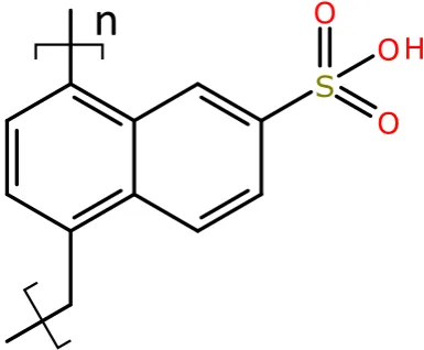
Formaldehyde (NSF) resin which is made up of polymerised naphthalene monomers with an acidic sulfonate group attached. The NSF resin adsorbed into the pores of mesoporous metal oxides to stabilise the polymer thermally and mechanically

as with the heterocycles. The sulfate acid is much stronger than the nitrogen based heterocycles but NSF does not have any groups which can act as proton acceptors. However, the walls of the pores in the Titanium, Tantalum and Nio-bium oxides used in this work are also acidic which means that they could also participate in proton conduction. It therefore the goal of this thesis to elucidate as far as possible the diffusion pathway of NSF resin adsorbed into the pores

of a metal oxide. Of particular focus how the metal oxide framework is able to enhance the proton conductivity of NSF resin observed in bulk[24, 25]and determining whether the pore walls participate in the proton transport.

1.1

Nuclear Magnetic Resonance of Proton Electrolyte

Membranes

It has been shown that proton conduction can occur via two distinct

mecha-nisms. The first is vehicle transport i.e. water molecules physically moving and bring protons along[26]. The second is Grotthus jumping or structural diffusion protons jumping between hydrogen bonding sites in a sample [26, 27]. These mechanisms are not mutually exclusive and it is well established that the high proton conductivity of water is higher than can be explained purely by vehicle

diffusion of H2O molecules. There is a significant contribution to the overall diffusion rate by structural diffusing protons between adjacent water molecules through the formation of hydroxyl (OH−) and hydroxonium (H3O+) [28–30]. As has been discussed water is not desirable in the PEM of a fuel.

Therefore there is impetus to understand rapid structural diffusion in or-der to help in the creation of an anhydrous material which can transport protons purely through structural diffusion. At its simplest structural diffusion is protons

de-pendent on the local structure for the availability of hydrogen bonding sites to jump between. It has been shown that a high density of hydrogen bonding sites which are dynamically connected meaning each site can be connected to several

others at different times yields increased proton motion. This enables proton motion to cascade into rapid diffusion[26, 31]. The local environments which protons experience as well as the dynamics of the motion vary greatly between samples.

Nuclear magnetic resonance provides a set of powerful tools to investi-gate all these aspects of proton transport at an inherently local level which dis-tinguishes it from other analytical tools such as diffraction. The principal way to

investigate motion using NMR involves identical experiments repeated at many different temperatures to observe the evolution of a particular property and then model this evolution.

The simplest parameter this is done with is the proton chemical shift which is extremely sensitive to changes in the local environment[32, 33]. This has been used to calculate the rate constant for proton transport between a

hy-drogen bonded and free state when participating in diffusion[34]. The change in the rate constant can then be used in an Arrhenius plot to calculate the energy barrier between these two states. However, this exact analysis is only possible in situations where there is symmetric exchange[34]. Nevertheless, this illustrates that the chemical shift carries much information about the dynamic processes which protons participate in[35, 36].

A closely related property when discussing proton transport is the width of the proton resonance which is inversely related to the T2 relaxation. The linewidth of the resonance is also directly related to the exchange rate between hydrogen bonded sites and thus proton diffusion. This is because motion aver-ages inhomogeneous magnetic fields over the period of the NMR experiment. This can again be modelled as random motion which must overcome a certain

The spin lattice T1 relaxation is likewise affected by motion of the dif-fusion protons. This can be modelled by assuming the only interaction which causes T₁ relaxation is the fluctuation in the proton homonuclear dipolar

cou-pling due to motion as it is much larger than any other interaction. This is called the BPP model and combined with the assumption that all motion causing relax-ation in this model has an associated characteristic frequency which is thermally activated and random. This means the the characteristic frequency of the mo-tion can be simulated using an Arrhenius relamo-tionship allows one to calculate the expected T₁ relaxation at a given temperature[36,44–48]. However, simulating

the the T1 data in most samples requires an empirical modification to the model which is called the stretched BPP[49, 50].

Diffusion rate can be measured using a technique called pulsed field gra-dient NMR[51]. In the case of proton conducting materials it has been used to measure the diffusion of water hydrated membranes with a fluoridated carbon polymer chain like Nafion[52, 53]and SPEEK[52]as well as molten phosphor

Chapter 2

NMR Theory

This chapter lays out the foundations of the quantum mechanical theory behind NMR including a description of the matrix formalism used to describe nuclear spins and their time evolution as well as the effect of the dipolar coupling and

how its line broadening effect may be eliminated. This chapter is based mostly on the books written by Abragam[59], Duer[60]and Callaghan[61].

2.1

Mathematical Description of an NMR

experi-ment

2.1.1

Nuclear Spin

Spinis an intrinsic property of matter in the same way as electric charge, mass or energy are properties of matter. The spin of a nucleus is determined by its constituent protons and neutrons. Spin is quantised in units ofħh (the reduced Plank constant) and its maximum value is dependent on the spin angular

mo-mentum quantum number, I, which can take a positive integer or half-integer

values.

perma-nent magnetic moment,µ, which interacts with any applied magnetic field,B0, whereby the degeneracy of the spin states is lifted. This is called the Zeeman

interactionand the energy shift it causes, denoted in classical terms, is,

E=₋µ_·B0. (2.1)

When this is expressed by quantum mechanical operators the result is the

Zeeman Hamiltonian, ˆHZ, given by,

ˆ

HZ =−ˆµ·B0 =−γħhˆI·B0, (2.2)

where γis the gyromagnetic ratio, ˆµ is the operator for the magnetic moment

and ˆI is the operator for the spin angular momentum. In NMR the applied magnetic field is described as an axial field along the z-axis in which case the Zeeman Hamiltonian becomes

ˆ

HZ =−γħhB0ˆIz, (2.3)

where ˆI_z the component of the spin angular momentum parallel to the z-axis. This equation is often written as,

ˆ

HZ =ω0ˆIz, (2.4)

where ω0 = −γB0 is called the Larmor frequency and ħh has been dropped re-sulting in units of angular frequency. The gyromagnetic ratio is a constant for a particular spin isotope which means each isotope has a characteristic Larmor

frequency under a particular field strength.

2.1.2

Angular Momentum Operators

represents the desired physical property. Using Dirac notation theexpectation

value,〈A〉, can be calculated

〈A〉=〈ψ|Aˆ|ψ〉. (2.5)

A spin system is described by the wavefunctions|I,m〉whereI is the spin angular momentum quantum number and m the magnetic quantum number. The operators representing spin angular momentum are ˆI_x, ˆI_y, ˆI_z and ˆI2. The

first three are components of the spin along the x, y andzaxes, while the latter is the total spin. The spin wavefunctions|I,m_〉are eigenfunctions of the ˆI_z and ˆ

I2 operators and are therefore referred to as the Zeeman eigenfunctions with their eigenvalues given by

ˆ

I2|I,m〉 = I(I +1)|I,m〉 (2.6)

ˆ

I_z|I,m〉 = m|I,m〉, (2.7)

where m can take values I,I −1, ...,−I for a total of 2I +1 states. The work presented in this thesis has used spins withI =1/_{2. Such spins have two states} which are commonly labelled|α〉(spin up) and|β〉(spin down), where follow-ing equation 2.7:

ˆ

I_z|α〉= +1₂|α〉 ˆI_z|β〉=−1₂|β〉. (2.8)

In order to completely describe a spin I = 1/_{2 quantum mechanically, a} linear superposition of its two states is used

|ψ〉=c_α|α_〉+c_β|β_〉, (2.9)

wherec_αandc_β are complex coefficients which determine the weighting of each state. Using equation 2.5, the expectation value for the ˆI_z operator is

〈ˆI_z〉 = c_αc_α∗_〈α_|ˆI_z|α_〉+c_αc_β∗_〈α_|ˆI_z|β_〉+c_βc_α∗_〈β_|ˆI_z|α_〉+c_βc_β∗_〈β_|ˆI_z|β_〉(2.10)

= 1

2(cαc

∗

However,|α〉and |β〉are not eigenfunctions of the ˆI_x and ˆI_y operators. Instead applying these operators leads to interconversion between the states.

ˆ_Ix|α〉=1

2|β〉 ˆIx|β〉=

1

2|α〉 and ˆIy|α〉=

i

2|β〉 ˆIy|β〉=−

i

2|α〉. (2.12)

The expectation values of the ˆI_x and ˆI_y operators therefore becomes

〈ˆI_x〉= 1₂(c_αc_β∗+c_βc_α∗) 〈ˆI_y〉= ₂i(c_αc_β∗−c_βc∗_α). (2.13) From equations 2.11 and 2.13 it can be seen that while the expectation value of the ˆI_zoperator is defined by the self-products of the coefficients, the ex-pectation values of ˆI_x and ˆI_y only contains the cross-products of the coefficients.

This fact allows the calculation of the expectation value in a more efficient no-tation as will be shown in the next section.

2.1.3

The Density Matrix and Operator

When a spin system is small, the linear combination of states is sufficient. How-ever, if there are several coupled spins or if I >1/_{2 then this notation becomes} unwieldy. Calculations become convenient by using a matrix notation instead.

An operator, ˆA, can be described by a matrix with elementsA_rs=〈r|Aˆ|s〉, where for a single spin withI =1/_{2thenr ands are both either}α_orβ_:

A=

‚

A_αα A_βα

A_αβ A_ββ

Π=

‚

〈α|Aˆ|α〉 〈β|Aˆ|α〉 〈α|Aˆ|β〉 〈β|Aˆ|β〉

Œ

. (2.14)

This is called thematrix representationof operator ˆAin the eigenbasis of ˆ

I_z.

Likewise the spin system can be described by a matrix, using thedensity

operator:

ˆ

ρ=|ψ〉〈ψ|, (2.15)

omit-ted for simplicity in the following. This gives rise to the density matrix with elementsρ_rs =〈r|ρˆ|s〉=〈r|ψ〉〈ψ|s〉 where for a single spin with I = 1/_{2 then}

|ψ〉is defined in equation 2.9 while randsremain defined as in equation 2.14:

ρ= ‚

ρ_αα ρ_βα ραβ ρββ

Π=

‚

c_αc∗_α c_βc_α∗ c_αc_β∗ c_βc_β∗

Œ

. (2.16)

It can be seen clearly that the effect of the density operator is to extract the coefficient of the state it operates on. This means the elements of the den-sity matrix are self-products and cross-products of the coefficients seen in the

expectation values of the angular momentum operators in equations 2.11 and 2.13. To extract these terms from the density matrix a matrix multiplication is performed with the matrix representation of the operator:

ρA = ‚

c_αc_α∗A_αα+c_βc_α∗A_βα c_αc_α∗A_βα+c_βc_α∗A_ββ

c_αc∗_βA_αα+c_βc_β∗A_αβ c_αc_β∗A_αβ+c_βc_β∗A_ββ

Œ

. (2.17)

The diagonal elements contained in the matrix above are the exact terms as in equation 2.10 used to calculate the expectation value of the angular

mo-mentum operators. The off-diagonal elements, however, are not relevant and therefore discarded. This is done formally by taking the trace of the matrix:

〈A〉=T r(ρA) =c_αc_α∗A_αα+c_βc_α∗A_βα+c_αc_β∗A_αβ+c_βc_β∗A_ββ. (2.18) The above equation contains the full expression for the expectation value of an angular momentum operator. However, the matrix representation of any operator contains several elements which are zero which significantly reduces the number of terms one needs to consider.

2.1.4

The Propagator

evolution of the precession generates a time varying signal, which is detected by induction using the spectrometer circuitry. In this context, it is appropriate to discuss the evolution with time of a spin ensemble, in the form of the density

operator, ˆρ(t), to describe the NMR signal.

The time evolution of any wavefunction, |ψ〉, can be described by the time dependent Schrödinger equation:

d

d t|ψ〉=−ıH |ˆψ〉, (2.19)

where Hˆ is the time independent Hamiltonian acting on the spin system. If a similar differentiation is applied to the density operator from equation 2.15, then the Liouville von-Neumann equation can be derived:

d

d t|ρˆ(t)〉=−ı

_ˆ

H, ˆρ(t), (2.20)

which has the standard solution:

ˆ

ρ(t) =e−ıHˆtρˆ(0)eıHˆt. (2.21) This is an extremely powerful equation which allows one to calculate the density matrix, and hence the state of the whole spin system, at any time. The

only requirements are that the initial state of the density matrix, ˆρ(0), and the Hamiltonian, Hˆ, acting on the system in the subsequent time are known. At thermal equilibrium, ˆρ(0) ∝ ˆI_z. The form of the Hamiltonian is discussed in more detail in the next section.

2.2

The Hamiltonian

a diamagnetic sample, the complete set of terms is:

ˆ

Ht ot al=HˆZ+HˆRF+HˆD+HˆQ+HˆJ+HˆC S, (2.22)

each of these Hamiltonians can be written in a completely general form:

ˆ

HΛ=ˆI·Λ˜·ˆS= ”

ˆ

I_x ˆI_y ˆI_z—



 

A_{x x} A_{x y} A_xz

A_{y x} A_{y y} A_yz

A_{z x} A_{z y} A_zz

      ˆ S_x ˆ S_y ˆ S_z  

, (2.23)

where ˜Λis a second rank tensor, ˆIis a spin operator and ˆScan be either another spin operator or an external field.

The simplest example of such a Hamiltonian is the Zeeman Hamiltonian, ˆ

HZ, which describes the interaction between the nuclear spin, ˆI, and the

exter-nal magnetic field, ˆB0, and is written as:

ˆ

HZ =ˆI·Z˜·Bˆ0, (2.24)

where

˜

Z=−γ



 

1 0 0 0 1 0 0 0 1





, (2.25)

whereγis the gyromagnetic ratio. The Zeeman Hamiltonian defines the geom-etry of the laboratory frame, which is the frame all other Hamiltonian tensors have to be expressed in relation to. In this frame, the external magnetic field

is aligned with the z-axis such that ˆB0 =

0 0 ˆB₀. Likewise, the magneti-sation of the spins in this frame is also aligned with the z-axis and therefore ˆ_{I =}

0 0 ˆI_z. This results in the familiar Zeeman Hamiltonian from section 2.1.1:

ˆ

2.2.1

Spherical Tensors

For each of the Hamiltonians in equation 2.22, there is a principal axis frame (PAF) in which the second rank tensor, ˜A, in equation A.1 only has diagonal ele-ments which are non-zero. The PAF is, however, not coincident with the labora-tory frame, defined by the Zeeman Hamiltonian, and from which one observes the spin system experimentally. The PAF is, because of its diagonal tensor, the preferred frame to use. However, interaction tensors in the PAF have to undergo

a frame rotation to bring them into the laboratory frame. This transformation is necessary because the effect of the interaction has no physical meaning unless it is expressed in the frame which it is observed from.

Cartesian tensors are a nuisance to perform frame rotations on as after just one rotation it very likely that all nine tensor elements are non-zero. It is instead convenient to use a set of basis operators with spherical symmetry, the

irreducible spherical tensor operators. Irreducible spherical tensors, ˆT_j, have a

rank j=0, 1, 2, ... and each contain operator elements, ˆT_j,m, which are labelled

with an orderm= j,j₋1, ...,−j. All the spherical tensors up to and including rank j=2 are shown in Appendix A.

The elements of a tensor with rank jform a complete set under rotation, i.e., elements with different ranks do not mix. This is due to irreducible spherical

tensor operators transforming like the irreducible representation of the three dimensional rotation point group and it greatly reduces the number of non-zero elements obtained after a rotation. The Hamiltonian of interaction Λ can be written as a sum of several irreducible spherical tensor operators:

ˆ

HΛ=

2 X

j=0

+j

X

m=−j

(−1)m_A

j,mTˆj,−m, (2.27)

whereA_j,mdescribes the orientation dependence of the interactionΛ, while ˆTj,−m

are the appropriate operators for the spin component of the interaction.

irreducible spherical tensor are non-zero:

ˆ

HPAF_Λ =APAF_0,0 Tˆ_0,0+APAF_2,0Tˆ_2,0+APAF_2,2 Tˆ_2,−2+APAF_2,−2Tˆ_2,2. (2.28) In addition, some Hamiltonians have even fewer terms contributing due to addi-tional symmetry elements in the interaction. For example, the dipolar coupling, which will be discussed in more detail later, only has a single non-zero tensor element, ˆH PAF_D =APAF_2,0 Tˆ_2,0.

2.2.2

Frame Transformations

The transformation from the principal axis frame, Hˆ_ΛPAF, into the laboratory frame, ˆH_ΛLAB, is performed via three successive rotations through the Euler an-gles(α β γ)about the axes in the original PAF. The full rotation, ˆR(α,β,γ), is described in terms of each rotation individually:

ˆ

R(α,β,γ) =Rˆz(γ)Rˆy(β)Rˆz(α), (2.29)

where ˆR_a(θ)is a rotation about the axis a by an angle θ and it can be shown that it takes the form

ˆ

R_a(θ) =exp(−ıθˆI_a). (2.30)

For an irreducible spherical tensor, the equivalent frame transformation

is performed using a rotation matrix of the form

D_mj0,m(αβγ) =exp(−ım0α)d

j

m0,m(β)exp(−ımγ), (2.31)

where d_mj_0,m(β) is a reduced Wigner rotation matrix element. A rotation from a starting frame, APAF_{, to an end frame, A}LAB_{, using the rotation operator with}

form

ALAB_j,m0=X

m

APAS_j,mD_mj_,m0(αP L,βP L,γP L), (2.32)

whereby the Hamiltonian of the interaction in the laboratory frame becomes

ˆ

H_ΛLAB=

2 X

j=0

+j

X

m=−j

(−1)m_Tˆ

j,−m

X

m0

APAS_j,m0D

j

m0,m(αP L,βP L,γP L). (2.33)

This description only holds for static samples. In order to take into ac-count the effect of magic angle spinning, an intermediary frame, therotor frame, needs to be introduced. This will be discussed in section 2.4.

2.2.3

The Secular Approximation

Of all the terms contributing to the complete Hamiltonian in equation 2.22 the

Zeeman Hamiltonian, HˆZ, is the strongest. The rest of the interactions have

Hamiltonians

ˆ

H1=HˆRF+HˆD+HˆQ+HˆJ+HˆC S, (2.34)

which can be well described as a small perturbation on the Zeeman Hamilto-nian. If this is the case then the eigenfunctions of ˆH1are well approximated by the eigenfunctions of the Zeeman Hamiltonian. Limiting the situation to when

ˆ

H1 is purely described by the Zeeman eigenfunctions, which is a first order approximation, then the following holds.

Since ˆH1and ˆHZhave the same eigenfunctions they must also commute.

This means only the parts of ˆH1 which actually commutes with ˆHZ can affect

two operators is

[ˆ_{Iz, ˆTj,m] =mT}ˆ_{j,m. (2.35)}

Therefore, the only irreducible spherical tensors which can affect the Zee-man energy levels are those with an order ofm=0, as only under this circum-stance do the operators commute. It must be noted that this is only true when examining the interactions in the laboratory frame. In this frame, using the

secular approximation, only two tensors contribute to a Hamiltonian:

ˆ

H_ΛLAB=ALAB_0,0 Tˆ_0,0+ALAB_2,0 Tˆ_2,0. (2.36)

2.3

Effect of Radio Frequency Pulses

A radio frequency pulse affects the spin system like a oscillating magnetic field, B1(t). As the magnetic field affecting the spin system is time dependent so are the resulting eigenstates and energies. A standard NMR probe can deliver a radio frequency pulse equivalent to an oscillating magnetic field B₁ of

approxi-mately 1 mT. This is several orders of magnitude less than a static magnetic field which is typically on the order of 10 T. This means that any RF field will have no effect on the spin states unless it is on resonance with the Larmnor frequency. In equation 2.2 we described the Zeeman Hamiltonian and we now add this oscillating magnetic field

ˆ

H = HˆZ +Hˆpulse

= −γB₀ˆI_z−2γB₁(t)ˆI

= ω0ˆIz+2ωnutcos(ωr ft+φ)ˆIx (2.37)

where the carrier wave of the oscillating magnetic field isωr f with phaseφand

transforming into a frame which is rotating around the z-axis at the frequency

ωr f using the rotation operator in equation 2.30 and applying it to the

Hamil-tonian in the following fashion:

ˆ

Hr ot = ˆRz(−ωr ft)HˆˆRz(+ωr ft)

= ˆ_{Rz(−ωr ft) H}ˆ_Z+Hˆ_pulseˆ

R_z(+ω_{r f}t). (2.38)

As the ˆI_z operator is invariant under rotation around the z-axis we only need to consider the effect on ˆHpulse. Thus in the rotating frame the Hamiltonian

for the RF pulse becomes

ˆ

Hpulse,r ot = ˆRz(−ωr ft)HˆpulseRˆz(+ωr ft)

= −ωr fˆIz+ωnut ˆIxcosφ+ˆIysinφ

. (2.39)

We can now choose the phase of the RF pulse to beφ =0 without any loss of generality and this yields the following form for the Hamiltonian in the rotating frame

ˆ

Hr ot = HˆZ +Hˆpulse,r ot

= ω0ˆIz−ωr fIˆz+ωnutˆIx. (2.40)

As previously stated the static magnetic field giving rise to the Larmor frequency, ω0, is much larger than the magnetic field caused by the oscillating magnetic field ω_nut. However, if we choose the carrier frequency, ω_{r f} of the oscillating magnetic field to beon resonancewith the Larmor frequencyω_{r f} =ω₀

the effect of the static magnetic field is canceled and the Hamiltonian acting under these circumstances simply becomes

ˆ

Hr ot =ωnutˆIx. (2.41)

which describes the effect of a Hamiltonian through time

ˆ

ρ(t) =e−ıωnuttˆIxˆ_I

zeıωnutt

ˆ

Ix _(2.42)

By comparison to the rotation operators in equation 2.30 it is clear that this equation describes a rototation of the initially longitudinal magnetisation around the x-axis which generates transverse magnetisation along the y-axis

ˆ

ρ(t) =ˆI_zcosωnutt−ˆIysinωnutt. (2.43)

It is clear that we can choose how much of the magnetisation we transfer from the z-axis to the y-axis by changing the duration,τ_{r f} of the applied pulse

with nutation frequencyωnut

θnut =ωnutτr f (2.44)

For a pulse were the entire magnetisation is rotated to the y-axis this

becomesωnutτr f =π/2 and we speak of a 90°-pulse. Similarly, a pulse where

ωnutτr f =πis called a 180°- pulse.

This description of the RF pulse is still viewed from the rotating frame. If we briefly consider the view from the laboratory frame we observe that during the duration of the RF pulse the magnetisation still precesses around the z-axis while the magnetisation is simultaneously rotated around the x-axis. This type

of rotation is callednutation.

2.3.1

NMR Signal Detection

When considering an ensemble of spins it is clear that the effect of the 90◦_x-pulse described is entirely coherent magnetisation along−ˆI_y. For a spin 1/2 such a magnetisation is in fact an equal mixing of the|α〉and|β〉states of the Zeeman

Zeeman Hamiltonian

ˆ

ρ(t) =−ˆI_ycosω0t+ˆIxsinω0t. (2.45)

This describes magnetisation rotating clockwise around the z-axis in the transverse plane at the Larmor frequency which induces an electromotive force (EMF) in the coil used to generate the RF pulse. This is called thefree induction

decayor FID and is the manner in which the NMR experiment is detected.

This detection is actually achieved by mixing the signal measured at the Larmor frequencyω0 with a reference frequencyωo bs. The effect of this can be

seen by entering a frame rotating atωo bs

ˆ

ρr ot(t) =−ˆIycos(ω0−ωo bs)t+ˆIxsin(ω0−ωo bs)t. (2.46)

The complex signal operatorNγ[ˆI_x+ıˆI_y]is then used to extract the signal which is observed

T r(Nγ[ˆI_x+ıˆI_y]ρˆ_{r ot}(t)) = − ıTr(ˆI2_y)cos(ω0−ωo bs)t

+ Tr(ˆI2_y)sin(ω0−ωo bs)t, (2.47)

where the trace is used to remove unobservable off diagonal elements.

Using the identity

Tr(ˆI_x2) =Tr(ˆI2_y) =Tr(ˆI_z2) = 1

3I(2I+1)(I+1) (2.48)

and the equilibrium magnetisation

M_eq= Nγ

2_B

0ħh2I(I +1)

3k_BT (2.49)

simply write the expected observed signal as

T r(Nγ[ˆI_x+ıˆI_y]ρˆ_{r ot}(t)) =ıM_eqexp(−ı(ω₀−ωo bs)t) (2.50)

This result is important as one can measure a signal from the EMF in this form using a method called RF heterodyne detection. In such a detection scheme the signal output of the RF coils which is in the form V₀cosω₀t is split

into two channels where it is mixed separately with a reference frequency which is 90°out of phase with each other by which is obtained separate in phase and quadrature phase output signals. Heterodyning with two quadrature channels is equivalent to multiplication

V₀cosω0t(cosωt+ısinωt)

= V0cosω0texp(ıωt)

= V₀[exp(−ı(ω₀₋ω)t) +exp(ı(ω₀+ω)t)]. (2.51)

It is clear that the first term in equation 2.51 is equivalent to equation 2.50 and therefore this method is capable of measuring the operators ˆI_x +ıˆI_y.

The fact that we also measure the frequency sum is irrelevant as it can be easily eliminated using a filter.

2.4

Magic Angle Spinning

All interactions described by second rank tensors such as the dipolar coupling and the chemical shift have anisotropic components which affect the observed frequency depending on the molecular orientation relative to the applied B0 magnetic field. In a powdered sample where all possible orientations may be assumed to be present this results in broadpowder pattern lineshape. This gives

in-clined by an angleβ_RL. This can be treated mathematically using the methods described in section 2.2.2 by inserting an intermediary rotating frame, the rotor frame, between the PAF and the laboratory frame. In order to understand the

effect of MAS on any second order interaction such as the dipolar coupling or the chemical shift one need only consider the following tensor element,

ˆ

HPAF_D =APAF_2,0Tˆ_2,0. (2.52)

In order to transform into the rotor frame, the PAF is rotated through the Euler angles (α_PR β_PR γ_PR). Written in the form of equation 2.32, the transformation becomes:

Ar ot or_2,m =APAS_2,0D_0,2_m(α_PR,β_PR,γ_PR), (2.53)

where m = 0,±1,±2 for a total of five terms. Note that the order, m, does not have to be zero, as it is not necessary to fulfil the secular approximation because this is not the laboratory frame. To reach this frame, another rotation through the Euler angles (_{αRL βRL γRL}) is necessary. Here the angleα_RL

de-scribes the continual rotation of the intermediary rotor frame relative to the laboratory frame such thatαRL =−ωRt, whereωR is the rotation frequency in

angular frequency units andγPRis the rotor phase relative to the magnetic field

which defines the initial orientation of the interaction.

ALAB_2,0 =

2 X

m=−2

APAF_2,0 D_0,2_m(α_PR,βPR,γPR)Dm2,0(αRL,βRL,γRL) (2.54)

= 2 X

m=−2

APAF_2,0d_0,2_m(β_PR)d_m2_,0(β_RL)exp(−ımγ_PR)exp(−ımα_RL), (2.55)

whereALAB_2,0 is the only term in the laboratory frame due to the secular approxi-mation which now applies. When equation 2.55 is written in full, it becomes:

ALAB_2,0 =APAF_2,0



 

1 4

3 cos2βPR−1 3 cos2βRL−1

−3₄sin 2βPRsin 2βRLcos[γPR−ωRt]

+3

4sin

2_β

PRsin2βRLcos[2γPR−2ωRt]





The inclination of the rotor frame relative to the laboratory frame,β_RL, is under experimental control and when it is set toβ_RL =54.74◦, the 3 cos2_β

RL−1

term equals zero and equation 2.56 reduces to:

ALAB_2,0(t) =APAF_2,0

‚

−p1

2sin 2βPRcos[γPR−ωRt]

+1

2sin

2_β

PRcos[2γPR−2ωRt]

Œ

. (2.57)

Every term describing the spatial dependency of the second rank tensor is now time dependent. The integral of equation 2.57 over a full rotor period

∆t=τ_R=2π_/ω

Ris zero:

Z τR

t=0

ALAB_2,0(t)d t=0. (2.58)

Equation 2.58 is interpreted as the time dependent part of the second rank tensor being averaged to zero over a full rotor cycle. However, the evolution during the free induction decay is often sampled more than once over a rotor cycle, and may therefore not be completely averaged to zero. This leads to the observation of spinning sidebands, if the spinning frequency is low compared

to the magnitude of an interaction such as the dipolar coupling or chemical shielding.

2.5

Chemical Shift

The behaviour of the nucleus in reaction to an external magnetic field is the primary interest in NMR. However, the electrons which surround every nucleus are also affected by the external magnetic field of the NMR spectrometer. The electrons react to produce a secondary field which modifies the the total mag-netic field experienced by the nucleus in a manner which depends on the local electron distribution. The interaction between this secondary magnetic field and

Firstly, all electrons affected by the external magnetic field are subject to the Lorentz force. For bound electrons this induces a current as they move within their orbitals. This motion causes a secondary field which opposes the external

field at the centre of motion. The total magnetic field which is experienced by the nucleus is therefore reduced by the electron motion. This is called a shield-ing interaction and is known as the diamagnetic contribution. The strength of the interaction depends on the distance between the electrons and the nucleus. The dependence is of the order of 1/r3_{, where r is the radial distance between} the nucleus and electrons. Consequently, the core electrons being closest to the

nucleus contribute more than valence electrons which are further from the nu-cleus. This effect therefore tends to be fairly constant for a particular type of nucleus. However, the diamagnetic current at any one nucleus are affected by the surrounding atoms which each generate their own currents. The total effect of these diamagnetic currents on the NMR frequency is observed by changing the Larmor frequency of a given nucleus depending its local environment. This

is the primary effect which causes the chemical shift.

Secondly, the external magnetic field distorts the ground state electron or-bitals which determine the electron density distribution around a nucleus. This distortion of the ground state can be described as a perturbation of ground state by orbitals of a higher energy excited electronic state. These excited electronic states can be paramagnetic and therefore cause the resulting ground electronic

state in an external magnetic field to slightly paramagnetic. The result of such a paramagnetic state is to create a secondary magnetic field which supports the external field and is therefore said to deshield the nucleus.

Importantly both these components are affected by changes in the lo-cal electronic density distribution and geometry. The resulting chemilo-cal shift is therefore highly dependent on the local electronic environment. This makes the

chemical shift extremely valuable to an NMR spectroscopist as it is diagnostic of the local electronic density and hence structure.

of an external magnetic fieldB0is written

ˆ

HC S =−γˆI·σ·B0, (2.59)

whereσ is a second rank Cartesian tensor called the chemical shielding tensor. The chemical shielding tensor can be diagonalised by choosing the correct prin-cipal axis frame. In this PAF the diagonal elements are frequently expressed as the isotropic shift,δ_iso, anisotropy,∆, and asymmetry,η, which are defined as

follows

σiso =

1

3 σx x+σy y+σzz

(2.60)

∆ = σzz−σiso (2.61)

η = σx x+σy y

∆ . (2.62)

These diagonal elements are commonly ordered and labeled as σ_zz − σiso≥σx x−σiso ≥σy y−σiso. This is called the Haeberlen convention[62].

A typical sample used in solid state NMR is powdered. Such a sample

contains many crystallites which have all possible orientations relative to the ex-ternal magnetic fieldB0. Crystallites at each orientation give rise to a frequency

shift. When the resonances of all crystallites at all orientations are co-added this yields a broad resonance called a powder pattern.

NMR experiments do not measure the chemical shift directly. Rather, the a reference compound is used and the frequencies of all resonances are mea-sured relative to a specific resonance in spectrum of the reference. Therefore

any chemical shifts quoted are offset frequencies relative to specific resonance in a specific compound and calculated using the following equation

δiso=

ν−νr e f

νr e f

, (2.63)

whereδ_iso is the isotropic chemical shift in units of parts per millionorppm.

shield-ing which are discussed by Duer [60] but these are outside the scope of this work.

2.5.1

Under MAS

The anisotropies giving rise to a powder patterns which are recorded in static NMR experiments contains much information. However, in a spectrum con-taining more than a couple of resonances the patterns tend to overlap which ob-scures any useful information. The chemical shielding interaction,σ, is a second rank tensor and as discussed in section 2.4 any anisotropic components arising from the interaction can be averaged to zero over a rotor period by spinning the

sample around the magic angle. For each resonance where the MAS frequency is smaller than the anisotropy this results in the observation of a series spin-ning sidebands separated by the spinspin-ning frequency where the solid resonances would have been.

2.6

Dipolar Coupling

The dipolar coupling is the interaction between the permanent magnetic mo-ments of two spins. It is a through space interaction, the magnitude of which depends on the orientation of the internuclear vector relative to the applied magnetic field,B₀. It is described by ˆHD, the dipolar Hamiltonian:

ˆ

HD=−2

X

i<j

ˆ_Ii·D˜_·ˆ_S

j, (2.64)

where ˆIi and ˆSj refer to theithspin of isotope I and the jth spin of isotopeS,

re-spectively. WhenI andSrefer to spins of the same isotope then the interaction is calledhomonuclearand when they refer to different isotopes then the interaction is calledheteronuclear. The interaction tensor ˜Dfor the dipolar coupling has the particularity that in the PAF the trace of the matrix is zeroA_{x x}+A_{y y}+A_zz=0 and

spherical tensor element contributing to the Hamiltonian in this frame

ˆ

HPAF_D =APAF_2,0Tˆ_2,0, (2.65)

where

APAF_2,0 =p6b_{i j}, (2.66)

and b_{i j} is the dipole coupling constant (in rad s−1) between the ith I spin and the jth S spin given by

b_{i j} =_ħh

µ 0 4π

γ

IγS

r_{i j}3 , (2.67)

whereµ0 is the permeability of free space and γI and γS are the gyromagnetic

ratios of isotopesIandSrespectively, whiler_{i j}refers to the internuclear distance between spiniand j. Note that, for convenience, the dipolar coupling constant is here defined as positive, whereas it is often defined as a negative number. In units of Hz, the dipolar coupling constant becomes,

d_{i j} =b_{i j}/2π. (2.68)

Using equations 2.31 and 2.32 to transform equation 2.65 from the PAF into the laboratory frame by rotating through the Euler angles(_{αP L βP L γP L}):

ALAB_2,0,st at ic = APAS_2,0D_0,02 (α_{P L},βP L,γP L)

= APAS_2,0d_0,02 (β_{P L})

= p

6b_{i j}1

2

3 cos2(β_{P L})−1 (2.69)

het-eronuclei:

ˆ

T_2,0H E T = 2ˆI_zSˆ_z (2.70)

ˆ

T_2,0HOM = 2ˆI_zSˆ_z−(Iˆ_xSˆ_x +ˆI_ySˆ_y) (2.71)

= 2ˆI_zSˆ_z−1

2(ˆI−Sˆ++ˆI+Sˆ−) (2.72) = 3ˆI_zSˆ_z−ˆI·ˆS, (2.73)

where ˆI_+,−=ˆI_x±ıˆI_y and ˆS_+,−=Sˆ_x±ıSˆ_y are the raising and lowering operators. In all the above equations a normalisation factor of p1

6 has been omitted and the matrix representations of the operators for a pair of spinI = 1₂ are:

2ˆI_zSˆ_z =

      1

2 0 0 0

0 −1

2 0 0

0 0 −1

2 0

0 0 0 1 2      

−(ˆI_xSˆ_x +ˆI_ySˆ_y) =

     

0 0 0 0 0 0 1

2 0

0 1

2 0 0

0 0 0 0

      . (2.74)

2.6.1

Heteronuclear Coupling

For the heteronuclear case, only the 2ˆI_zSˆ_z term is present and contains only di-agonal elements. Therefore the eigenstates of spins coupled by dipolar coupling are just products of the Zeeman eigenstates(|αα〉,|αβ〉,|βα〉,|ββ〉). It is pos-sible to calculate the expectation value of the first order shift in energy which

the Zeeman eigenstates experience, away from the Larmor frequency, when the dipolar coupling is taken into account:

〈m_Im_S|2ˆI_zSˆ_z|m_Im_S〉=2m_Im_Sd0, (2.75) whered0=d_{i j}1₂3 cos2(βP L)−1

.

For a pair of spin I =1₂ nuclei, this becomes,

|αα〉=|ββ〉= +1₂d0 (2.76)

The result of all of the above is that the NMR signal detected from the spins changes from the Larmor frequency to a distribution of frequencies centred on the Larmor frequency given by

νD(β) = ν0±d0

= ν0±di j

1 2

3 cos2(β)−1, (2.78)

the angleβ, being unevenly distributed between 0 andπin a powdered sample, gives rise to an additional weighting of sinβ. The result is a broad resonance with a particular shape called a Pake doublet[63].

2.6.2

Homonuclear Coupling

When two homonuclear spins interact, the additional term of ˆI_xSˆ_x+ˆI_ySˆ_y com-plicates matters. As can be seen in equation 2.72 this term can also be written as a combination of ladder operators, the effect of which is to mix the|αβ〉and

|βα〉eigenstates. The same is clear from the matrix representation in equation 2.74 which has two off diagonal elements which cause precisely this mixing. The

effect is that the eigenstates of the dipolar Hamiltonian are no longer products of Zeeman eigenstates but linear combinations of them.

Furthermore, consider a three spin system, where one of the possible eigenstates consists of a linear combination of the|ααβ〉,|αβα〉and|βαα〉 Zee-man eigenstates. If an observation is made of a system in this state, it collapses into one of the Zeeman eigenstates. If repeated measurements are made then

each of the Zeeman eigenstates will be seen at different times. If focussing on just one of the spins,I₁, then it would sometimes appear to be in state|α〉(when collapsed into |ααβ〉 or|αβα〉) and sometimes state|β〉(when collapsed into

|βαα〉). Therefore, it appears as if I1 is constantly changing its spin state be-tween|α〉and|β〉without the emission or absorption of a photon, as would be required if it were uncoupled. This is equivalent to there being a continuous

coupling by magic angle spinning as has been discussed in section 2.4.

When there are more than two homonuclear spins, the flip-flop term mixes degenerate Zeeman eigenstates, such that the resulting eigenfunctions for the full multiple spin system are linear combinations of the Zeeman

eigen-states, which are not degenerate. This gives rise to multiple different transition frequencies, which when observed under static conditions gives rise to a large broadening. The lineshape becomes approximately Gaussian, when there are many coupled spins. This is calledhomogenousbroadening.

2.6.3

Heteronucleus coupled to a homonuclear network

Finally, consider the effect of a large number ofIspins in a homonuclear network coupled to just one heteronucleusS. Suppose that a single spin, I₁, is closer to S than any other spin in the homonuclear network and therefore this pair also has the strongest heteronuclear dipolar coupling. From the discussion above, it is clear thatI1changes its spin state each time the system is observed. It should also be obvious that the magnitude of heteronuclear dipolar coupling depends

on which eigenstate both S and I₁ are in. Hence, when repeatedly observing spinS, the associatedS−I₁ dipolar coupling varies with each observation, as the heteronuclear dipolar coupling still depends on the ever changingI₁state. In such a case, homogeneous broadening, similar to that which would be observed on theI1spin, is also present in a spectrum showing theSresonance. Therefore, when observing theS spin it is necessary to include the network of I spins in

the description. This poses a problem when simulating spins in this situation as adding extra spins increases computation time exponentially.

2.6.4

Under MAS

Reducing the line broadening effect of homonuclear dipolar coupling between more than two spins is different to the case of a heteronuclear coupling of

between Zeeman eigenstates |α〉 and |β〉. The rate of change between eigen-states of a spin, I1, is equal to the strength of the dipolar interactions affecting

I₁ in frequency units. As MAS only averages the dipolar coupling to zero over a full rotor period, the spin state is required to remain unchanged in this time frame. Hence, to average the line broadening effect of a homonuclear dipolar coupling, the spinning frequency needs to significantly exceed the magnitude of the coupling being averaged. By contrast, it is possible to eliminate the line broadening effect of a heteronuclear dipolar coupling, when the spinning fre-quency is smaller than the size of the heteronuclear interaction.

2.7

Longitudinal Relaxation

The thermal equilibrium of a spin system was shown to be proportional to ˆI_z in equation 2.4. In equation 2.43 it was shown that this equilibrium magnetisation

can be converted into transverse magnetisation in the xy plane by the application of a RF pulse. The process by which magnetisation returns to its equilibrium state along ˆI_z is called longitudinal relaxation or spin-lattice relaxation and has a characteristic time constant T1.

Relaxation can be caused by anything which causes fluctuations in the lo-cal magnetic field through the molecular motion. In solid state NMR this motion

tends to be forms of reorientation such as methyl rotation or chemical exchange such as self diffusion of hydrogen bonded protons. The causes of such fluctua-tions in the local field are the anisotropic interacfluctua-tions of the chemical shielding (see section 2.5), dipolar coupling (see section 2.6), quadrupolar moment (see section 2.9) and paramagnetism.

This work is focused mainly on the relaxation rate of self diffusing protons

in organic polymers and metal oxide frameworks (MOFs). Under such circum-stances the dominant interaction causing fluctuations in the magnetic field is the homonuclear dipolar coupling between protons.

magnetisation are suddenly subjected to a static magnetic field,B0 the magneti-sation along the z-axis is given by

M_z(t) =M_eq 1−e−t/T1_{, (2.79)}

where M_z is the magnetisation along the z-axis after a time t and M_eq is the magnetisation along ˆI_zat equilibrium and T₁is the time constant describing how fast the magnetisation returns to the equilibrium state. Relaxation for a period

of t=T₁ results in∼63% of the equilibrium magnetisation aligned with the z-axis while after a period oft=5T_1∼99.3% of the equilibrium magnetisation is aligned. This is important as if NMR measurements are repeated faster than the longitudinal relaxation returns the magnetisation to the equilibrium state one risks saturating the spins and consequently not generating the coherence one

wishes to measure.

2.7.1

The Saturation Recovery

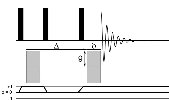
The saturation recovery experiment is an NMR experiment designed to measure the T1 longitudinal relaxation. The sequence and coherence transfer pathway for this experiment is shown in figure 2.1.

The sequence begins with a series of high power pulses called a pulse

comb. These pulses destroy all population differences between the Zeeman en-ergy levels or coherences generated by previous RF pulses. The spins can be considered to be completely randomly distributed as if there were no external magnetic field affecting them.

After the pulse comb there is a period,τ1, wherein the spin ensmble be-gins to relax back to its equilibrium state along the z-axis. The rate at which this

happens in given in equation 2.79.

t

pulse comb

p = 0 +1

-1

t

Figure 2.1: The pulse sequence for a saturation recovery experiment (top) and

its coherence transfer pathway (bottom). The black rectangles are RF pulses while the duration between pulses are periods of free precession.

This means that the magnitude of the signal detected in this case depends on how big a proportion of the spin have relaxed back to align with the z-axis. By varying the timeτ₁ the proportion of spin which are aligned with the z-axis

changes. The longerτ1 the higher the proportion of spins aligned and thus the signal intensity increases. Eventually, after a long relaxation periodτ1the spins reach their equilibrium magnetisation again and the signal intensity detected by NMR reaches a plateau. By repeating the experiment in figure 2.1 at different values ofτ1an NMR spectroscopist is able to measure the longitudinal relaxation rate, T₁, using the Bloch equations 2.79 to simulate the signal intensity recovered

after a period,τ1.

2.7.2

The BPP model

The classic paper by Bloembergen, Pound and Purcell (BPP)[65] describing a theoretical framework linking the random fluctuations in the local magnetic field caused by the dipolar fields of spins in motion in the sample. Importantly for this work, it describes how the relaxation reacts to changes in temperature.