Towards optimality of the parallel tempering algorithm

(1)

warwick.ac.uk/lib-publications

A Thesis Submitted for the Degree of PhD at the University of Warwick

Permanent WRAP URL:

http://wrap.warwick.ac.uk/99796

Copyright and reuse:

This thesis is made available online and is protected by original copyright.

Please scroll down to view the document itself.

Please refer to the repository record for this item for information to help you to cite it.

Our policy information is available from the repository home page.

(2)

Towards Optimality of the Parallel Tempering

Algorithm

by

Nicholas Tawn

Thesis

Submitted to the University of Warwick

for the degree of

Doctor of Philosophy

Department of Statistics

(3)

Acknowledgments

My supervisor, Gareth Roberts, has been integral in providing me with both

excel-lent guidance and essential support throughout the entirety of my PhD. His

inspi-rational input and assistance was truly appreciated.

Throughout my time at Warwick there have been many supportive friends

and colleagues who have really added to my understanding and enthusiasm for

statistics. There are too many to list but some key people who deserve a special

mention of thanks are: Jeff Rosenthal (University of Toronto); Paul Fearnhead

(University of Lancaster); Adam Johansen (University of Warwick); Murray Pollock

(University of Warwick); Matt Moores (University of Warwick) and Jon Warren

(University of Warwick).

Also I would like to acknowledge the financial support received from

EPSRC-Engineering and Physical Sciences Research Council.

I certainly couldn’t have done this without the love, care and support of both

my family and fianc´e Jen. Jen has been there to support, care and motivate me

through the most difficult periods of the PhD process; her unwavering optimism

has been fundamental to my completion of the thesis. Both my parents have been

incredible with their support throughout. I am grateful that they have constantly

been there to give the ultimate level of support to me throughout my life and I have

needed that more than ever during the PhD. I would like them to know how grateful

(7)

Declarations

I declare that the work and research contained in this thesis is my own unless

otherwise stated. This thesis has been submitted to the University of Warwick only,

and not to any other institution, in support of my application for the degree of

Doctor of Philosophy.

Signed:

(8)

Abstract

Markov Chain Monte Carlo (MCMC) techniques for sampling from com-plex probability distributions have become mainstream. Big data and high model complexity demand more scalable and robust algorithms. A famous problem with MCMC is making it robust to situations when the target distribution is multi-modal. In such cases the algorithm can become trapped in a subset of the state space and fail to escape during the entirety of the run of the algorithm. This non-exploration of the state space results in highly biased sample output.

Simulated (ST) and Parallel (PT) Tempering algorithms are typically used to address multi-modality problems. These methods flatten out the target distribution using a temperature schedule. This allows the Markov chain to move freely around the state space and explore all regions of significant mass.

This thesis explores two new ideas to improve the scalability of the PT algo-rithm. These are implemented in prototype algorithms, QuanTA and HAT, which are accompanied by supportive theoretical optimal scaling results.

QuanTA focuses on improving transfer speed of the hot state mixing informa-tion to the target cold state. The associated scaling result for QuanTA shows that under mild conditions the QuanTA approach admits a higher order temperature spacing than the PT algorithm.

HAT focuses on preserving modal weight through the temperature schedule. This is an issue that can lead to critically poor performance of the PT approach. The associated optimal scaling result is useful from a practical perspective. The result also challenges the notion that without modal weight preservation tempering schedules can be selected based on swap acceptance rates; an idea repeatedly used in the current literature.

(9)

Chapter 1

Introduction

1.1 Introduction

The Bayesian approach for inference on ad-dimensional parameterxcombines prior knowledge, in the form of a fully specified prior distribution, with information from

observed data y, incorporated through the likelihood function, to obtain a fully

specified posterior distribution ofx giveny, Note the unusual use of xrather than,

e.g.θ, as the notation for the parameter vector; this is for the sake of consistency

with all chapters in the thesis. Letting π(x|y) denote the posterior, f(y|x) the likelihood function,π(x) the prior distribution forx and f(y) the joint distribution of the data, then the posterior is computed using the standard Bayes formula:

π(x|y) = f(y|x)π(x)

f(y) ∝f(y|x)π(x). (1.1)

This posterior distribution is typically intractable with the joint distribution of the

data, f(y), typically unknown. Tractable models can be constructed using notions

of conjugacy with regards to prior distribution choice, but this defeats the object of allowing genuine expert judgment to be incorporated properly. Furthermore, the

use of conjugacy is only possible in a small subset of problems.

Indeed a practitioner is typically interested in expectations of some quantity, h(X), with respect to the posterior distribution, i.e.

Ex|y[h(X)] =

Z

x∈X

h(x)π(x|y)dx. (1.2)

Due to the intractability of the posterior, computational methods are required.

Indeed this Bayesian specific issue falls into a wider class of general problems

(10)

known up to a constant of proportionality but one wants to evaluate integrals of the

form

Z

x∈X

h(x)π(dx).

A class of methods with proven success in these settings is the Monte Carlo approach. Markov Chain Monte Carlo (MCMC) is one such method that has been

successfully employed in a vast range of problems. It has not only revolutionised the

applicability of the Bayesian approach to statistics but also impacted subject areas across Physics, Economics, Social Sciences, Computer Science and many more. It

involves the generation of a suitably constructed Markov Chain that is designed to

draw samples from the intractable target distribution that is only known upto a constant of proportionality. Assuming that the algorithm has successfully sampled

from the posterior distribution then estimates of moments, quantiles,. . .etc can be computed by using this sample. See Section 1.2 for more details on this.

The MCMC approach assumes that the constructed Markov chain can

ex-plore the entire state space effectively in the finite run time of the chain. One major stumbling block is when the probability mass is separated into different regions in

the state space. This can result in slow inter-regional exploration, or even worse,

critical failure to explore all regions of significant probability mass. As a result the output sample will be biased and should not be used for Monte Carlo estimation of

integrals of the form given in equation (1.2). This thesis will be primarily focused

on this issue when the target distribution exhibits multi-modality.

1.1.1 Outline of the Thesis

Chapter 1 is focused on literature review and gives a basic overview of Markov

chains and their application in an MCMC framework. Following this the problem of

multi-modality is motivated with toy examples along with a brief overview of some of the current methods designed to overcome these issues. Detailed descriptions of

the simulated and parallel tempering algorithms are given since these are the focus of development in the new work in following chapters. Chapter 1 concludes with an

overview of the work in Woodardet al.[2009b], Woodardet al.[2009a] and Atchad´e

et al.[2011]. These results motivate the core novel ideas established in the following chapters.

Chapter 2 introduces a new prototype algorithm (QuanTA) designed to

im-prove the mixing efficiency through the temperature schedule of a parallel tempering algorithm. Chapter 3 complements Chapter 2 with the development of a

(11)

Corol-lary 3.4.1 and Theorem 3.4.1 follow from this and provide insight to the utility of

QuanTA outside of the canonical Gaussian setting.

Chapter 4 introduces a new prototype algorithm (HAT) that attempts to

overcome weight preservation issues prevalent when using power based tempering

targets. Chapter 5 complements Chapter 4 by developing a new theoretically opti-mal temperature spacing result, Theorem 5.1.1, for the HAT algorithm which gives

guidance to optimal temperature schedule setup. The ensuing Corollaries 5.2.1 and

5.2.2 give insight into the theorem and discuss the implications relating to the work in Atchad´e et al. [2011], namely the major issues of using acceptance rates as a

quality diagnostic.

Chapter 6 concludes the thesis with a summary of the findings followed by a discussion on two ideas for further work that naturally follow from the work in this

thesis.

1.2 Markov Chains and the Metropolis-Hastings

Algo-rithm

This section will establish the basics of the Markov chain construction and the heuristics of why such stochastic processes are so useful in a Monte Carlo framework.

The basics of Markov chain theory can be found in a number of classic probability

text books, e.g. Grimmett and Stirzaker [2001], Durrett [2010], but for a deep insight into Markov chain behaviour (particularly for those designing MCMC algorithms)

Meyn and Tweedie [2012] is invaluable.

Heuristically, a Markov chain is a stochastic process whose evolutionary be-haviour conditioned on the current value, is the same as that if it had been

condi-tioned on the entire path history.

More formally if (X,B) is a measurable space with σ-algebra Bthen

Definition 1.2.1(Discrete-time Markov Chain). A stochastic process,Xtfort∈N,

onX with associated filtration (F_t)₍_t∈_N), is a discrete-time Markov chain if∀A∈ B

P(Xt∈A|Ft−1) =P(Xt∈A|σ(Xt−1)).

Herein the associated transition kernel (for a time-homogeneous Markov chain) will be denoted

P(x, A) :=P(Xt∈A|Xt−1 =x).

This construction is simplistic and tractable, hence the widespread use of

(12)

is the long-term behaviour of the Markov chain. Under mild conditions it turns

out that the Markov chain has an ergodic behaviour and its location in the state space is described by some limiting distribution. To establish the required ergodicity

results, there are three key ingredients, invariance, aperiodicity and irreducibility.

For a measure µ on the space (X,B) then for any A ∈ B the following shorthand will be used hereinµ(A) :=R

Aµ(dx).

Definition 1.2.2 (Invariance). Suppose that P(x, A) is a Markov chain transition kernel, thenπ is said to be invariant for the Markov chain if∀A∈ B

π(A) =

Z

x∈X

π(dx)P(x, A). (1.3)

Intuitively, this says that if the location of the Markov chain at time step

t−1 is distributed according to π then the location at time-step t is distributed according toπ. It is this “π” that one hopes the chain will target in the long-run; however there is not necessarily a unique invariant distribution since the chain might

get stuck/absorbed in different regions of the state space. To ensure that the chain

can get everywhere repeatedly and without any cyclical behaviour the following two conditions are required on the chain:

Definition 1.2.3 (Aperiodicity and Irreducibility). Recall Definition 1.2.1 of a Markov chain. Then as given in Robertset al.[2004], a Markov chain with transition

kernelP and invariant distribution π is

1. Aperiodic if there doesn’t exist a collection of disjoint subsets ofX,{X1, . . . ,XK},

of size greater than 1 such that,∀i∈1, . . . , K and ∀x∈ Xi there exist A∈ B

whereA⊆ X_{₍_i₊₁₎ _mod _K_} and P(x, A) = 1.

2. φ-Irreducible if there exists a non zero (σ-finite) measure,φonX such that for

allA⊆ X withφ(A)>0 there existsn∈_Nsuch thatPn(x, A)>0 ∀x∈ X.

With the establishment of invariance, aperiodicity and irreducibility then a

key result that can be found in Roberts et al. [2004][Theorem 4], but originally derived in Meyn and Tweedie [2012], characterises the long-term behaviour of the

Markov chain:

Theorem 1.2.1. If a Markov chain on a state space isφ-irreducible, aperiodic, and has a stationary distributionπ, then for π a.e. x∈ X

lim

n→∞kP

(13)

where the norm k · k is the TV norm defined for a measure µon (X,B) as

kµ(·)kT V= sup A∈B

|µ(A)|.

But why is this useful for the ultimate goal of approximating intractable

integrals? For a Markov chain,Xi, with properties established in the aforementioned

theorem, Meyn and Tweedie [2012] derives that for a functional h : X → _R with

R

X |h(x)|π(dx)<∞then with probability 1

lim

n→∞

1 n

n

X

i=1

h(Xi) =

Z

X

h(x)π(dx) =Eπ[h(X)]. (1.4)

A Bayesian practitioner seeks to evaluate exactly these types of integrals.

Conse-quently, if a suitably convergent Markov chain can be established then one can use

a finitely truncated version of the sample average on the LHS of equation (1.4) to estimate integrals of the formEπ[h(X)].

Setting up such a Markov chain in general could be difficult, particularly

when one wants a specific limiting distribution,π, for the sample. However, having

reversibility of the chain makes this practically possible. This is attained by selecting a transition kernel,P, such thatdetailed balance holds i.e.∀x, y∈ X

π(dx)P(x, dy) =π(dy)P(y, dx). (1.5)

It is then a routine calculation, see Roberts et al. [2004][Proposition 1], that the

desired targetπ is invariant for the chain. It is exactly this setup that the famous Metropolis-Hastings algorithm utilises to achieveπ-invariance.

The Metropolis-Hastings algorithm, introduced in Metropolis et al. [1953]

and established in Hastings [1970] is arguably the most famous of the MCMC ap-proaches.

To generate a sample of size nfrom the a target π, the following procedure

is undertaken, withxt denoting the value of the chain at timet:

The Metropolis-Hastings (MH) Algorithm:

• Choose an initial value for the chain,x0.

• Choose a suitable proposal distribution for moves of the chain, denotedq(xi−1, x

0

).

(14)

1. Propose a movexi−1 →x

0

according to the proposal distributionq(xi−1, x

0

).

2. Compute the acceptance ratioA:

A:= π(x

0

)q(x0, xi−1)

π(xi−1)q(xi−1, x

0

).

3. Accept the move with probability

1∧A.

4. If accepted setxi :=x 0

elsexi :=xi−1.

• Discard a burn-in period of the the firstm samples and retain the final n.

Thus the procedure outputs a sample of points{xm+1, . . . , xn+m}. Then the law of

large numbers result in equation (1.4) can be exploited to estimate expectations of

suitable functionals with respect toπ.

1.2.1 Proposal Choice and Optimal Tuning of MH:

Clearly, due to the finite run-time of the algorithm, the choice of the proposal

mechanism,q(·,·), is fundamental in determining the sample quality.

A concrete example is for the Gaussian Random Walk Metropolis algorithm

where the proposal mechanism is chosen to be a Gaussian increment centred on

the current value of the chain where the user has the freedom to choose the scaling parameter,σ, that controls the variance of the proposal about the current location.

There is a famous trade off, Robertset al.[1997], between proposing over ambitious steps for the chain (which degrade the acceptance rates towards zero so the chain

rarely moves) and being under ambitious and proposing only very small steps that

have high acceptance rate but take a long time to traverse the state space (meaning very slow convergence from the initialisation point).

For a given proposal mechanism there are a number of ways that one may

wish to measure the effectiveness of the resulting MH algorithm. An intuitive and principled approach, Geyer [1992], is to consider the variance of the estimator of

the integral of interest, i.e. the variability of the sample estimator ofEπ(g(x)). The

estimation of the variance of the estimator is non-trivial. For a Markov chain target-ing an invariant distributionπ and for some functional g the quantity Varπ(g(X))

(15)

γt:= Covπ(g(X0), g(Xt)); Kipnis and Varadhan [1986] showed that for a stationary,

irreducible, reversible Markov chain asn→ ∞

nVarπ

1 n

n

X

i=1

g(Xi)

!

→σ2 =

∞

X

t=−∞

γt

and if thisσ2 is finite then a central limit theorem holds with

√

n 1

n

X

i=1

[g(Xi)]−Eπ(g(X))

!

⇒N(0, σ2).

The finiteness of σ2 _{is indeed an issue and there is a large amount of literature}

establishing when a CLT holds; even then, sample estimation of σ2 is a difficult problem. As noted in Geyer [1992], when a spectral gap exists (see Section 1.2.2) thenσ2_<_∞_.

Typically the covariances,γt, are positive and usually the first order

covari-ance dominates the others in magnitude. In this case, minimising the first order covariance (by making suitably ambitious proposals for moves away from the

cur-rent location) has the desirable effect of minimising the variance of the estimator.

So a reasonable approach is to design/tune the proposals to maximise (on aver-age) the distance jumped at each iteration of the chain; thereby minimising the

covariance between the locations of successive chain locations. One measure of the

jump/proposal ambition is the expected squared jumping distance.

Definition 1.2.4 (The Expected Squared Jumping Distance (ESJ D)). For a sta-tionary Markov chain setup to sample from an invariant distributionπ, the expected

squared jumping distance is given by

ESJ D=Eπ

(X1−X0)2

whereX0 and X1 are the consecutive locations of the Markov chain under

station-arity.

Sherlock [2006] uses ESJ D as the metric for optimal scaling of random

walk Metropolis moves on spherically symmetric targets and presents a clear and insightful review on using ESJ D as the metric for proposal optimisation. ESJ D

can be used to obtain theoretically optimal tuning results in simplified tractable

cases. In a practical setting, empirical estimates ofESJ D from the output sample can be used for proposal tuning.

(16)

ESJ D is determining the second moment behaviour of the jump distances. There

are higher order moments for the chain that could also be considered. There should be a justification for usingESJ D over other metrics.

As defined in Øksendal [2003], consider a diffusion process denoted by Xt

with driftµ(Xt) and variance σ2(Xt) such that

dXt=µ(Xt)dt+σ2(Xt)dBt

whereBt denotes standard Brownian motion. Single components of d-dimensional

Markov chains, for a number of (suitably scaled) MH algorithms, have non-trivial limiting behaviour that can be described by a diffusion process asd→ ∞, Roberts

et al. [2001]. The “mixing speed” of the diffusion is determined by the volatility which is the coefficient of the Brownian motion component, i.e.σ2_(X

t).

Roberts and Rosenthal [2014] give guidance on algorithmic tuning assuming

an asymptotic diffusion can be derived. They consider two diffusion processes both with the same stationary distribution, π, but different volatility functions σ2

1(Xt)

andσ2₂(Xt). They show that ifσ12(x)≤σ22(x) (π-almost surely) then the asymptotic

variance of the Monte Carlo estimator is smaller for the diffusion with volatility σ2

2(Xt). This suggests that if there is a limiting diffusion process for the Markov

chain of interest, then optimising the volatility gives a principled approach towards

minimising the estimator variability.

ESJ Dhas links with the principled limiting diffusion process approach. The

ESJ D of a one-dimensional component of the Markov chain as the dimensionality

tends to infinity converges to the quadratic variation process, i.e. σ2(Xt), of the

limiting diffusion (if such a limit exists). Not all chains have a limiting diffusion

though but this at least this gives some heuristic principal for the use ofESJ Dover

other metrics for optimisation tuning. ESJ D will be the metric used for optimal tuning in the theorems in both Chapters 3 and 5.

1.2.2 The Spectral Gap

Section 1.6 reviews the work of Woodardet al.[2009a] and Woodard et al.[2009b] since it is a key motivation towards the work in this thesis. A summary theorem will

be given which assumes knowledge of Spectral Gap theory for Markov chain analysis.

For completeness the basic definitions required to understand the summary theorem and the heuristic understanding of its implications are given.

(17)

the following shorthand will be used:

• The measureµPn(·) is defined as µPn(A) :=R

XPn(x, A)µ(dx) ∀A∈ B.

• For a functionalf defined onX then∀x∈ X,Pnf(x) :=R

Xf(y)dPn(x, dy).

Defining the following as in Woodardet al. [2009a]:

• The inner product (with respect to a measure π) defined on complex valued functionals onX

(f, g)π =

Z

X

f(x)g(x)π(dx). (1.6)

• LetL2(π) denote the space of functionals onX such that (f, f)π <∞.

• The transition kernel, P, is defined as non-negative definite if ∀f ∈ L2_(π)

(P f, f)π ≥0.

With these definitions in place the definition of the Spectral Gap can be introduced,

as in Woodardet al. [2009a]:

Definition 1.2.5(Spectral Gap). For aφ-irreducible, aperiodic Markov chain with non-negative definite transition kernelP, invariant with respect toπ, then the Spec-tral Gap is defined as

Gap(P) := inf

f∈L2₍_π₎_,_Var

π(f)>0

E(f, f) Varπ(f)

(1.7)

whereE(f, f) is the Dirichlet form defined as (f,(I−P)f)π.

For the purposes of MCMC the key significance of obtaining a (bound on)

the spectral gap is that it helps determine the convergence rate to invariance of the Markov chain. In fact, Woodard et al. [2009a] highlights that for a φ-irreducible,

aperiodic Markov chain with non-negative definite transition kernel P, invariant with respect to π, and with initiating measure µ (and some associated constant

Cµ):

kµPn(·)−π(·)k2≤Cµe−nGap(P) (1.8)

where for a measureν which has a density with respect toπ given by dν_dπ then

kνk₂:=

"

Z

dν

dπ(x)

2

π(dx)

#1/2

(18)

Consequently, the spectral gap (if strictly positive) determines the geometric rate

of convergence of the Markov chain to the invariant distribution π. The larger the value of the spectral gap the quicker the rate of convergence to invariance.

Therefore, it is desirable to maximise the spectral gap of an MCMC chain.

Additionally Woodard et al. [2009a] and Woodard et al. [2009b] analyse the form of the spectral gap as dimensionality increases, thus giving an indication of how the

rate of convergence decays with the curse of dimensionality.

1.2.3 A Population-Based Approach to MCMC

MCMC algorithms’ performance typically rely on some tuning parameters.

Exam-ples include the variance of the proposals in the Gaussian random walk Metropolis

algorithm, Robertset al. [1997], or the tuning of the number of leapfrog steps and the momentum proposal in the Hamiltonian Monte Carlo algorithm.

Often, these parameters are tuned towards some theoretical optimal

accep-tance rate of the proposed moves or maximum empirical estimate of the ESJ D. Traditionally, this was achieved using trial runs on test setups for the parameters

that were then discarded before initiating a final run with the chosen tuned

param-eters. An alternative approach is to use an Adaptive MCMC framework, Roberts and Rosenthal [2007] and Roberts and Rosenthal [2009], that in a single run

au-tomates the tuning of parameters towards a value that induces a user specified

chain behaviour, such as a desirable proposal acceptance rate. The complication with Adaptive MCMC is that it requires very careful implementation to ensure that

the chain targets an invariant distribution that is the one desired. For complex

algorithms a proof of this is non-trivial.

Adaptive MCMC approaches typically use the history of the chain (violating

the Markov property). In this thesis, Chapter 2 requires the use of an approach

that considers sample points under the invariant distribution other than the current location of the chain. One approach would be to use an Adaptive MCMC framework.

However, to overcome the complications of an adaptive approach an alternative

Population-Based approach which utilises state space augmentation was used. Such techniques have been used in Gilks et al. [1994], Roberts and Gilks [1994], Jasra

et al.[2007] and involve running multiple chains in parallel, all targeting the same

invariant target distribution,π, marginally whilst the proposal mechanisms for each individual chain can depend on the current location of (a subset of) the other chains.

Intuitively, this can guide the direction (e.g. see the snooker algorithm of Gilkset al.

[1994]) or shape of proposal. Importantly, the Markov property can be preserved.

(19)

Metropolis-Hastings approach that will be used in Chapter 2 is given.

Theorem 1.2.2 (Population-Based MH Invariance). Consider a target measure

π(dx)on some measure space(X,B). On the augmented spaceXn_{define the product}

measure

πn(dx1, . . . , dxn)∝ n

Y

i=1

π(dxi).

Let A ( {1, . . . , n} and i ∈ {1, . . . , n}\A. Then define a Markov chain Xn on Xn

with component transition kernels PA(xi, dy) taking

(x1, . . . , xi, . . . , xn)→(x1, . . . , y, . . . , xn)

with the associated proposal measure, defined asqA(xi, dy), dependent on the set of

locations of the chains indexed by A, i.e. {xj : j ∈ A}. If the proposed moves are

accepted according to the MH acceptance probability

αA(xi, y) = min

1, π(y)qA(y, xi)

π(xi)qA(xi, y)

then the Markov chain Xn has invariant distributionπn(dXn).

Proof. The proof follows trivially as a special case of Metropolis-within Gibbs.

1.3 The Multi-Modality Problem

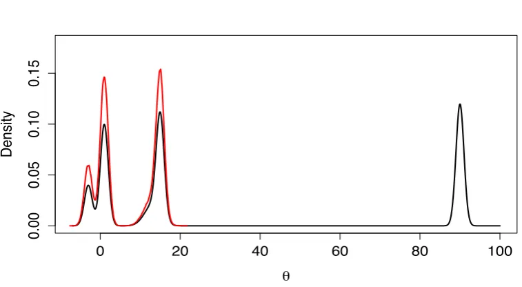
Consider using the MH algorithm to target a distribution, π, that is multi-modal with the modes being well separated; Figures 1.1 and 1.2 illustrate two such

ex-amples. It is important that a chain explores the entire space so that the sample estimates are unbiased thus validating Monte Carlo integral approximations of the

form (1.4). Typically the proposal mechanisms used in MH algorithms are localised

and tuned to explore the local mode efficiently. However, this localisation essentially means that the Markov chain becomes trapped in a subset of the state space and

(even though it theoretically satisfies all ergodicity properties in the prior section)

in the finite run time it fails to explore all regions of significant probability mass. The resulting algorithm’s performance in the finite run can appear similar/identical

to one that fails to satisfy the irreducibility criteria introduced in Definition 1.2.3.

Figures 1.1 and 1.2 show an example where a Gaussian random walk on a toy multi-modal target for only a finite number of runs of the algorithm could result in

the algorithm only exploring a restricted subset of the support of the distribution.

(20)

optimal 0.234, Robertset al. [1997], the Markov chain entirely fails to explore the

full target distribution.

0 20 40 60 80 100

0.00

0.05

0.10

0.15

θ

[image:20.595.123.502.162.370.2]

Density

Figure 1.1: One dimensional target density (black) constructed from a Gaussian mixture distribution, over-plotted (in red) with the kernel density estimate from a 1000000 run RWM (tuned to give an approximately 0.234 acceptance rate).

Indeed many of the most effective and scalable proposal mechanisms for MH

utilise the local gradient information with the Metropolis Adjusted Langevin Al-gorithm (MALA), e.g. Roberts and Stramer [2002], and Hamiltonian Monte Carlo

(HMC), e.g. Girolami and Calderhead [2011], being arguably the most famous meth-ods. Essentially, this class of techniques use local gradient based information that

“directs” the proposed move uphill to regions of higher density. This is a

heuris-tically sensible approach when the target is uni-modal; however, when the target distribution is multi-modal with insignificant bridging mass, then these methods

tend to make the problem even worse since the gradient information helps to draw

the Markov chain back towards the local mode.

In cases where the modes are “close” then approaches that incorporate

am-bitious proposals, e.g. Green and Mira [2001], could be used. Also, if one knows the

locations of modes beforehand, then a carefully designed mixture proposal would allow for inter-modal jumps. In general, the form of the target isn’t known, and if

naive algorithms tuned to localised exploration are used the user will be unaware

(21)

Figure 1.2: Left: 2D Gaussian mixture target density (black). Right: over-plotted (in red) with the sample of a 1000000 run RWM (tuned to give a 0.234 acceptance rate).

This motivates using a more advanced MCMC algorithm to sample from

the target distribution in cases which exhibit multi-modality. The major problem is

that the regions of significant probability mass do not have significant bridging mass that allows the chains to traverse along to get from region to region using localised

moves. Using proposals like the Gaussian increments in RWM with large ambitious

scalings in the hope the proposal will land in another modal region inevitably has extremely low acceptance rates and performance tends to deteriorate dreadfully in

higher dimensions.

Definition 1.3.1(Tempered Target at Inverse Temperatureβ). For a target distri-butionπ(·), the tempered target at inverse temperatureβ, denotedπβ(·), is defined

as

πβ(x)∝π(x)β

forβ∈(0,∞); and it is only a proper distribution providedR

Xπ(x)βdx <∞.

Such distributions are useful for a range ofβ values, including for

optimisa-tion problems in the simulated annealing framework where one considers β → ∞

with an invariant Markov chain (hopefully) becoming trapped in the mode with

the global maximum, Kirkpatrick et al. [1983]. For the purposes of sampling from

(22)

β∈(0,1].

Asβ →0 then πβ(·) approaches a (potentially improper) uniform

distribu-tion on the support of the target distribudistribu-tion. Essentially, this has the effect of

flattening out the target distribution by spreading out mass into the tails of the

distribution and forming bridging mass between modes. Herein, tempered targets raised to a powerβ ∈(0,1) will be will be described as hot state target distributions. This nomenclature emanates from the physics literature where,π(x)∝exp{−H(x)}

with −H(x) < 0 being the potential, so by heating the system to a temperature T = 1/β (hence multiplying the potential byβ) this increases the energy in the

sys-tem. As such the cold state will be used herein to describe the target distribution

with no heating (i.e. β= 1).

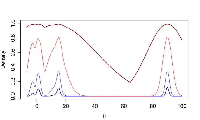
Figure 1.3 illustrates the effect of tempering on the target density used in

Figure 1.1 and shows that the (normalised) tempered densities appear to approach

an improper uniform distribution and have crucially provide bridging mass between the modes.

0 20 40 60 80 100

0.00

0.04

0.08

0.12

θ

Density

Figure 1.3: Tempered densities for β={1,0.5 ,0.1,0.005}, corresponding to (dark blue), (light blue), (red) and (dark red) respectively.

The tempered distributions have the same support and also have their modes

in the same locations as the untempered distribution (since powering is a monotone

function). As such, for a suitably hot temperature level target, basic methods such as RWM or HMC should be able to efficiently explore the space. Using these hot

(23)

from the mixing ability in the hotter state tempered distributions to enable full

exploration of the state space in the cold level target state.

Two fundamental and widely used algorithms that exploit these tempered

targets to aid mixing in multi-modal settings are the parallel and simulated

tem-pering algorithms; these are introduced in the following Section 1.4, along with alternative and rivaling approaches for multi-modal settings.

1.4 Algorithms for Multi-Modal Target Distributions

Section 1.3 motivated the use of advanced algorithms for sampling from a

multi-modal distribution. Under a given parametrisation, the target distribution is fixed

and so the performance of an MCMC algorithm depends upon the proposal mech-anism employed. Section 1.3 suggested that mixing information from the chains

targeting the hotter, tempered distributions could be used to aid inter-modal

mix-ing at the target cold state. Geyer [1991] and Marinari and Parisi [1992] introduced the Simulated tempering (ST) and Parallel tempering (PT) algorithms to do this. In

this section the ST algorithm will be introduced and its major drawback highlighted,

motivating the more practically favoured PT algorithm.

After this a brief review of alternative/competing algorithms that attempt

to overcome the issues of multi-modality will be explored.

1.4.1 Simulated Tempering (ST) Algorithm

Consider a sequence ofd-dimensional tempered target distributions (on a state space

X) defined at inverse temperature levels{β0, . . . , βn} where 0≤βn< βn−1 < . . . <

β1< β0 = 1. The simulated tempering approach introduced by Marinari and Parisi

[1992], runs a single (d+ 1)-dimensional Markov chain, (β, X), on the extended

extended state space {β0, . . . , βn} × X, cycling between moves within the current

temperature level and temperature level swap moves to mix through the temperature schedule. The invariant distribution of the chain, (β, X), defined on the extended

state space{β0, . . . , βn} × X is

π(β, x)∝K(β)π(x)β (1.9)

where ideally (but unrealistically) K(β) = R

xπ(x) β_dx−1

, resulting in each

(24)

Simulated Tempering (ST) Algorithm:

• Choose a sequence of tempering values 0≤βn< βn−1 < . . . < β1 < β0= 1.

• Choose initial values of the chainβ0 and x0.

• Choose the proposal mechanisms for all within temperature level type moves, denotedqβj(y|x) for j= 0,1, . . . , n.

• Choose the number, m, of within temperature proposals the chains will per-form before attempting a swap type move and choose the total number,s, of

swap moves that will be attempted.

• Iteratestimes:

1. If currently in temperature levelβj uniformly randomly propose to move

to one of the adjacent temperature levels,β0 ∈ {βj−1, βj+1}say. (Denote

the current position of the chain in theX space as x).

2. Compute the acceptance ratio for the proposed move (βj → β 0

) and

accept the move with probability equal to

min 1,K(β

0

)π(x)β

0

K(βj)π(x)βj

!

. (1.10)

3. Perform m within temperature moves to target the current inverse

tem-perature level target using the proposal mechanism specified for the

cur-rent inverse temperature value.

ChoosingK(β) to normalise the marginal temperature levels is not necessary for the running of the algorithm; indeed knowing the normalisation constants apriori

is highly unlikely for most problems of interest. Figure 1.4 illustrates an example

of un-normalised tempered targets when the convenient choice ofK(β)∝1 is used. The key problem with not having marginally normalised targets is highlighted by

considering the marginal distribution of the inverse temperature values. Assuming

K(β)∝1, then by integrating out x from the joint distribution,

π(β)∝

Z

X

π(β, x)dx=K(β)

Z

x

π(x)βdx (1.11)

and so π(β) ∝R

xπ(x)

β_{dx. Thus the chain can end up spending dramatically}

(25)

0 20 40 60 80 100

0.0

0.2

0.4

0.6

0.8

1.0

θ

[image:25.595.150.493.108.313.2]

Density

Figure 1.4: Tempered Densities for β={1,0.5,0.1,0.005}, corresponding to (dark blue), (light blue), (red) and (dark red) respectively with normalising constants

K(1) = 1, K(0.5) = 0.21,K(0.1) = 0.04, K(0.005) = 0.009.

higher dimensionality. Indeed, this is an issue explored by Wang and Landau [2001] and later (and specifically for a general state space simulated tempering algorithm)

Atchad´e and Liu [2004]. Also, importance sampling, or more specifically,

meth-ods such as bridge sampling, Meng and Schilling [2002], can be used to attempt to approximate normalisation constants but this is a non-trivial task in multi-modal

settings.

As a concrete example of the dangers of using un-normalised marginals for the simulated tempering algorithm consider Figure 1.3 with normalised tempered

densities for a Gaussian mixture target distribution and the contrastingly powered

up but un-normalised versions in Figure 1.4. Numerical integration allow us to compute the marginal distribution of the β’s: π(β = 0.005) = 0.77, π(β = 0.1) =

0.19, π(β = 0.5) = 0.03,π(β = 1) = 0.007. Even in this single dimensional setting

the Markov chain on the augmented state space would spend less that 0.7% of its time exploring the target cold state.

Example of the ST algorithm:

To demonstrate the utility of the simulated tempering algorithm, the toy problems

from Figures 1.1 and 1.2 are revisited. Recall, the respective chains were unable

(26)

a suitably constructed ST algorithm with a simple three level geometric schedule,

{1,0.05,0.052}, (and using importance sampling to normalise the marginals), the resulting Markov chain successfully explores all modes in the target distribution as

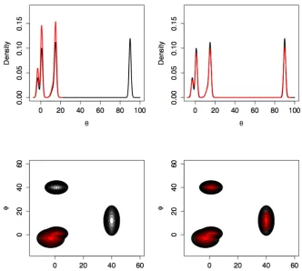
[image:26.595.147.480.200.498.2]

can be seen in Figure 1.5.

Figure 1.5: Top plots: are for the 1-dimensional example from Figure 1.1 and show the target density (black) and kernel density estimates (red) for the failure case using RWM (left) and the successful case using the ST algorithm (right). Bottom plots: are for the 2-dimensional example from Figure 1.2 with target density (black) and over plotted sample points (red), again for the failure case using RWM (left) and the successful case using the ST algorithm (right).

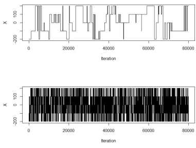
A convincing plot, in Figure 1.6, for the 1-dimensional example in Figure 1.5,

shows that it is indeed the auxiliary hot states mixing that is allowing effective

inter-modal mixing. Figure 1.6 shows the trace plot for the simulated tempering algorithm for the moves between 22000 and 24000 iterations. The background colour indicates

the temperature that the chain is at, with dark red being the hottest state and blue

(27)

key modal areas of density in the cold state are occurring due to the mixing of the

chain in the hotter states, with this mixing information then being fed back to the cold state.

Figure 1.6: Trace plot of a simulated tempering chain targeting the 1 dimensional distribution from Figure 1.1. The inverse temperature schedule is a simple 3 level geometric schedule,{1,0.05,0.052}and the respective temperature at each iteration is indicated by the background colour, with dark red being the hottest (0.052), pink the intermediate temperature (0.05) and blue the target cold state. This highlights how the chain is only able to traverse between areas of significant mass when in the hottest states.

1.4.2 Parallel Tempering (PT) Algorithm

The major practical drawback of using the ST algorithm is with regards to the

lack of normalised marginals at each of the temperature levels. In toy or simple

low dimensional examples numerical integration or well designed importance sam-pling methods could be used, although this essentially defeats the need to then use

MCMC. In high dimensional, complex settings this isn’t feasible.

Consider running,n, Markov chains in parallel with one at each of the differ-ent temperature levels that the previously considered ST algorithm could have used,

(28)

For this augmented state space,Xn_{, the limiting target distribution is defined to be}

πn(x0, x1, . . . , xn)∝πβ0(x0)πβ1(x1). . . πβn(xn).

The chains running at the hotter temperatures have the improved fast mixing

and the aim is to pass this mixing information to the cold state target chain. One

approach is to propose a swap move between two chains in tandem; essentially proposing a jump in each chain to the location of the chain at the other (typically

consecutive) temperature level.

Suppose a swap type move is proposed between inverse temperature levels βj and βk. To ensure that this swap move preserves invariance it will be accepted

based on the usual Metropolis-Hastings acceptance probability,

min 1,πβj(xk)πβk(xj) πβj(xj)πβk(xk)

!

. (1.12)

Hence using this setup gives the same benefits as ST with the auxiliary hot

state mixing information aiding the inter-modal mixing in the cold states. However,

it is clear from equation (1.12) that the swap acceptance probability no longer depends on any marginal temperature normalisation constants since they all cancel

in the ratio.

Although, very close to the ST procedure with obvious tweaking, the PT procedure is now given and it will be referred to throughout the remainder of the

thesis with the shorthand notation PT:

Parallel Tempering (PT) Algorithm:

• Choose a sequence of tempering values 0≤βn< βn−1 < . . . < β1 < β0= 1.

• Choose initial values of the chains for each temperature level,x0₀, x0₁, . . . , x0_n.

• Choose the proposal mechanisms for all within temperature level type moves, denotedqβj(y|x) for j= 0,1, . . . , n.

• Choose the number, m, of within temperature proposals the chains will per-form before attempting a swap type move and choose the total number,s, of swap moves that will be attempted.

(29)

1. Uniformly randomly select a pair of adjacent temperatures, 1/βj and

1/βj+1 say, for which a swap move is proposed, and where the values of

the respective chains are (currently)xj and xj+1.

2. Compute the acceptance ratio for the proposed swap and accept the swap

with probability equal to

min 1,π(xj)

βj+1_π(x j+1)βj

π(xj)βjπ(xj+1)βj+1

!

. (1.13)

3. Perform m within temperature moves for each of the (n+ 1) chains

ac-cording to their respectively specified proposal mechanisms.

Note that in this setup only swap moves between consecutive temperatures is

con-sidered. The reason for this will be apparent from the discussion on optimal tuning

for the PT algorithm discussed in Section 1.5. Also note the significant opportunity to parallelise this approach so that then chains don’t require n times longer

run-time; indeed, VanDerwerken and Schmidler [2013] note substantial computational

gains can be made for the PT algorithm.

1.4.3 Associated and Rival MCMC Algorithms for Multi-modality

For completeness, this section discusses some of the notable and associated

algo-rithms used in an MCMC framework that are either closely linked to the ST and

PT algorithms or have rivaling approaches altogether.

• The Equi-Energy Sampler, Kouet al.[2006], Andrieuet al.[2007], is an ap-proach very similar to the PT algorithm. Suppose that the target distribution

has the form π(x) ∝ exp{−h(x)} where h(x) denotes the energy. Then sup-pose a sequence of energy bands are created (potentially adaptively through the run of the algorithm Schrecket al. [2013]) withH0 < H1. . . < Hn+1 =∞

withH0 <infx∈Xh(x), hence partitioning the energy space.

The basic idea is that multiple chains are run on a sequence ofn (truncated)

tempered target distributions with theithgiven byπi(x)∝exp{−h(x)∨Hi}.

The samples generated at each level are grouped into the (typically predefined) energy bands partitioned by the Hi’s. The process begins by only sampling

from the π0(·) distribution. After some burn-in period, sampling from π1(·)

(30)

continues, sequentially adding new levels until the target state is reached at

πn+1(·).

The “swap moves” between target levels are proposed and accepted with the

same MH ratio as in the PT approach. The major difference is that the swap location from the hotter temperature level are selected uniformly from

all historical locations of the hotter chain that share the same energy band

indicator as the cooler chain; thus inducing high acceptance rates of the swap proposals.

• Tempered Transitions: Neal [1996] introduced the tempered transitions approach to sampling from a multi-modal target distribution in an MCMC

framework. Like the ST and PT algorithms this method still utilises tempered target distributions. However, unlike the PT and ST algorithms, the core

Markov chain requires no state-space augmentation but instead the tempered

targets are interwoven into the proposal mechanism. Essentially, the proposal is made up from a sequence of proposals that create a path through the chosen

sequence of tempered target levels to the hottest state and then back to the

cold target state by which point the hope is that the final position is in a different mode. As will be seen, the number of temperature levels required in

high dimensional tempering procedures depends on the dimension and so the

proposal complexity can scale quite badly with dimension and indeed without very carefully constructed paths, the acceptance of these moves deteriorates

with dimension making the method difficult to tune.

• Mode Jumping Proposals: Tjelmeland and Hegstad [2001] designs an algo-rithm that uses optimisation techniques to find a localised mode upon proposal of a large initial proposal away from the current mode; then proposing from an

appropriate Gaussian distribution from the mode point. Indeed this has some

interesting links with the work in Chapter 4, specifically Section 4.3.4, where optimisation methods are used. Both Al-Awadhi et al. [2004] and Jennison

and Sharp [2006] consider similar approaches, with the former more generally

for a Reversible Jump MCMC framework, and essentially use a sequence of localised MH moves to be made after an ambitious initial move has been

pro-posed in the hope that the ensuing localised moves will drift towards the mode

point. Behrens [2008] takes a slightly different approach by doing a prior scan of the statespace for modes using a series of parallel, optimising, simulated

annealing procedures designed to locate modes and then using e.g mode point

(31)

a standard proposal during the MH scheme. This has the nice feature that

the actual run of the algorithm is relatively cheap but setup costs are high, and the mixture approximation’s accuracy can be an issue resulting in low

acceptance rates. A criticism of any scheme relying on locating modes prior

to the run of the algorithm is that such approaches tend to leave no ability to adapt if modes are missed initially or if the fitted mixture proposal is poorly

fitted.

• A Repulsive-Attractive Metropolis Algorithm for Multimodality:

Tak et al. [2016] introduce another very interesting idea where the proposal mechanism, similar to the tempered transitions approach, is constructed from

a sequence of proposals. Only localised MH moves are made but for the first

stage of the sequence of moves that make up the proposal trajectory, the in-verse of the target distributionπ is targeted, creating a repulsion effect away

from the local mode and (hopefully) then attracted towards a different mode

on the latter part of the trajectory. Only a single chain is needed, but like the tempered transitions approach, it is difficult to tune the number of steps in

the path of the proposal especially in high dimensional complex settings.

• Nemethet al.[2017] introduce an ingenious approach that augments the state space in a way that permits a target distribution with direct bridging mass between modes. Ultimately this allows the fast mixing HMC algorithm to

sample from this target by moving along the contours of the extended target

density. This approach requires a computational cost which could become large since the method requires N “temperature levels” similar to the PT

approach but then for the running of the HMC algorithm then augmentation

to 2N variables is required.

• Importance Sampling and SMC: Additionally, and beyond the scope of this review, there’s a vast range of competing approaches from the Importance

Sampling and Sequential Monte Carlo (SMC) literature e.g. Neal [2001]. A nice

idea that is closely linked to the PT approach is in Gramacyet al.[2010], where the issue of “wasted” samples in the PT algorithm arising from the augmented

levels is addressed. Gramacyet al. [2010] proposes using these as importance

samples for the cold target state and explores the optimal weighting strategy.

This thesis focuses on the development of two novel improvements to the PT algorithm. The new methodology is designed to overcome core issues that hinder

(32)

competing methods noted above suffer from the the problems noted in Chapter 4,

and almost all the methods noted above suffer from the issues targeted in Chapter 2. Hence, the thesis, albeit entirely focused on the PT approach, is in many senses

more broadly applicable to methodological improvement for many of the alternative

multi-modal solutions.

1.5 Optimal Setup of the Temperature Schedule

In both the ST and PT algorithms, a sequence of n+ 1 inverse temperature levels were required, {β0, . . . , βn}. Little was explained about why a schedule with

inter-mediate levels, rather than simply 2 levels (a hot level and cold level) are needed.

Clearly, once a sufficiently hot level has been chosen then the corresponding chain can mix through all areas of significant probability mass. Recall the acceptance

probabilities for the ST and PT algorithms respectively (1.10) and (1.12); these

preserve the invariance toπ and if one considers the hotter state chain as providing a proposal for the next location of the colder state chain then proposals to locations

that are unlikely under the target distribution are unlikely to be accepted.

As a heuristic, consider a one dimensional target distribution π which is a standard Gaussian distribution, i.e.

π(x)∝exp

−x

2

and so at inverse temperature levelβ

πβ(x)∝exp

−βx

2

hence the target distribution is still Gaussian but with variance 1/β. Figure 1.7 shows the normalised density of π(x) but is over-plotted by the (also normalised)

target density at inverse temperature level β = 0.1. Clearly, locations for samples

from the hotter target are very likely to occur in areas that are unrepresentative of the cold state target and hence one would expect that temperature swap move

proposals from these locations would be rejected.

The bigger the gap in the temperature space between consecutive levels the larger that this issue becomes and as the gap increases the acceptance rate of swap

moves between these levels diminishes to zero. Consequently, a schedule with inter-mediate temperatures is used to feed the mixing information from these hot states

(33)

Figure 1.7: Black line: density of a standard Gaussian distribution. Red line: density of a standard Gaussian at inverse temperature level β = 0.1. Note the limited overlap of representative sample locations between the two densities.

The setup of these temperature levels is a fundamental issue to the

algo-rithm’s performance. Just like tuning the scaling of the variance when using RWM, Robertset al. [1997], there is a “Goldilocks” principle.

• Making the spacings too large results in low acceptance rates and slow mixing through the temperature schedule.

• Making the spacings too small means that there are many intermediate levels to mix through on the temperature schedule to get from the hot state to the cold state; again leading to slow mixing through the temperature schedule.

This issue becomes increasingly problematic with an increase in

dimensional-ity of the problem. To emphasise this consider ad-dimensional target distributionπ

which is constructed fromdiid standard Gaussian marginals. The swap acceptance probability for a temperature swap move between inverse temperaturesβ and β0 in

a PT setup wherey∼π_β0 and x∼π_β is

min

(

1,exp −β

0

−β 2

d

X

i=1

x2_i −y2_i

!)

(1.14)

but as d→ ∞ then by the law of large numbersPd

i=1x2i → dEβ(X2) =d/β and

similarlyPd

i=1yi2 → dEβ0(Y2) = d/β 0

(34)

given by

min



 

 

1,exp



 −

β0−β

2

2ββ0 d



 



 

 

. (1.15)

The acceptance ratio is then clearly exponentially decreasing in dimension.

Conse-quently, for a fixed spacing=β0−β, the acceptance probability of a swap between consecutive temperatures will degenerate to 0 in the limit asd→ ∞. If the spacing here was scaled according to the dimensionality so that∝O(d−1/2_{), then the swap}

move acceptance probability in (1.15) stabilises to have a non degenerate limit as

d→ ∞.

This dimensionality degradation and ambition of proposal trade-off motivates

seeking a temperature schedule that has spacings that induce an “optimal” mixing

through the temperature space.

1.5.1 Existing Optimal Scaling for Temperature Spacings Results

Atchad´eet al.[2011] investigate the problem of selecting temperature spacings when

the dimensionality, d, of the target distribution tends towards infinity. Suppose

a swap move between two consecutive temperature levels, β and β0 = β + is proposed. To optimise the ambition of the consecutive spacings, a heuristically

sensible approach is to maximise (with respect to ) the ESJ D (see Section 1.2 and Definition 1.2.4) through the inverse temperature space. This is the approach

of Atchad´e et al. [2011] and their specific form ofESJ D through the temperature

schedule will be denoted herein byESJ Dβ

ESJ Dβ =Eπ

(γ−β)2

(1.16)

where γ = β + for some > 0 if the proposed swap is accepted and γ = β

otherwise. The expectation is taken with respect toπ, i.e. assuming invariance has been reached. Note thatESJ Dβ will be used as the target metric for optimality in

both Theorems 3.2.1 and 5.1.1 later on in this thesis.

Indeed, for the PT algorithm,

ESJ Dβ = Eπ

(γ−β)2

= 2×_E_π

P(Swap accepted)

= 2×Eπ

"

min 1,π(xj)

βk_π(x k)βj

π(xj)βjπ(xk)βk

!#

(35)

It is worth noting for those familiar with scaling arguments that the second equality

here is usually non-trivial and needs justification; in this case, with the discrete and one-dimensional nature of the temperature schedule this equality is trivial.

For tractability of optimisation, Atchad´e et al. [2011] restrict to the set of

d-dimensional target distributions with (iid) form:

π(x)∝

d

Y

i=1

f(xi). (1.18)

Furthermore, motivated by (1.15), for non degeneracy of the limiting behaviour of

theESJ Dβ as d→ ∞then the spacing, , between consecutive levels must have a

form

= `

d1/2. (1.19)

with`a positive constant to be chosen to attain an optimalESJ Dβ. Pursuit of the

optimal`, denoted ˆ`, leads to Theorem 1 of Atchad´e et al.[2011]:

Theorem 1.5.1. For the parallel tempering algorithm, under the above setting of (1.18) and (1.19), then as d → ∞ the ESJ Dβ is maximised when ` is chosen to

maximise

`2×2Φ −`

r

I(β)

2

!

where I(β) = V ar_πβ f(x)

. This optimal choice of ` corresponds to an acceptance rate of swap moves of 0.234 (3 d.p.). The maximised asymptotic ESJD is given by:

ESJDβ = (2/dI(β))×ACC×[Φ−1(ACC/2)]2. (1.20)

Using an almost identical proof, Atchad´e et al. [2011] showed an equivalent

result for the marginally normalised ST approach, where the ESJ Dβ then has the

slightly different form of

ESJ Dβ =2×Eπ

"

min 1,K(β+)π(x)

β+

K(β)π(x)β

!#

=:2×ACC. (1.21)

The result of which is given in Theorem 2 of Atchad´e et al. [2011] (given here).

Theorem 1.5.2. For the simulated tempering algorithm, under the above setting of (1.18), (1.19) and (1.21), then as d → ∞ the ESJ Dβ is maximised when ` is

chosen to maximise

`2×2Φ −`

p

I(β)

2

(36)

where I(β) = V ar_πβ f(x)

. This optimal choice of ` corresponds to an acceptance

rate of swap moves of 0.234 (3 d.p.). The maximised asymptotic ESJD is given by:

ESJ Dβ = (4/dI(β))×ACC×[Φ−1(ACC/2)]2. (1.22)

Insight and Impact of Theorems 1.5.1 and 1.5.2:

Theorems 1.5.1 and 1.5.2 give explicit formulas for derivation of the optimal `for consecutive temperature spacings. Albeit derived for target distributions that

are assumed to have iid type construction in (1.18), for a practitioner, the associated

0.234 optimal swap acceptance rate gives powerful setup guidelines. The theorems also suggest a strategy for optimal setup starting with a chain at the hottest level

and tuning the spacing to successively colder temperature levels based on the swap

acceptance rate to attain consecutive swap rates close to 0.234. Indeed, using a stochastic approximation algorithm, see Robbins and Monro [1951], then

Miasoje-dow et al. [2013] take an adaptive MCMC approach (see Roberts and Rosenthal

[2009]) to the setup of the temperature spacings with the target being to exploit the above 0.234 tuning suggested by Atchad´e et al. [2011].

In practice, for most interesting problems, the target will not satisfy the iid

assumption (1.18). Atchad´e et al. [2011] consider using the 0.234 rule when tar-geting an inhomogeneous Gaussian distribution and the Ising model, with neither

example satisfying the distributional assumption in (1.18). The first of these

ex-amples illustrates that even when the distribution doesn’t satisfy equation (1.18) the 0.234 rule still appears optimal when considering the empirical ESJ Dβ over

different spacings.

A highly insightful example is for the Ising model. Atchad´e et al. [2011]

compares the efficiency between an implementation of the 0.234 rule versus a

tradi-tionally chosen method of geometric spacing for the Ising model. The Ising model exhibits a phase transition (which is when there is a dramatic change in form of the

distribution) as the temperature reaches some hot critical value. Using the

tradi-tional geometric schedule, the parallel tempering algorithm performs poorly close to this temperature. However, Atchad´e et al. [2011] use the 0.234 rule which

al-locates a cluster of temperature levels around the critical temperature making it

easier for the temperature swaps to “bridge” this critical temperature level (due to the temperature level move being less ambitious).

Theorems 1.5.1 and 1.5.2 give insight between the relative efficiencies of the

(37)

in equation (1.20) is half that for theESJ Dβ of the ST procedure given in

equa-tion (1.21). Also, Atchad´e et al. [2011] show that the optimal spacings between inverse temperature levels are √2 times larger for ST than for PT. This implies that compared to the PT scheme, the ST procedure is twice as efficient at mixing

across the temperature space. This suggests preference towards the simulated tem-pering scheme. However, the optimal ESJ Dβ was computed for the ST algorithm

assuming the marginal normalisation constants can be found (whereas the

normal-ising constants aren’t needed for parallel tempering). Furthermore, the temperature swap in a PT scheme aids the mixing for two chains simultaneously whereas with

ST mixing is only for a single chain.

Recall that in Section 1.2 the use ofESJ Dwas justified under the assumption that there is an associated limiting diffusion process. Atchad´e et al.[2011] used the

ESJ D but noted that full justification requires proof of existence of a limiting

diffusion process. This was subsequently studied in Roberts and Rosenthal [2014]. Initially and crucially Roberts and Rosenthal [2014] establish that for two

non-explosive diffusion processesXσ1 _and _Xσ2 _{with the same invariant distribution,}_π,

and where σ1(·) and σ2(·) are the variance functions, then ifσ1(x) > σ2(x) for all

pointsxin the state space thenXσ1 _{is more efficient with respect to the asymptotic}

variance of estimates ofL2(π) functionals i.e. forf ∈L2(π)

lim

T→∞ T

−1/2 _Var

Z T

0

f(Xσ1 s ) ds

!

≤ lim

T→∞ T

−1/2 _Var

Z T

0

f(Xσ2 s ) ds

!

.

Roberts and Rosenthal [2014] compute the diffusion limit of the inverse

tempera-ture component, i.e. β, of an ST procedure under the same assumptions on the scaling and target form as Atchad´e et al. [2011]. This gives a functional form of

the diffusion volatility as a function of `, i.e. σ`(β). This can be maximised with

respect to` at the fixed inverse temperature levelβ to give ˆ`(β), ensuring optimal asymptotic efficiency. Reassuringly, Roberts and Rosenthal [2014] concluded that

optimal spacings are identical to those considered optimal in Atchad´e et al. [2011]

and have a corresponding expected acceptance rate of 0.234 between consecutive temperature levels.

1.5.2 The Relationship with Geometric Spacings

The problem of choosing optimal spacings has been studied previously in the physics

(38)

between swap moves (in agreement with the scaling theorems of Atchad´e et al.

[2011]). However, in both cases this is found for distribution functions with far more restrictive forms than that of equation (1.18).

A major observation of Atchad´eet al.[2011] is that temperature levels should

be setup consecutively. Previous studies and practitioners typically used a geometric inverse temperature schedule.

Definition 1.5.1 (Geometric Temperature Schedule). A geometric (inverse) temperature schedule refers to a temperature schedule setup with inverse tem-peratures given by 1 =β0 > β1 > . . . > βn>0 where for a fixed constantC ∈(0,1)

βi+1 =Cβi.

Atchad´eet al.[2011] show that, under their setting, the optimal temperature schedule will only be geometrically derived ifI(β) = Var_fβ(logf)∝1/β2.

To see this, consider the optimal scaling PT result in Theorem 1.5.1 and note

that the limitingESJ Dβ is given by

`2

d ×2Φ −`

r

I(β)

2

!

.

Substituting inu=`pI(β) and then maximising now with respect tougives a value

ˆ

u (which importantly doesn’t depend on I(β)). Then the corresponding optimal ` is given by

ˆ

`= _puˆ

I(β).

Now for a geometric schedule then ˆ` must be proportional to β with the

constant of proportionality not depending on the value ofβ. This happens ifI(β)∝

1/β2. A key example is for the setting of a uni-modal iid Gaussian target since in this case I(β) = 1/β2. This is the fundamental justification for the use of a geometric schedule for the canonical Gaussian empirical examples of Section 2.7,

and later on, this is used in the derivation of the result in Corollary 5.2.1.

1.6 Torpid and Rapid Mixing of the PT Algorithm

Atchad´e et al. [2011] and Roberts and Rosenthal [2014] give practical guidance to setup the temperature schedule in an optimal way. From the perspective of the

ST/PT algorithm, both Atchad´eet al.[2011] and Roberts and Rosenthal [2014], seek