Sequential stopping for high throughput experiments

(1)

http://wrap.warwick.ac.uk

Original citation:

Rossell, David and Muller, P.. (2013) Sequential stopping for high-throughput

experiments. Biostatistics, Volume 14 (Number 1). pp. 75-86. ISSN 1465-4644

Permanent WRAP url:

http://wrap.warwick.ac.uk/53407

Copyright and reuse:

The Warwick Research Archive Portal (WRAP) makes this work of researchers of the

University of Warwick available open access under the following conditions.

This article is made available under the Creative Commons Attribution 3.0 Unported (CC

BY 3.0) license and may be reused according to the conditions of the license. For more

details see:

http://creativecommons.org/licenses/by/3.0/

A note on versions:

The version presented in WRAP is the published version, or, version of record, and may

be cited as it appears here.

(2)

doi:10.1093/biostatistics/kxs026

Advance Access publication on August 20, 2012

Sequential stopping for high-throughput experiments

DAVID ROSSELL∗

Biostatistics and Bioinformatics Unit, Institute for Research in Biomedicine of Barcelona, Barcelona 08028, Spain

[email protected]

PETER M ¨ULLER

Department of Mathematics, UT Austin, Austin 78712, TX, USA

SUMMARY

In high-throughput experiments, the sample size is typically chosen informally. Most formal sample-size calculations depend critically on prior knowledge. We propose a sequential strategy that, by updat-ing knowledge when new data are available, depends less critically on prior assumptions. Experiments are stopped or continued based on the potential benefits in obtaining additional data. The underlying decision-theoretic framework guarantees the design to proceed in a coherent fashion. We propose intu-itively appealing, easy-to-implement utility functions. As in most sequential design problems, an exact solution is prohibitive. We propose a simulation-based approximation that uses decision boundaries. We apply the method to RNA-seq, microarray, and reverse-phase protein array studies and show its potential advantages. The approach has been added to the Bioconductor packagegaga.

Keywords: Decision theory; Forward simulation; High-throughput experiments; Multiple testing; Optimal design; Sample size; Sequential design.

1. INTRODUCTION

In high-throughput studies (HTSs), the sample size is usually chosen informally. The resulting exper-iment may either be not informative enough or unnecessarily extensive. To address this problem, we develop a sequential design framework for HTSs. That is, we investigate the question whether the currently available data in a typical HTS suffices and, if not, how to determine the optimal stop-ping strategy. We focus on experiments to perform group comparisons, although our ideas remain use-ful for other inferential goals. For simplicity, we discuss the two-group case, but our software allows

>2 groups. The proposal is based on Bayesian decision theory, so that decisions are coherent with respect to an underlying utility function and probability model. We emphasize ease of interpretation and use.

Several authors proposed fixed sample-size calculations for HTSs, i.e. the sample size is fixed at the beginning of the experiment (Dobbin and Simon,2007;Lee and Whitmore,2004;M¨ullerand others,

2004; Panand others,2002;Zienand others,2003). The main limitations are the lack of flexibility to

∗_{To whom correspondence should be addressed.}

c

The Author 2012. Published by Oxford University Press.

This is an Open Access article distributed under the terms of the Creative Commons Attribution License (http://creativecommons.org/licenses/by/3.0/), which permits unrestricted reuse, distribution, and reproduction in any medium, provided the original work is properly cited.

at University of Warwick on August 22, 2013

http://biostatistics.oxfordjournals.org/

(3)

incorporate new data and the need for a good prior guess of certain features, e.g. effect sizes or the pro-portion of differentially expressed (DE) genes.

In contrast, sequential sample-size designs update knowledge and make decisions as data are collected, i.e. they are robust with respect to prior choices. A sequential design stops or continues experimentation on the basis of all available data. A potential drawback is the need to carry out experimentation in batches. The associated increase in time or experimentation costs may outweigh the potential advantages. This should not be a major concern in many HTSs, as most high-throughput technologies (e.g. microarrays, sequencing, or mass spectrometry) process samples in small batches. Assessing the promise of continuing experimentation after each batch seems natural. Also, samples may be costly to obtain or there may be ethical concerns, e.g. in human studies. These situations offer great potential for sequential strategies.

Ruppertand others(2007),Tibshirani(2006), andFerreira and Zwinderman(2006) proposed two-step designs focused on microarray differential expression problems. Two-step designs adapt to the observed data to a limited extent.Gibbonsand others(2005) andDurrieu and Briollais(2009) propose sequential designs that select a single/few genes and stop the trial when differences in expression can be estimated with high precision. The focus on a few genes limits the application to HTS. Researchers typically use HTS as a screening test to identify candidates, which are then validated with more precise techniques (e.g. real-time PCR). The usual goal is not to estimate differential expression accurately but to find promising targets. TheDurrieu and Briollais(2009) model is appropriate for paired observations, e.g. two-channel arrays.

We propose an approach for unpaired data that screens a large number of candidates and attempts to maximize the number of promising targets. The framework is directly applicable to many probability models and experiments, including sequencing, microarrays, and reverse-phase protein arrays (RPPAs). With minor modifications, it can be adapted to other experimental goals. The main hurdle with decision-theoretic optimal sequential designs is the prohibitive computational cost, even in single-outcome experi-ments.Rosselland others(2006) developed an approach based on the ideas ofM¨ullerand others(2006),

Brockwell and Kadane(2003), andCarlinand others(1998). They compute a summary statistic S each time new data are observed and they use decision boundaries that partition the sample space. The exper-iment is terminated whenS first falls in the stopping region. The sequential problem is reduced to the (non-sequential) problem of finding optimal boundaries. The choice of these boundaries accounts for all future data, which distinguishes the solution from myopic approximations. Here we extend these ideas to high-dimensional data and apply them to differential expression problems.

Section 2 formalizes the problem and two convenient probability models. Section 3 describes sequential stopping and the infeasibility of an exact solution. Section 4 proposes an approximate solution. Section 5 presents examples and Section 6 some concluding remarks. The supplementary material available at Bio-statisticsonline contains theoretical and practical considerations, and an example with the R code.

2. DATA FORMAT AND MODEL

We motivate the discussion in the context of experiments that study differential gene expression, but the proposal remains applicable to other setups. Letn be the number of outcomes (e.g. genes) andT be the maximum sample size.Tis usually determined by budget constraints, accrual rates, or an informed guess. Letxi j be the measurement for genei=1, . . . ,n and sample j=1, . . . ,T, andzj∈ {0, . . . ,nz}be the

group of samplej. For simplicity, here we assumezj∈ {0,1}, i.e. we compare two groups. Generalization

tonz>1 is straightforward and is implemented in thegagapackage.

A latent variableδi=1 indicates that geneiis DE across groups andδi=0 that it is equally expressed

(EE). The indicatorδirepresents the unknown truth and is part of the parameter vector. Letθi be

parame-ters indexing a probability model for(xi1, . . . ,xi T). Optionally, letωbe additional hyper-parameters. For

example,ωcould index a regression on important covariates. Letxt= {xi t,1in}be the data obtained

(4)

at timetandx1:t= {xi j,1in,1jt}be all data available up to timet. Further, letθ=(θ1, . . . ,θn)

andδ=(δ1, . . . , δn).

2.1 Probability model

Our proposal requires extensive predictive simulation and model fitting. Hence, the model must be com-putationally efficient. For instance, the examples in Section 5 required posterior inference in millions of simulated datasets. On the other hand, the model needs to be sufficiently flexible to capture the important features of the data.

Here we use the GaGa (Rossell,2009) and log-normal normal with generalized variance (NN) mod-els (Yuan and Kendziorski, 2006) models to illustrate the approach. Both offer a reasonable compro-mise between flexibility and computational cost. The GaGa model assumes xi j ∼Ga(αi, αi/λi zj). The

NN model usesxi j ∼N(μi zj, σ 2

i). The tripleθi=(λi0, λi1, αi)(GaGa) orθi=(μi0, μi1, σi2)(in the NN

model) incorporates gene-specific variability and gene-by-group specific means. A hierarchical prior on θi assigns positive prior probability to means being equal across groups. The GaGa hierarchical prior is

λ−1

i0 ∼Ga(α0, α0/ν), αi|β, μ∼Ga(β, β/μ),

λ−1

i1 |λi0, δi∼

Ga(α0, α0/ν) ifδi=1,

I(λi1=λi0) ifδi=0,

(2.1)

andP(δi=1)=π, independently acrossi. The hyper-parameters areω=(α0, ν, β, μ, π). The NN

hier-archical prior isμi0∼N(μ0, τ02),σ− 2

i ∼Ga(ν0/2, ν0σ02/2), also with probability of ties P(δi=1)=π,

independently acrossi. For this model,ω=(μ0, τ0, ν0, σ0, π). The GaGa sampling distribution for xi j

captures asymmetries that are frequently observed in HTS. The NN assumptions are similar to those of the popular limma approach (Smyth,2004), which has been found useful in many applications. The supple-mentary material available atBiostatisticsonline (Section 3) shows goodness-of-fit assessments that help choose the most appropriate model for a particular dataset.

In terms of computational complexity, conditional onωthe posterior distributions are available in closed form. We treatωas fixed, avoiding the need for Markov Chain Monte Carlo (MCMC) simulation. This substantially increases the computational speed. We estimateωvia expectation-maximization as inRossell

(2009) andYuan and Kendziorski(2006). The latter proposed a method of moments estimate for(ν0, σ02),

which can result in overestimatingπ. We illustrate this issue and outline a simple procedure to adjustπˆ in the supplementary material available atBiostatisticsonline (Section 4).

While we use these two models in our examples, the upcoming discussion of the optimal stopping policy remains valid for any alternative probability model.

2.2 Pre-processing

We assume that the data are suitably pre-processed. This is critical for meaningful inference. For instance, ignoring batch effects may bias or add uncertainty to group comparisons. We note that some technologies such as RNA-seq may be less sensitive to batch effects, and that these can be partially mitigated by good design, e.g. by balancing the number of samples in each group and batch. We recommend jointly pre-processing data after every batch, as some technical biases (e.g. probe or GC-content biases) may be better assessed once more data are collected.

Batch effects and other sources of variability may be either addressed in the pre-processing or in the analysis by including appropriate terms in the model. Following Yang and Speed (2002) and

Durrieu and Briollais (2009), we argue in favor of the former. As an illustration, letyi j be a vector of

(5)

covariates that are used in the adjustment, and assume that E(xi j|μi zj,yi j)=μi zj+g(yi j). Here, g(·)

captures the effect ofyi j on the outcome, and could represent a non-linear adjustment that cannot be

cap-tured by the analysis model. One could then use the partial residualsx˜i j=xi j − ˆg(yij)as the pre-processed data, wheregˆ(·)is an appropriate estimate ofg(·).

We note that the domain of the data must match the assumptions of the model. For example, while most technologies deliver positive expression measurements, pre-processed data may sometimes present negative values that are not allowed in the GaGa model. A simple strategy to deal with negative values is to definex˜i zj=xi zj +k, where the offsetk>0 ensures thatx˜i zj>0. Alternatively, definex˜i zj=e

x_{i z j}

, but this option may produce outliers that decrease the model goodness-of-fit. In practice, we recommend trying several transformations and producing some goodness-of-fit plots (e.g. see supplementary material available atBiostatisticsonline, Section 3).

3. OPTIMAL SEQUENTIAL STOPPING

3.1 Decision criterion

We formalize sequential sample-size calculation within a Bayesian decision-theoretic framework. The optimal design is chosen by maximizing the expectation of an appropriate utility function. At each deci-sion time, the expected utility is conditional on all available data (which may be no data at all) and averaged with respect to uncertainty on the model parameters and future data, assuming optimal future decisions.

It is convenient to distinguish sequential and terminal decisions. Sequential decisions correspond to stopping vs. continuation and are made after each batch of observations. Terminal decisions are the clas-sification of genes into EE (δi=0) or DE (δi=1), and are taken only upon stopping. Letst=s(x1:t)=1

indicate the sequential decision of stopping at timet and letst=0 indicate continuation. Equivalently,st

can be described by the stopping timeτ =min{t: st=1}. We usestandτinterchangeably. Letdi(x1:t)=1

(0) indicate the terminal decision to report genei as DE (EE). Also, letd(x1:t)=(d1(x1:t), . . . ,dn(x1:t)).

Bothst andd(x1:t)depend on all data available up to timet.

In a fully decision-theoretic approach sequential and terminal decisions are chosen to jointly maxi-mize the expected utility. Instead, we assume a fixed rule ford(x1:t)and focus on the optimal choice of

st only. We take terminal decisions using the Bayes rule ofM¨ullerand others(2004) to control the

pos-terior expected false discovery rate (FDR) below some specified level. The pospos-terior expected FDR is

(1/D)di(x1:t)[1−E(δi|x1:t)], whereD=

idi(x1:t)is the number of reported positives. We use the

0.05 level throughout.

Sequential stopping decisionsstare based on a utility function with sampling costcand a unit reward

for each correctly identified DE outcome

u(st=1,d(x1:τ),x1:τ,δ)= −cτ +

n

i=1

δidi(x1:τ). (3.1)

The second term in (3.1) is the number of true positives (TPs). The costcis the minimum number of TPs that make it worthwhile to obtain one more sample. This interpretation allows for easy elicitation ofc, without any reference to the formal mathematical framework. The utility function (3.1) focuses on statistical rather than biological significance, as the size of the effect is not considered. A simple alternative is obtained by substituting|μi1−μi2|δidi(x1:τ)in the summation in (3.1); seeM¨ullerand others(2004)

orRiceand others(2008) for other interesting alternatives. The upcoming discussion is independent of

the specified utility.

(6)

3.2 Optimal rule

The optimal stopping decisionstmaximizesu(·), in expectation over all unknowns, including parameters

(θ,δ), and future datax_τ₊1:T. An exact solution requires dynamic programming, also known as

back-ward induction (DeGroot,2004). At timet, the optimal decision is to stop if the posterior expected utility forst=1, denoted byu¯t(st=1,x1:t), is greater thanu¯t(st=0,x1:t). Evaluatingu¯t(st=1,x1:t)is usually

straightforward. For (3.1), we find

¯

ut(st=1,x1:t)= −ct+ n

i₌1

P(δi=1|x1:t)di(x1:t), (3.2)

where P(δi=1|x1:t)is the posterior probability that outcomeiis DE. The expectation is with respect to

δonly, as we fix the terminal decisiond(x1:t). The posterior probabilityP(δi=1|x1:t)can be computed

in closed form for some models (including GaGa and NN) or can easily be estimated from the MCMC output. Evaluatingu¯t(st=0,x1:t)is more challenging. An exact solution requires assessing the expected

utility for all possible future data trajectoriesxt+1, . . . ,xT, substituting the optimal decisionsst+1, . . . ,sT.

The computational cost is prohibitive.

4. APPROXIMATION BY OPTIMAL DECISION BOUNDARIES

Berryand others(2001),Brockwell and Kadane(2003),DeGroot(2004), andM¨ullerand others(2006) discuss alternatives to an exact optimal sequential solution. FollowingRosselland others(2006), we define sequential stopping boundaries. We restrict the maximization to rules that depend on the data x1:t only

through a summary statisticSt and linear boundaries that partition the sample space. We propose using

St=tU, where

tU≡Ext+1[u¯t+1(st+1=1,x1:t+1)|x1:t]− ¯ut(st=1,x1:t)−c

is the one-step ahead increase in the expected utility andExt+1(·|x1:t)conditions onx1:tand marginalizes

with respect to future dataxt+1. For (3.1), we findtU=t(TP)−c, i.e.tU is the expected increase

in the TPs, and decision boundaries can equivalently be written in terms oft(TP).

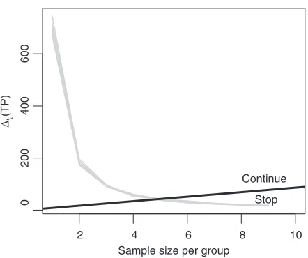
Consider the example in Figure1. The thick black line is a decision boundary. Every time we observe new data, we computet(TP). Ift(TP)lies above the boundary, we continue experimentation, otherwise

we stop. That is, we experiment as long as enough new TPs are expected.

Letb=(b0,b1)be the intercept and slope defining the linear boundaries, andU(b,x1:t)be the

associ-ated expected utility given data up to timet. In other words,U(b,x1:t)is the expected utility conditional

onx1:t when the stopping decision is based on a decision boundary indexed byb. Algorithm 1 details a

forward simulation algorithm (Carlinand others,1998) to evaluate the required expectations, and a grid search to carry out the maximization ofU(b,x1:t)with respect tob. The algorithm assumes thattsamples

are already available. For no data uset=0 andx1:t= ∅(see Section 5.3).

Algorithm 1. Optimal sequential boundary determination.

(1) Forward simulation. Simulatex(_t₊j)_1:_Tfrom the posterior predictiveP(xt+1:T|x1:t),j=1, . . . ,B. For

eachx(_kj), computet(TP)(j),k=t+1, . . . ,T.

(2) Grid search.For eachb, find the stopping timesτ(j)for all saved trajectoriest(TP)(j).

(3) Optimum. Selectb≡arg maxb{ ¯U(b,x1:t)}, whereU¯(b,x1:t)=(1/B)

B

j=1u¯(sτ(j)=1,x (j)

1:_τ(j)).

(7)

2 4 6 8 10

0

200

400

600

Sample size per group

Δt

(TP)

[image:7.536.159.380.71.256.2]

Stop Continue

Fig. 1. A GaGa model based optimal sequential boundary forc=50 (thick black line) and forward simulation trajec-tories (light gray lines), for example, in Section 5.1.

Figure1shows simulatedt(TP)as gray lines. For each boundaryb, we determine the stopping time

for each trajectory and average the expected terminal utilities. Att=T −1, we do not determine stopping usingbbut the optimal ruleT−1U>0.

In principle b can be recomputed every time new data are observed. Recomputation can help to decide between multiple optima and updateP(xt+1:T|x1:t). In our examples, we determinebonly once,

either based on a pilot dataset or prior knowledge, but we indicate the usefulness of recomputation when appropriate.

In addition to the intuitive appeal, some theoretical considerations motivate our approach. First, fixed-sample designs are special cases, e.g.b=c(4.5,∞)results in a fixed sample size of 5. The myopic rule of continuing as long astU>0 (Berry and Fristedt,1985, Chapter 7) is the special caseb=(c,0). We

generalize the idea with an arbitrary boundary ontU. An important assurance is thattTP converges

to 0 ast→ ∞, which guarantees eventual stopping; see supplementary material available atBiostatistics online (Section 1) for a formal statement and proof.

5. EXAMPLES

We compare our approach and the fixed sample designs ofM¨ullerand others (2004) in several impor-tant experimental conditions. The supplementary material available atBiostatistics online discuss pre-processing and goodness-of-fit (Section 3) and an additional RNA-seq example with the R code (Section 4).

5.1 Simulated microarray study

We plan collecting data in batches of 2 arrays per group, with a maximum of 20 per group (i.e.T=10 batches). Recall thatcis the minimum number of new DE genes that compensate the cost of one more batch. We considerc=25, 50, and 100. To keep the simulation realistic, we estimated the hyper-parameters based on data from a study of leukemia microarray data (Armstrongand others,2002). We focus on 24 acute lymphoblastic leukemia (ALL) and 18 mixed-lineage leukemia (MLL) trans-location samples. The

(8)

[image:8.536.82.455.105.234.2]

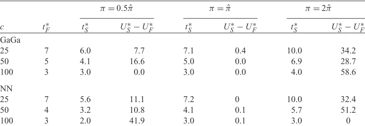
Table 1.Simulated data. tF∗:fixed sample size;t∗S:average sequential sample size;US∗−UF∗:

expected utility for sequential design minus the expected utility for a fixed sample

π=0.5πˆ π= ˆπ π=2πˆ

c t∗_F t∗_S U_S∗−U_F∗ t_S∗ U_S∗−U_F∗ t_S∗ U_S∗−U_F∗ GaGa

25 7 6.0 7.7 7.1 0.4 10.0 34.2

50 5 4.1 16.6 5.0 0.0 6.9 28.7

100 3 3.0 0.0 3.0 0.0 4.0 58.6

NN

25 7 5.6 11.1 7.2 0 10.0 32.4

50 4 3.2 10.8 4.1 0.1 5.7 51.2

100 3 2.0 41.9 3.0 0.1 3.0 0

estimated proportion of DE genes is πˆ=0.063 under the GaGa model and 0.05 for the NN model. We find optimal strategies based onπ= ˆπ, but we assess performance under model mis-specification by also simulating data underπ=0.5πˆ andπ=2πˆ, while leavingπ= ˆπ unchanged in the analysis model. We obtained 250 simulations under each scenario.

Figure1shows the optimal boundary forc=50 and simulatedt(TP)(gray lines) under the GaGa

model. Table1reports expected utilities and stopping times. The optimal fixed sample sizes forc=50 under the GaGa and NN models aret∗F=5 andtF∗=4, respectively. Whenπ= ˆπ, the expected

sequen-tial sample sizes are 5.0 and 4.1 (respectively) and there is no gain in the posterior expected utility. Sequential designs offer little advantages when the data match the prior expectations. However, when prior expectations are unrealistic, sequential designs adapt to the observed data. Whenπwas overstated by the prior (π=0.5πˆ), sequential designs stopped earlier than the fixed sample-size designs. Conversely, whenπ=2πˆ, they stopped later so that more DE genes could be found. For instance, forc=50 the GaGa sequential design requires 4.1 data batches whenπ=0.5πˆ and 6.9 whenπ=2πˆ. The fixed design always requires 5.

5.2 High-throughput sequencing example

We use a pilot RNA-seq dataset with two muscle and one brain human samples to design two hypothetical studies. Study 1 compares gene expression for muscle vs. brain. Many DE genes are expected. Hypothetical Study 2 compares the two muscle samples. No genes should be DE. In both cases, we use one sample per group as pilot data. We consider up to T=5 more samples, in batches of one sample. The GaGa model provided a reasonable fit to these data (supplementary material available at Biostatisticsonline, Section 3).

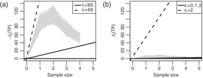
We determined the optimal boundary for sampling costs c=0,1, . . . ,100. Figure2(a) shows that

t(TP)is maximal fort=2 additional data batches. As suggested by Theorem 1 (supplementary

mate-rial available atBiostatisticsonline, Section 1), the incremental reward decreases ast grows further. The dashed boundary shows that, forc>66, the optimal decision is to stop experimentation. Forc66, there are multiple optimalb∗. The solid black lines show two optima. In both cases, the decision att=0 is to continue. Since the simulated trajectories do not cross either boundary, we expect experimentation to con-tinue up toT =5. The future realizedt(TP)might cross the boundary, in which case the design would

adapt and stop experimentation beforeT =5. Given that the pilot data contains one sample per group, we would re-determinebupon observing new data.

(9)

0 1 2 3 4 5

0

20

40

60

80

120

Sample size

Δt

(TP)

Δt

(TP)

c≤66 c>66

0 1 2 3 4 5

0

20

40

60

80

120

Sample size

c=0,1,2 c>2

[image:9.536.93.445.75.210.2]

(a)

(b)

Fig. 2. Simulated one-step expected increase in true discoveriest(TP)(gray lines) and optimal boundaries for several

sampling costsc(black lines). Left: brain vs. muscle (two multiple optimal boundaries shown forc66), right: muscle vs. muscle.

The hypothetical muscle vs. muscle comparison simulation is shown in Figure2(b). In this case,t(TP)

is negligible and the optimal design is to stop att=0 (i.e. not to collect any further data) for anyc>2. The result seems sensible as no DE genes are expected.

5.3 Microarray example

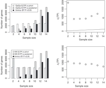
We consider the leukemia study ofCampo Dell’Ortoand others(2007) recording mRNA expression for 21 ALL and 15 MLL patients and 54 675 genes. We consider designing the study before any data were available. In such circumstances, one could estimate the hyper-parametersωfrom a similar study. We used theArmstrongand others(2002) study (Section 5.1) as it was also carried on ALL/MLL patients and used the same microarray platform. Once fixed and sequential designs were determined, we used the historical data to compare performance. We use batches of two arrays per group, maximumT=7 batches, andc=50. The white bars in Figure3(left panels) show the expected utility under the GaGa and the NN priors for all fixed sample sizes. The optimal fixed sample sizes aret∗F=5 batches (GaGa) andtF∗=4 (NN).

The right panels show the optimal boundaries andt(TP)computed from the observed data up to time

t=1, . . . ,7. For both models, the sequential design continues up to the time horizon. Figure3compares the designs by computing the posterior expected TPs (gray bars) and the number of genes with limma P-values<0.05 after theBenjamini and Yekutieli(2001) adjustment (black bars). At the time horizon both quantities increase over 2-fold compared with the recommended fixed sample size. The differences between prior and posterior expected TPs show how sequential designs adapt to the observed data to correct prior mis-specifications.

5.4 Reverse-phase protein arrays

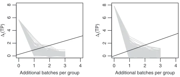
We design a follow-up study for the RPPA dataset dataIII that is included in the R package RPPanalyzer(Mannspergerand others,2010). The data contain expression for 75 proteins and 35 stage 2 and 25 stage 3 samples. Both models, the NN and GaGa models provide a reasonable fit (supplementary material available atBiostatisticsonline, Section 3). The fit under the NN model is slightly better. We find

π=0.13 under the NN model, andπ=0.10 under the GaGa model; that is, the estimated number of DE proteins is 9.75 and 7.5, respectively. Although we expect several DE proteins, at a posterior expected FDR

<0.05 the NN model calls one DE protein, and the GaGa model makes no DE calls. For comparison, only one protein has limma BY-adjustedP-values below 0.05.

(10)

2 4 6 8 10 12 14 Sample size

Number of genes

0

2000

4000

6000

8000

GaGa E(TP) a priori GaGa E(TP) a posteriori limma−BY P<0.05

2 4 6 8 10 12 14

0

500

1000

1500

2000

Sample size

Δt

(TP)

Δt

(TP)

2 4 6 8 10 12 14

Sample size

Number of genes

0

2000

4000

6000

8000

NN E(TP) a priori NN E(TP) a posteriori limma−BY P<0.05

2 4 6 8 10 12 14

0

500

1000

1500

2000

[image:10.536.96.443.79.367.2]

Sample size

Fig. 3. Sequential Analysis of Campo Dell’Orto’s data based on GaGa (top panels) and NN models (bottom panels). Left panels: expected number of TP (a priorianda posteriori) vs. sample size. Black bars indicate the number of genes with Benjanimi–Yekutieli-adjusted limmaP-values<0.05. Right panels:t(TP)vs. sample size and optimal

sequential boundary.t(TP)being above the boundary for alltindicates the experimentation continuing up to the

maximum sample size.

We consider adding batches of 50 samples per group, up to a maximum ofT =4. We set the sampling cost toc=1, reflecting that RPPA samples are relatively cheap. The study focuses on 75 carefully chosen proteins. Figure4shows simulatedt(TP)trajectories and the optimal boundaries. Inference under the

GaGa model estimates fewer TPs. Otherwise, inference is fairly similar across models and the optimal boundaries are remarkably close. The average sample size istS∗=1.37 under the NN model, andtS∗=1.32

under the GaGa model. The expected number of TPs attS∗is 9.46 (NN) and 6.11 (GaGa); that is, according

to both models, most DE proteins should be detected by adding 1–2 batches, i.e. 50–100 samples per group. These results help assess the potential benefits of extending the experiment.

6. DISCUSSION

We proposed a sequential strategy for massive multiple hypotheses testing. An important advantage lies in the generality of the proposed design. We discussed three RNA-seq, one microarray, and one RPPA experiments. Sequential designs are robust with respect inaccurate prior guesses and provide substantial advantages over fixed sample designs.

The proposal is formulated in a decision-theoretic framework and emphasizes interpretability. We moni-tor the one-step ahead expected increment in utility and stop the experiment when it falls below a boundary.

(11)

0 1 2 3 4

02468

Additional batches per group

Δt

(TP)

Δt

(TP)

0 1 2 3 4

0

2

4

6

8

[image:11.536.116.423.72.204.2]

Additional batches per group

Fig. 4. Simulatedt(TP)and optimal boundaries forc=1 in RPPA data using GaGa (left) and NN (right) models.

The approach includes fixed sample size and myopic designs as special cases. We use terminal decisions that control the posterior expected FDR. While inconsistent with a strict decision-theoretic setup, where all decisions are taken to maximize the expectation of a single utility, we feel that our choice offers a pragmatic compromise.

The method allows stopping when only one or two samples are available, which requires making strong parametric assumptions. For instance, in Figure3, the posterior expected TPs andt(TP)based on two

samples per group differ widely between the GaGa and NN models. Nevertheless, both models correctly indicate to continue and show good agreement for subsequent samples. Whenever possible, we recommend using a minimum burn-in (e.g.3 samples) before starting sequential stopping. When not feasible, we recommend assessing the goodness-of-fit carefully and updating the forward simulation when more data are available.

We focused on group comparison experiments, but the framework can serve as the basis for other HTSs. Interesting extensions include classification, clustering, or network discovery studies. These would require adjusting the utility function and possibly the probability model, e.g. to capture strong dependencies between outcomes.

Sequential designs are most appealing in moderate to large studies, where technical limitations require gathering data in batches. They should also prove valuable when samples are costly to obtain or there are ethical considerations, e.g. in human studies. Overall, they help save valuable resources and guarantee that sufficient data are collected to answer the scientific questions.

SOFTWARE

An implementation of the proposed approach was added to the Bioconductor package gaga.

SUPPLEMENTARY MATERIAL

Supplementary material is available athttp://biostatistics.oxfordjournals.org.

ACKNOWLEDGMENTS

The authors wish to thank Antonio Zorzano and Deborah Naon for providing the RNA-seq data. Conflict of Interest: None declared.

(12)

FUNDING P.M. was partially supported by NIH grant R01 CA075981.

REFERENCES

ARMSTRONG, S. A., STAUNTON, J. E., SILVERMAN, L. B., PIETERS, R., BOER, M. L., MINDEN, M. D., SALLAN, E. S.,

LANDER, E. S., GOLUB, T. R.ANDKORSMEYER, S. J.(2002). MLL translocations specify a distinct gene expression profile that distinguishes a unique leukemia.Nature Genetics30, 41–47.

BENJAMINI, Y.ANDYEKUTIELI, D.(2001). The control of the false discovery rate in multiple testing under dependency. Annals of Statistics29, 1165–1188.

BERRY, D. A.ANDFRISTEDT, B.(1985).Bandit Problems. London: Chapman & Hall.

BERRY, D. A., M¨ULLER, P., GRIEVE, A. P., SMITH, M., PARKE, T., BLAZED, R., MITCHARD, N.ANDKRAMS, M.(2001). Adaptive Bayesian Designs for Dose-Ranging Drug Trials, Volume V. New York: Springer.

BROCKWELL, A. E.ANDKADANE, J. B.(2003). A gridding method for Bayesian sequential decision problems.Journal of Computational and Graphical Statistics12, 566–584.

CAMPO DELL’ORTO, M., ZANGRANDO, A., TRENTIN, L., LI, R., LIU, W. M., TEKRONNIE, G., BASSO, G. AND

KOHLMANN, A.(2007). New data on robustness of gene expression signatures in leukemia: comparison of three distinct total rna preparation procedures.BMC Genomics8, 188.

CARLIN, B., KADANE, J.ANDGELFAND, A.(1998). Approaches for optimal sequential decision analysis in clinical trials.Biometrics54, 964–975.

DEGROOT, M.(2004).Optimal Statistical Decisions. Hoboken, NJ: Wiley-Interscience.

DOBBIN, K.ANDSIMON, R. M.(2007). Sample size planning for developing classifiers using high-dimensional DNA microarray data.Biostatistics8, 101–117.

DURRIEU, G.AND BRIOLLAIS, L.(2009). Sequential design for microarray experiments.Journal of the American Statistical Association104, 650–660.

FERREIRA, J. A.ANDZWINDERMAN, A.(2006). Approximate power and sample size calculations with the Benjamini– Hochberg method.The International Journal of Biostatistics2, 8.

GIBBONS, R. D., BHAUMIK, D. K., COX, D. R., GRAYSON, D. R., DAVIS, J. M.ANDSHARMA, R. P.(2005). Sequential prediction bounds for identifying differentially expressed genes in replicated microarray experiments.Journal of Statistical Planning and Inference129, 19–37.

KENNETHM. R., THOMAS, L.ANDSZPIRO, A. A.(2008). Trading bias for precision: decision theory for intervals and sets.Technical Report, Working Paper 336, UW Biostatistics, http://www.bepress.com/uwbiostat/paper336. LEE, M. L. ANDWHITMORE, G.(2004). Power and sample size for microarray studies.Statistics in Medicine11,

3543–3570.

MANNSPERGER, H. A., GADE, S., HENJES, F., BEISSBARTH, T.ANDKORF, U.(2010). RPPanalyzer: analysis of reverse-phase protein array data.Bioinformatics26, 2202–2203.

M¨ULLER, P., BERRY, D., GRIEVE, A., SMITH, M.ANDKRAMS, M.(2006). Simulation-based sequential Bayesian design. Journal of Statistical Planning and Inference137, 3140–3150.

M¨ULLER, P., PARMIGIANI, G., ROBERT, C.ANDROUSSEAU, J.(2004). Optimal sample size for multiple testing: the case of gene expression microarrays.Journal of the American Statistical Association99, 990–1001.

PAN, W., LIN, J.ANDLE, C. T.(2002). How many replicates of arrays are required to detect gene expression changes in microarray experiments?Genome Biology3, research0022.1–0022.10.

(13)

ROSSELL, D.(2009). GaGa: a simple and flexible hierarchical model for differential expression analysis.Annals of Applied Statistics3, 1035–1051.

ROSSELL, D., M¨ULLER, P.ANDROSNER, G.(2006). Screening designs for drug development.Biostatistics8, 595–608. RUPPERT, D., NETTLETON, D.ANDHWANG, J. T. G.(2007). Exploring the information in p-values for the analysis and

planning of multiple-test experiments.Biometrics63, 483–495.

SMYTH, G. K.(2004). Linear models and empirical Bayes methods for assessing differential expression in microarray experiments.Statistical Applications in Genetics and Molecular Biology3, Number 1, Article 3.

TIBSHIRANI, R.(2006). A simple method for assessing sample sizes in microarray experiments.BMC Bioinformatics7, 106.

YANG, Y. H.ANDSPEED, T.(2002). Design issues for cDNA microarray experiments.Nature Reviews Genetics3, 579–588.

YUAN, M. AND KENDZIORSKI, C. (2006). A unified approach for simultaneous gene clustering and differential expression identification.Biometrics62, 1089–1098.

ZIEN, A., FLUCK, J., ZIMMER, R.AND LENGAUER, T.(2003). Microarrays: how many do you need? Journal of Computational Biology10, 653–667.

[Received May 17, 2011; revised February 7, 2012; accepted for publication July 2, 2012]