http://wrap.warwick.ac.uk
Original citation:
Li, Ruizhe, Kotropoulos, Constantine, Li, Chang-Tsun and Guan, Yu (Researcher in
Computer Science) (2015) Random subspace method for aource camera identification.
In: IEEE International Workshop on Machine Learning for Signal Processing (MLSP'15),
Boston, USA, 17-20 Sept 2015. Published in: 2015 IEEE 25th International Workshop on
Machine Learning for Signal Processing (MLSP)
Permanent WRAP url:
http://wrap.warwick.ac.uk/75553
Copyright and reuse:
The Warwick Research Archive Portal (WRAP) makes this work by researchers of the
University of Warwick available open access under the following conditions. Copyright ©
and all moral rights to the version of the paper presented here belong to the individual
author(s) and/or other copyright owners. To the extent reasonable and practicable the
material made available in WRAP has been checked for eligibility before being made
available.
Copies of full items can be used for personal research or study, educational, or not-for
profit purposes without prior permission or charge. Provided that the authors, title and
full bibliographic details are credited, a hyperlink and/or URL is given for the original
metadata page and the content is not changed in any way.
Publisher’s statement:
“© 2015 IEEE. Personal use of this material is permitted. Permission from IEEE must be
obtained for all other uses, in any current or future media, including reprinting
/republishing this material for advertising or promotional purposes, creating new
collective works, for resale or redistribution to servers or lists, or reuse of any
copyrighted component of this work in other works.”
A note on versions:
The version presented here may differ from the published version or, version of record, if
you wish to cite this item you are advised to consult the publisher’s version. Please see
the ‘permanent WRAP url’ above for details on accessing the published version and note
that access may require a subscription.
2015 IEEE INTERNATIONAL WORKSHOP ON MACHINE LEARNING FOR SIGNAL PROCESSING, SEPT. 17–20, 2015, BOSTON, USA
RANDOM SUBSPACE METHOD FOR SOURCE CAMERA IDENTIFICATION
Ruizhe Li
1, Constantine Kotropoulos
2, Chang-Tsun Li
1, and Yu Guan
11
Department of Computer Science, University of Warwick, Coventry, CV4 7AL, UK
2
Department of Informatics, Aristotle University of Thessaloniki, Thessaloniki, 54124, Greece
ABSTRACT
Sensor pattern noise is an inherent fingerprint of imaging devices, which has been widely used for source camera identification, image classification, and forgery detection. In a previous work, we proposed a feature extraction method based on the principal component analysis denoising concept, which can enhance the performance of conventional SPN
extraction methods. However, this method is vulnerable,
because the training samples are seriously affected by the image content. Accordingly, it is difficult to train a reliable feature extractor by using such a training set. To address this problem, a camera identification framework based on the random subspace method and majority voting is proposed in this work. The experimental results show that the proposed solution can suppress the interference from scene details and enhance the performance in terms of the receiver operating characteristic curve.
Index Terms— Digital forensics, Sensor pattern noise, PCA denoising, Random subspace method
1. INTRODUCTION
Digital images are more and more frequently used as
ev-idences in court to support judgements. In some cases,
forensic investigators need to identify the origin of the digital images in order to link the images to the cameras that acquired them, such as child pornography investigations and intel-lectual property protection. Thus, effective techniques for identifying the origin of digital images are urgently needed.
Sensor Pattern Noise (SPN) has been proved as a reliable
fingerprintof imaging device to solve the camera identifica-tion problem. There have been several works made in the SPN-based camera identification field. The tasks for camera identification can be broadly split into three steps: 1) The first
step is the SPN extraction from the query image. Lukaset
al.[1] first proposed using SPN extracted from digital image to trace back the imaging device. They adopted a wavelet-based Wiener filter to extract the SPN from the wavelet high frequency coefficients. After that, Dabovet al.[2] proposed a sparse 3D transform-domain collaborative filtering to extract
SPN. In [3], Chen et al. proposed a maximum likelihood
estimation method to estimate the corresponding multiplica-tive factor from the reference images. In [4], Li introduced a SPN enhancer to suppress the contamination caused by image content. A further investigation into SPN’s location-dependent quality is reported by Li and Satta in [5]. In [6], Li
et al. proposed a colour-decoupled SPN extraction method to prevent the color filter array interpolation noise from propagating into the physical components. In [7], Kanget al.
introduced a context adaptive SPN predictor to suppress the impact of image content. 2) The second step is to estimate the reference SPN from the suspect camera. A camera reference SPN is usually built by averaging SPNs extracted from multiple low-variation images taken by the same camera. In [8], Liet al. proposed a reference SPN estimator which is able to estimate a reliable reference from natural images with varying scene details. 3) The final step is to detect whether the query SPN correlates to the reference camera SPN. The normalized cross-correlation is usually adopted as the detection statistics [1]. Later, Goljanet al.[9] introduced the peak to correlation energy ratio as a replacement for the normalized cross-correlation. Another detection statistics is the correlation over circular cross-correlation norm proposed by Kanget al.[10].
Some considerations have been given to source camera identification against the large database, where the goal is to match a sensor fingerprint to a large number of fingerprints in a database. This capability is needed when one needs to attribute one or more images from an unknown camera to a large number of images in a large image repository to find other images that may have been taken from the same camera. In this case, the high dimensionality of SPN fingerprint will incur an expensive computational cost in the matching phase and exorbitant storage requirements. To solve this problem, Goljanet al.[11] proposed a fingerprint digest, which is formed by keeping only a small number of the largest fingerprint values and their positions. Later, Huet al. [12] proposed a fast fingerprint digest search algorithm to further improve the identification efficiency. In [13], Bayramet al.
proposed to represent a sensor fingerprint in binary-quantized form, which speeds-up the calculation of correlation and also greatly reduces the size of fingerprint.
Recently, Li et al. [14] proposed a feature extractor
based on the Principal Component Analysis (PCA) denoising [15] to extract a small feature set, which contains most of the discriminative information of the SPN fingerprint. This method can significantly improve several existing SPN extraction methods in the literature and achieve the state-of-the-art Receiver Operating Characteristic (ROC) curve perfor-mance. However, this improvement will degrade because the training samples are seriously affected by the scene details. To solve this problem in this paper, a solution based on the Random Subspace Method (RSM) and Majority Voting (MV) is proposed. The rest of this paper is organized as follows. In Section 2, we introduce the way to construct the entire feature space and describe how to conduct an ensemble method based on the RSM and MV in the context of source camera identification. Experimental results are reported in Section 3. Finally, conclusion is drawn in Section 4.
2. PROPOSED METHOD
In [15] PCA denoising was introduced to the SPN-based source camera identification. Based on this concept, a feature extractor was proposed to extract the SPN components from the original noise residual. By using noise residuals extracted
only from low-variation reference images (i.e., blue sky
images) as training samples, such a feature extractor can be optimally trained for SPN components extraction. It has been proved that this optimized feature extractor is very efficient on suppressing the redundancy and interfering components (e.g.,
color interpolation, JPEG compression, distortion introduced by denoising filter).
However, an effective feature extractor can only be ob-tained based on a representative training set, while this as-sumption may not hold in real-world scenarios. For example, an investigator may just have reference images of a camera from Facebook or Flickr for training, which are more likely natural images with varying scene details rather than blue sky images. However, SPN is a subtle signal, which can be severely contaminated by scene details. The magnitude of scene details tends to be far greater than that of the real SPN, as demonstrated in Fig. 1(b). In this case, some leading eigenvectors of the obtained feature extractor are more likely to represent the scene details rather than the real SPN. Here, to build a model that generalizes to training samples with varying scene details, we propose a solution based on the random subspace method.
2.1. Feature space construction
Assume there are n images {Ii}n
i=1 taken by c cameras
{Cj}c
j=1 in the database and each camera has taken Ej
images. We first extract noise residuals fromN×N-pixels blocks cropped from the centre of these full-sized images
and reshape them into column vectors denoted as {xi ∈
RN
2×1 }n
i=1. ThesenSPN vectors form the training set. PCA
(a) (b) (c)
Fig. 1: (a) An image taken by Canon Ixus70. (b) he noise residual extracted from (a) which is contaminated by scene details. (c) Clean reference SPN of Canon Ixus70. (Note the intensity of these image has been scaled to the interval [0,255] for visualization purpose.)
is performed to seek a set of orthonormal vectorsvkand their
associated eigenvaluesλkof the covariance matrixS
S= 1 n
n
X
i=1
xixTi =AA
T (1)
whereA=√1
n[x1, . . . ,xn]∈R
N2×n. Notice that the
dimen-sionality of SPN could be extremely high (e.g.,N2=10242). Therefore, directly solving the eigenvalue decomposition problem ofS ∈RN2×N2
incurs a prohibitive computational cost (with a complexityO(N6)). To make PCA feasible for the high-dimensional SPN, we apply instead a fast method of
computing these eigenvectors (whennN2). Assumev
k0
is the unit eigenvector ofATA∈
Rn×n with eigenvalueλ0k.
We could obtainATAv
k0 =λk0vk0. Multiplying both sides
byA, we haveAAT(Av
k0) = λk0(Avk0), whereAvk0 are
the eigenvectors ofAAT = S with eigenvaluesλk0. Thus, instead of solving the eigenvalue decomposition of matrix
S directly, we can calculate the eigenvectors vk0 via the
smaller matrixATA∈Rn×n and obtain the objectivevk by vk =Avk0. The obtained{vk}nk=1are then normalized and sorted in the descending order according to their associated eigenvaluesλ1≥λ2≥...λn. Note that only whennN2,
computing eigenvectors via this method (with a complexity
O(n3)) would be more effective than the traditional way. The
top d=min{d0|Pd0
i=1λi/ Pn
i=1λi>99%} eigenvectors with non-zero eigenvalues are then retained as the feature space
T = [v1, ...,vd]∈RN 2×d
.
If the training samples contain scene details, there will
be some leading eigenvectors in the feature space T that
represent the scene details rather than the real SPN signal. Therefore, it is hard for the previous PCA-based feature extractor [14] to preserve the SPN identification accuracy when scene details are involved in the training set. Moreover, in real applications, the training samples tend to depict a wide variety of natural scenes. As a result, the corrupted eigenvectors caused by these scene details are hard to be located in the feature space T, since the scene details may differ across different training samples and will not have
a fixed structure. Accordingly, this problem can not be
[image:3.612.319.552.75.161.2]randomly select subsets from the feature spaceTto suppress the effect of scene details.
2.2. Random subspace construction
The random subspace method has been successfully applied in face recognition [6] and gait recognition [16]. Motivated by [6, 16], in this work we explore such technique in the context of source camera identification.
Each eigenvector in feature space T is a candidate to
build the random subspaces. A random subspace R is
constructed by randomly selecting several eigenvectors from these candidates. By repeatingLtimes of randomly selecting
subsets from T (with size M < d), L random subspaces
{Rl∈
RN
2×M }L
l=1will be generated. Then, a SPN template can be represented as
yl=RlTx, l= 1,2, ..., L, (2)
where yl is a new representation for the SPN x in the
random subspaceRl. After the just described approach, each
SPN x can be represented as a set of new features {yl ∈
RM×1}Ll=1. These newly generated features will be utilized in the following identification process.
2.3. Camera identification via majority voting
For a query SPN sample, after extracting its features from the aforementioned random subspaces, the following steps can be adopted to detect whether this query sample is taken by a specific camera in the database.
1) Reference estimation. By performing the random sub-space feature extraction on all the training samples{xi}ni=1, a set of features{yl
i}ni=1 will be generated in each random subspace Rl. The reference y0l
j of the camera Cj in the
subspace Rl then can be estimated by averaging all the
features belong to that camera as
y0lj=
PEj i=1yli
Ej
, j= 1,2, ..., c (3)
2) Identification.Letxqbe a query SPN vector. By applying
(2), a set of features{ylq}L
l=1 are obtained. Once the query featureylqand the camera’s reference SPNy0ljare generated, the camera identification problem can be modeled as a two-channel hypothesis problem
H0:ylq6=y
0l
j(the query image is not taken by the cameraCj)
H1:ylq=y0 l
j(the query image is taken by the cameraCj) (4)
Then, a correlation-based detector will be established to make the decision betweenH0andH1by comparing the correlation
ρ=corr(yl q,y0
l
j)to a thresholdt. The detector decidesH1 whenρ≥ tand decidesH0 whenρ < t. In this paper, the normalized cross-correlation [1] is adopted as the detection
statistics to measure the similarity between the query feature
yl
qand the reference featurey0 l j.
3) Majority voting.In each subspaceRl, the aforementioned
identification process will be performed once. Every decision
betweenH0 andH1will be made based on the comparison
betweencorr(yl q,y0
l
j)and a fixed pre-calculated thresholdt.
By repeating this process in every subspace,Ldecisions will be generated in total. Then, the final decision can be made
according to the majority voting among these L decisions.
For example, if more thanL/2decisions are voted for H1, the final decision will assert that the query image is taken by the cameraCj.
3. EXPERIMENTS
3.1. Experimental setup
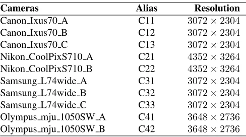
In this work, the noise residuals extracted by the methods of Lukas [1] and Kang [7] are used as original features. In order to evaluate the feasibility of the proposed method, these original features are given as inputs to the PCA-based feature extraction method [14] and the proposed method for the performance comparison. Hereafter, Lukas/Kang+PCA and Lukas/Kang+RSM indicate that the noise residuals are firstly extracted by Lukas/Kang method and the PCA-based feature extraction or the proposed RSM is performed afterwards. Our experiments are conducted on the Dresden Image database [17]. A total of 1200 images from 10 cameras are involved in the experiments, where each responsible for 120. These 10 camera devices belong to 4 camera models, each camera model has 2∼3 different devices. The cameras are listed in Table 1. All these images are natural images containing a wide variety of natural indoor and outdoor scenes. For each camera, 20 images are used for training and the remaining 100 are used as query images for testing. Thus, there are100×10
[image:4.612.315.559.586.722.2]intraclass and900×10interclass correlation values in total. We extract all the noise residuals from the luminance channel, as the luminance channel contains information of all the three channels. Our experiments are performed on an image block of 256×256 pixels cropped from the centre of a full size image.
Table 1: Cameras used in the experiments
Cameras Alias Resolution
Canon Ixus70 A C11 3072×2304
Canon Ixus70 B C12 3072×2304
Canon Ixus70 C C13 3072×2304
Nikon CoolPixS710 A C21 4352×3264
Nikon CoolPixS710 B C22 4352×3264
Samsung L74wide A C31 3072×2304
Samsung L74wide B C32 3072×2304
Samsung L74wide C C33 3072×2304
Olympus mju 1050SW A C41 3648×2736
L
0 100 200 300 400 500 600 700 800 900 1000 1100 1200 0
0.1 0.2 0.3 0.4 0.5 0.6 0.7 0.8 0.9
1 Canon Ixus70, M/d=0.5, 256x256 pixels, t=0.08
True positive rate False positive rate
Fig. 2: Performance with respect to the number of random subspaces
L.
M/d
0.1 0.2 0.3 0.4 0.5 0.6 0.7 0.8 0.9 1 0
0.1 0.2 0.3 0.4 0.5 0.6 0.7 0.8 0.9
1 Canon Ixus70, L=600, 256x256 pixels, t=0.08
True positive rate False positive rate
Fig. 3: Performance with respect to the dimension of the random subspaceM.
Flase positive rate
0 0.1 0.2 0.3 0.4 0.5 0.6 0.7 0.8 0.9 1
Ture positive rate
0.5 0.55 0.6 0.65 0.7 0.75 0.8 0.85 0.9 0.95
1 Overall ROC curves, 256x256 pixels
Lukas Lukas+PCA Lukas+RSM
Fig. 4: ROC curves of different variants of Lukas’ method [1].
Flase positive rate
0 0.1 0.2 0.3 0.4 0.5 0.6 0.7 0.8 0.9 1
Ture positive rate
0.5 0.55 0.6 0.65 0.7 0.75 0.8 0.85 0.9 0.95
1 Overall ROC curves, 256x256 pixels
Kang Kang+PCA Kang+RSM
Fig. 5: ROC curves of different variants of Kang’s method [7].
3.2. Performance evaluation
There are only two parameters in the proposed method,
namely, the dimension of random subspace M and the
number of random subspacesL. Figs. 2 and 3 show how the
true positive (false positive) rate of the method Lukas+RSM
vary for different values of M and L, respectively. As
shown in Fig. 2, the performance of the proposed method improves by increasing number of random subspaces. Since the performance tends to be stable whenL > 600and there is a tradeoff between the performance and the computational complexity, we setL= 600in the following experiments.
Fig. 3 indicates the sensitivity of the proposed method to
the parameterM, whereM is the dimension of each random
subspace anddis the size of the entire feature spaceT. It is worth mentioning that the performance of the proposed method is as same as that of the PCA-based extraction method
[14] whenM/d = 1. Therefore, from Fig. 3 we can see
that as long as M < d, the proposed method can achieve a higher true positive rate than the PCA-based extraction method. In addition, from both Figs. 2 and 3 we can see that the performance of the proposed method is not sensitive
toLandM. In rest of this paper, we empirically setL= 600
andM/d= 0.5, because these values yield the best result.
We use the Receiver Operating Characteristic (ROC) curve to compare the performance of different methods, as shown in Figs. 4 and 5. To get convincing results, all the
100×10intraclass and900×10interclass samples from 10 cameras are used together to draw the overall ROC curve [7]. However, the overall ROC curve for the proposed method is obtained in a slightly different manner. For a given detection threshold, we count the number of true positive decisions and the number of false positive decisions for each camera in each subspace, respectively and then sum them up to obtain the total number of true positive decisions and false positive decisions. Finally, the total True Positive Rate and total False Positive Rate are calculated to draw the overall ROC curve.
In Figs. 4 and 5, the black, blue, and red lines indicate
[image:5.612.329.534.76.230.2] [image:5.612.78.285.76.226.2] [image:5.612.324.534.272.427.2] [image:5.612.69.280.272.427.2]4. CONCLUSION
In the previous work [14], a feature extraction algorithm based on PCA denoising was proposed to extract a feature set with much lower dimensionality from the original noise resid-ual. However, the performance of this algorithm degrades when scene details are contained in the training set, as the obtained eigenvectors are affected by the scene details. As a result, some leading eigenvectors are more likely to represent the scene details rather than the real SPN signal. Moreover, since scene details may differ for different training samples, it is hard to locate and remove these corrupted eigenvectors from the feature space. To address these problems in this paper, an ensemble solution based on RSM and MV has been presented to randomly select subspaces from the PCA feature space to suppress the effect of scene details. The experimental results suggest that the proposed method has the capability to suppress the interference of scene details and achieves a superior ROC curve performance than both the original SPN extraction method and the PCA-based feature extraction method.
5. REFERENCES
[1] J. Lukas, J. Fridrich, and M. Goljan, “Digital camera identification from sensor pattern noise,” IEEE Trans. Inf. Forensics Security, vol. 1, no. 2, pp. 205–214, 2006.
[2] K. Dabov, A. Foi, V. Katkovnik, and K. Egiazarian, “Image denoising by sparse 3d transform-domain col-laborative filtering,” IEEE Trans. Image Process., vol. 16, no. 8, pp. 2080–2095, 2007.
[3] M. Chen, J. Fridrich, M. Goljan, and J. Lukas, “Deter-mining image origin and integrity using sensor noise,”
IEEE Trans. Inf. Forensics Security, vol. 3, no. 1, pp. 74–90, 2008.
[4] C.-T. Li, “Source camera identification using enhanced
sensor pattern noise,” IEEE Trans. Inf. Forensics
Security, vol. 5, no. 2, pp. 280–287, 2010.
[5] C.-T. Li and R. Satta, “Empirical investigation into the correlation between vignetting effect and the quality of sensor pattern noise,” IET Computer Vision, vol. 6, no. 6, pp. 560–566, 2012.
[6] C.-T. Li and Y. Li, “Color-decoupled photo response
non-uniformity for digital image forensics,” IEEE
Trans. Circuits Syst. Video Technol., vol. 22, no. 2, pp. 260–271, 2012.
[7] X. Kang, J. Chen, K. Lin, and A. Peng, “A context-adaptive spn predictor for trustworthy source camera
identification,” EURASIP Journal Image and Video
Processing, vol. 2014, no. 1, pp. 1–11, 2014.
[8] R. Li, C.-T. Li, and Y. Guan, “A reference estimator based on composite sensor pattern noise for source de-vice identification,” inProc. SPIE, Electronic Imaging, Media Watermarking, Security, and Forensics 2014, San Francisco, CA, USA, Feb. 2-6, 2014, vol. 9028.
[9] M. Goljan, “Digital camera identification from images - estimating false acceptance probability,” in Proc. Int. Workshop Digital-forensics and Watermarking, pp. 454–468. 2009.
[10] X. Kang, Y. Li, Z. Qu, and J. Huang, “Enhancing
source camera identification performance with a camera reference phase sensor pattern noise,” IEEE Trans. Inf. Forensics Security, vol. 7, no. 2, pp. 393–402, 2012.
[11] M. Goljan, J. Fridrich, and T. Filler, “Managing a
large database of camera fingerprints,” inProc. SPIE, Electronic Imaging, Media Forensics and Security XII, San Jose, CA, USA, Jan. 17C21, 2010, vol. 7541, pp. 08 01–12.
[12] Y. Hu, C.-T. Li, and Z. Lai, “Fast source camera
identification using matching signs between query and reference fingerprints,” Multimedia Tools and Applica-tions, pp. 1–24, 2014.
[13] S. Bayram, H. Sencar, and N. Memon, “Efficient sensor fingerprint matching through fingerprint binarization,”
IEEE Trans. Inf. Forensics Security, vol. 7, no. 4, pp. 1404–1413, 2012.
[14] R. Li, C.-T. Li, and Y. Guan, “A compact representation of sensor fingerprint for camera identification and fin-gerprint matching,” inProc. IEEE Int. Conf. Acoustics, Speech, and Signal Processing, Brisbane, Australia, Apr. 19-24, 2015, pp. 1777–1781.
[15] D. Zhang, R. Lukac, X. Wu, and D. Zhang, “PCA-based spatially adaptive denoising of CFA images for single-sensor digital cameras,” IEEE Trans. Image Process., vol. 18, no. 4, pp. 797–812, 2009.
[16] Y. Guan, C.-T. Li, and F. Roli, “On reducing the effect of covariate factors in gait recognition: A classifier
ensemble method,” IEEE Trans. Pattern Anal. Mach.
Intell., vol. 37, no. 7, pp. 1521–1528, 2015.
[17] T. Gloe and R. B¨ohme, “The Dresden image database
for benchmarking digital image forensics,” Journal

![Fig. 4: ROC curves of different variants of Lukas’ method [1].](https://thumb-us.123doks.com/thumbv2/123dok_us/9516668.457119/5.612.324.534.272.427/fig-roc-curves-different-variants-lukas-method.webp)
