Principal component and factor analysis to study variations in the aging lumbar spine

http://wrap.warwick.ac.uk

Original citation:

Khan, Atif A., Iliescu, Daciana, Sneath, R. J. S., Hutchinson, Charles and Shah, A. A..

(2015) Principal component and factor analysis to study variations in the aging lumbar

spine. IEEE Journal of Biomedical and Health Informatics, Volume 19 (Number 2). pp.

745-751. ISSN 2168-2194

Permanent WRAP url:

http://wrap.warwick.ac.uk/60393

Copyright and reuse:

The Warwick Research Archive Portal (WRAP) makes this work by researchers of the

University of Warwick available open access under the following conditions. Copyright ©

and all moral rights to the version of the paper presented here belong to the individual

author(s) and/or other copyright owners. To the extent reasonable and practicable the

material made available in WRAP has been checked for eligibility before being made

available.

Copies of full items can be used for personal research or study, educational, or not-for

profit purposes without prior permission or charge. Provided that the authors, title and

full bibliographic details are credited, a hyperlink and/or URL is given for the original

metadata page and the content is not changed in any way.

Publisher’s statement:

“© 2014 IEEE. Personal use of this material is permitted. Permission from IEEE must be

obtained for all other uses, in any current or future media, including reprinting

/republishing this material for advertising or promotional purposes, creating new

collective works, for resale or redistribution to servers or lists, or reuse of any

copyrighted component of this work in other works.”

A note on versions:

The version presented here may differ from the published version or, version of record, if

you wish to cite this item you are advised to consult the publisher’s version. Please see

the ‘permanent WRAP url’ above for details on accessing the published version and note

that access may require a subscription.



Abstract— Human spine is a multifunctional structure of

human body consisting of bones, joints, ligaments and muscles which all undergo a process of change with the age. A sudden change in these features either naturally or thorough injury can lead to some serious medical conditions which puts huge burden on health services and economy. While aging is inevitable, the effect of aging on different areas of spine is of clinical significance. This paper reports the growth and degenerative pattern of human spine using principal component analysis. Some noticeable lumbar spine features such as vertebral heights, disc heights, disc signal intensities, para-spinal muscles, subcutaneous fats, psoas muscles and cerebrospinal fluid were used to study the variations seen on lumbar spine with the natural aging. These features were extracted from lumbar spine magnetic resonance images of 61 subjects with age ranging from 2 to 93 years. Principal component analysis is used to transform complex and multivariate feature space to a smaller meaningful representation. PCA transformation provided 2D visualization and knowledge of variations among spinal features. Further useful information about correlation among the spinal features is acquired through factor analysis. The knowledge of age related changes in spinal features are important in understanding different spine related problems.

Index Terms— Age related changes, data mining, dimension

reduction, factor analysis, lumbar spine, magnetic resonance imaging (MRI), principal component analysis.

I. INTRODUCTION

ATA mining has great potential for exploring the hidden patterns in medical data sets. These patterns can be utilized for clinical diagnosis and understanding disease prevalence. However, most of the available raw medical data sets are huge, widely distributed, complex and heterogeneous in nature. This makes medical data mining more rigorous and complex to handle. Whether it is genomics, study of human brain dynamics, analysis of biological relationships, image

Manuscript revised on: 31st _{Dec 2013. This work was partially supported}

by the “Warwick Impact Fund”, University of Warwick, Coventry UK. A.A. Khan is with Intelligent Systems Engineering Laboratory, School of Engineering, University of Warwick, Coventry, CV4 7AL, United Kingdom ([email protected]).

D.D. Iliescu is with School of Engineering, University of Warwick, Coventry, CV4 7AL, United Kingdom ([email protected])

R.J. Sneath is with University Hospital Coventry and Warwickshire, Clifford Bridge Road Coventry, CV2 2DX, UK ([email protected]). C.E. Hutchinson is with Clinical Sciences Research Laboratories, Warwick Medical School, University Hospital Coventry and Warwickshire, Clifford Bridge Road, Coventry, CV2 2DX, UK ([email protected]).

A.A. Shah is with School of Engineering, University of Warwick, Coventry, CV4 7AL, United Kingdom ([email protected]).

informatics, study of infectious disease or disease diagnosis, data mining finds its application in almost all areas of biomedicine [1].

Aging in humans is a multidimensional process of physical, psychological and social change in a person over time. Some dimensions of aging grow and expand over time, while others decline. The aging of the population in developed countries appears to be a non-reversible phenomenon. Decreased birth rates and increased life expectancy have risen the median age [2]. This increasing median age has significant social and economic implications in general, with tremendous load on healthcare services. With the aging population increased numbers of musculoskeletal problems are seen. Back and neck pain are among the most frequently encountered complaints of older people [3]. Back pain is usually associated with spine problems. The nature of the spine makes those problems highly complex to investigate and treat. The unrelenting changes associated with aging gradually affect almost all areas of the spine.

In the modern world, the use of magnetic resonance imaging (MRI) for diagnosing back pain and other spine problems has become a standard practice. Clinical specialists have an extensive amount of information these days, ranging from details of clinical symptoms to various types of biochemical data and outputs of imaging devices. With the help of MRI, the underlying anatomical reason for back pain and spinal pathology can be sought. In the absence of pathology such as fracture, tumor or infection, back pain is commonly thought to come from the intervertebral discs, the facet joints, muscles, tendinous or ligamentous insertions of the lumbar spine. However, when there is no pathological indication from MRI, patients remain frustrated about the cause of their back pain. Therefore one of the reasons to conduct this study is to explore beyond the apparent lack of anatomical indications and reveal ‘hidden’ information with the help of principal component and factor analyses. Back pain sometime originates due to age related degenerative changes in the spine. Spine specialists do not have any reference values to compare with patients’ age and reassure them that the result of their MRI is not indicative of any disease and the aging effect on their spines is within natural limits. In this paper, information extracted from lumbar spine MRIs is used to visualize and correlate the changes seen in human lumbar spine features with aging. This study will be helpful in understanding changing characteristics of lumbar spine with the natural aging. By finding the significance and correlation among spinal features, clinicians will be able to

Principal Component and Factor Analysis to

Study Variations in the Aging Lumbar Spine

A.A. Khan*, D.D. Iliescu, R.J. Sneath, C.E. Hutchinson and A.A. Shah

understand the spinal disease prevalence in a better way. The results from this study will also be helpful in finding the correlation between changing anatomy of spine and back pain.

In this paper the appearance and variation of several key spine structures are reported in detail. In general, when the appearance of these structures seems to vary with age, they are often described as degenerative or age related changes (ARCs). To date, there are no standard reference values available which can be compared to conclude whether the changes in spinal features are induced by natural aging or by some disease. Some studies have tried to explore the effect of aging on specific areas of the spine but the findings vary among the studies. For example some studies suggest vertebral height increase with the age [4] while other reports decrease in vertebral height with the age [5]. Interestingly, another study suggests that vertebral body size increases with age in males but remains the same for females [6]. Some studies have confirmed a correlation of spinal variations with age [7]-[9] whereas some others have failed to do so [10], [11]. In some studies, when looking at specific aspects of the scan, there seems to be an extremely strong correlation with age [12], [13]. A handful of studies are carried out to understand the aging effect on lumbar spine. Most of them, explore the behavior of a single feature at a time. But due to the complex nature of the spine, many of the spinal features are interconnected and often move together. So looking at one feature may not always give an accurate picture.

Some studies tried to correlate age related changes to clinical symptoms but with few succeeding [14]. There is a general agreement that changes induced by aging lead to alterations in the thickness of the disc and muscles [15], but there are differences in the accounts of the effect of aging on the thickness of the lumbar discs. One study stressed that reduction of the intervertebral disc height with age is inevitable [16]. In contrast, an increase in disc height with age has been reported by other study [17]. One study suggests that disc degeneration is highly correlated with age and educational level [18]. Similarly, many others have tried to link spinal aging with environment and genetics. According to another study, the only degenerative feature associated with self-reported lower back pain was spinal stenosis [19]. Some studies suggest that there is a significant difference in pattern of vertebral growth in male and female [20], [21]. Therefore, the variation in the incidence of ARC’s varies widely between the studies. The method of assessing ARC’s also varies widely from ordinal observer data to continuous, computer generated data. The number and type of ARC’s varies but are often presented to mean the same in regards the amount of degeneration seen on the lumbar spine MRI. The variations among the studies are due to the way of looking at the data. Most of the studies have tried to correlate one feature at a time. Very few have tried to correlate two or more spinal features with aging process. The spine is a complex structure having several bones, ligaments, joints and muscles which often affect one another and move together. So it is important to study the group of spinal features simultaneously. This research is based on the evaluation of 24 spinal features

simultaneously against the natural aging. This work not only portrays the behavior of an individual feature of the spine but also explores the correlation among the features.

II. MATERIALS AND METHODS

A. Overview

In this paper information from lumbar spine MRIs is used to visualize the variations in human lumbar spine among different age groups. A human spine consists of bones, joints, ligaments and muscles. There are a total of 33 vertebrae in the human spine: 7 in the neck (cervical region), 12 in the middle back (thoracic region), 5 in the lower back (lumbar region), 5 that are fused to form the sacrum and the 4 coccygeal bones that form the tailbone. Mechanical back pain usually comes from the lumbar spine, so this paper focuses on lumbar spine area for the pilot study. The lumbar spine has five vertebrae, namely L1, L2, L3, L4, L5 separated by intervertebral discs. Fig. 1 shows sagittal (left) and an axial (right) view of the lumbar spine MRI.

Fig. 1. Sagittal (left) and an axial (right) view of the lumbar spine MRI

B. Data Set

The data set used in this pilot study was taken from University Hospital Coventry and Warwickshire NHS Trust, Coventry, United Kingdom in the form of patient MRIs. All the necessary ethical approvals were obtained from the concerned bodies against the use of data for research purposes. Images were obtained from GE Scanners (GE healthcare Milwaukee) at 1.5T using standard imaging protocol. All the subjects were scanned in supine position. Images were visualized and scored using the PACS web browser (GE). The format of data was digital imaging and communications in medicine (DICOM). An attempt was made to keep only MRI scans which do not exhibit any clearly visible lumbar spine pathology. However, no assessment was made into the patients clinical symptoms.

Fig. 2. Distribution of data samples

C. Feature Extraction, Measurement and Scoring of Data

There are several features that can be studied from a lumbar spine MRI scan. After a thorough literature study, a list of significant lumbar spine features was prepared by the orthopedic spinal surgeon and radiologist for the pilot study. The scoring criteria were set to look initially at vertebral heights (L1, L2, L3, L4, L5), disc heights (T12-L1, L1-L2, L2-L3, L3-L4, L4-L5, L5-S1), disc signal intensities (T12-L1, L1-L2, L2-L3, L3-L4, L4-L5 and L5-S1), para-spinal muscle signal intensity at L3 (both left and right), subcutaneous fat left and right, psoas muscle (both left and right) and cerebrospinal fluid (CSF). These 24 spinal features were used in principal component and factor analysis. Although there are tools and procedures available for automated segmentation and feature extraction [22], [23], in this pilot study, features were measured manually by an orthopedic spinal surgeon using digital measuring tools. The measurements were repeated twice to get a good approximate and were recorded against lumbar spine MRIs of the 61 subjects. Vertebral and disc heights were measured from the center of vertebras and discs and were reported in millimeters.

III. PRINCIPAL COMPONENT ANALYSIS

One of the inherent difficulties in multivariate analysis is the problem of visualizing data that has many variables. In such datasets, groups of variables often move together and usually measure the same driving principle governing the behavior of the system [24]. In such scenarios, one can take advantage of this redundancy of information. This problem can be simplified by replacing a group of variables with a single new variable [25]. Humans often have difficulty comprehending data that has many dimensions. Thus, reducing data to a small number of dimensions is useful for visualization purposes. With a large number of variables in a dataset, the dispersion matrix may be too large to study and interpret. There would be too many pairwise correlations between the variables to consider. Graphical display of data may not be of particular help in case the data set is very large. For example, with 12 variables, there will be 220 three-dimensional plots to be studied. To interpret the data in a meaningful form, it is therefore necessary to reduce the number of variables to a few, interpretable linear combinations of the data, where each linear combination will correspond to

a principal component [26], [27]. Principal components analysis is a quantitatively rigorous method for achieving this simplification. The full set of principal components is as large as the original set of variables. But it is commonplace for the sum of the variances of the first few principal components to exceed 80% or so of the total variance of the original data [28], [29]. By examining plots of these few new variables, researchers often develop a deeper understanding of the driving forces that generated the original data.

PCA is mathematically defined as an orthogonal linear transformation that transforms the data to a new coordinate system such that the greatest variance by any projection of the data comes to lie on the first coordinate (called the first principal component), the second greatest variance on the second coordinate, and so on [30]. In PCA, one wishes to extract from a set of p variables a reduced set of m

components that accounts for most of the variance in the p

variables. PCA is completely reversible and the original data can be recovered from the principal components, making it a versatile tool, useful for data reduction, noise rejection, visualization and data compression. In this paper, the dimension of the original data is reduced by a factor of eight, without losing much information. Multivariate data set is visualized by making 2D plots and relationships among the spinal features were understood by studying these plots. This work provides an easy to understand visual representation of spinal feature variations with age. For the principal component analysis, all 24 scored features of lumbar spine were considered. These features were measured against 61 selected subjects.

A. Statistical Analysis and Data Standardization

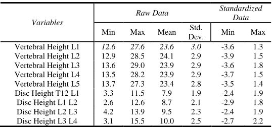
Usually principal components are computed from raw data when all the variables in the dataset have the same units. Standardization of data is often preferable when the variables are in different units or when variance of the different columns is substantial as in this case. If the standard deviations of variables are different from one another, then one variable might dominate in the analysis [31]. Equation 1 gives the standardization formula used in PCA analysis, where is the original observed data value, is the mean and is the standard deviation. The statistics of raw and standardized data is shown in Table 1.

TABLE 1

STATISTICS OF RAW AND STANDARDIZED DATA

Variables

Raw Data Standardized

Data

Min Max Mean Std.

Disc Height L4 L5 2.2 16.9 9.5 3.0 -2.4 2.4 Disc Height L5 S1 1.6 14.4 9.1 2.7 -2.8 2.0 Disc Signal T12 L1 28.0 374.5 119.2 78.4 -1.2 3.3 Disc Signal L1 L2 20.9 373.4 126.4 79.5 -1.3 3.1 Disc Signal L2 L3 26.7 436.8 118.1 80.4 -1.1 4.0 Disc Signal L3 L4 28.4 460.0 118.9 85.0 -1.1 4.0 Disc Signal L4 L5 28.6 473.0 115.7 84.9 -1.0 4.2 Disc Signal L5 S1 21.9 374.2 110.0 85.5 -1.0 3.1 Paraspinal Muscle Right 14.1 405.5 135.4 85.6 -1.4 3.2 Paraspinal Muscle Left 16.4 303.3 128.4 71.9 -1.6 2.4 Psoas Muscle Right 25.3 150.2 66.6 25.6 -1.6 3.3 Psoas Muscle Left 21.5 169.4 64.7 28.5 -1.5 3.7 Subcutaneous Fat Right 167.4 836.3 510.7 174.3 -2.0 1.9 Subcutaneous Fat Left 159.7 961.7 547.3 167.2 -2.3 2.5 CSF at L3 186.7 1316 561.1 215.0 -1.7 3.5

B. Data Visualization

The principal components were computed using the variance technique [32]. Using Matlab Statistical Toolbox, 24 components were computed from 24 original features. Fig. 3 shows the first five components. It can be seen that most of the variance (88.5%) in data is shown by the first three components. The first component accounts for 36.08% variance, the second component accounts for 31.64% and the third component accounts for 20.78% of the variance in whole data. As 88.5% of the variance is explained by the first three components, the remaining components can be excluded or discarded. With PCA, 24 features were now replaced by 3 principal components. The size of the original data set was reduced from 61x24 to 61x3. By compressing the original data 8 times, only 11.5% information is lost. Using these three principal components, original data can be easily visualized using a single 3D plot or making three 2D plots (1st vs. 2nd component, 1st vs. 3rd component, and 2nd vs. 3rd component).

Fig. 3. Variance shown by first 5 components of the data

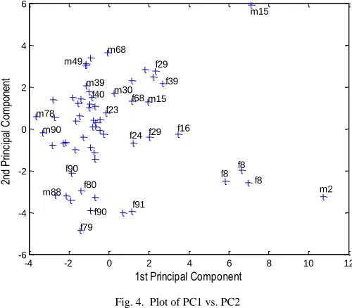
A plot of first versus second principal component that account for about 68% of the variance in the data is shown in Fig 4. It shows the distribution of the 61 subjects ranked on the basis of their spinal scores. Each “+” sign corresponds to a specific subject. It can be seen that most of the subjects were dragged on the left side of the first principal component whereas second principal component has almost an equal distribution of the subjects.

Fig. 4. Plot of PC1 vs. PC2

Each subject was labelled with the corresponding age and gender to explore the patterns in the data. Fig. 4 shows the plot of first two principal components labelled with their age and gender. It can be seen that as we move along the first principal component, age tends to change. Subjects with age 2, 8, 15, 16 etc. are located in the right or the positive half whereas subjects with age 68,78,88,90,91 etc. are located in the left most or negative half of the first principal component. So it can be said that the first principal component is the descriptor for age. Also, it can be seen that the most of the subjects in the positive (upper) half of the second principal component are male whereas most of the subjects in negative (lower) half of the second principal are female. Though there are few exemptions but it can be fairly said that second principal component is descriptor for the gender. Fig. 5 shows the plot of first principal component versus age. It can be seen that the age increases as we move from positive to the negative half of the first principal component.

Fig. 5. 1st _{principal component vs. age}

1 2 3 4 5

0 10 20 30 40 50 60 70 80 90 100 Principal Component Va ria nc e Ex pl ai ne d (% ) 0% 10% 20% 30% 40% 50% 60% 70% 80% 90% 100% C um ul at iv e Va ria nc e

-4 -2 0 2 4 6 8 10 12

-6 -4 -2 0 2 4 6

1st Principal Component

2n d Pr in ci pa l C om po ne nt f8 f8 f8 m2 f16 f29 f24 f79 f90 f80 f90 f91 m88 m78 m15 f39 m30 f68 f23 m68 m90 m39 f40 f29 m49 m15

-4 -2 0 2 4 6 8 10 12

0 10 20 30 40 50 60 70 80 90 100

1st Principal Component

A g e 78 69 69 68 ₆₈ 58 58

39 40₃₉

30 30 29

The plot of PC1 vs. PC3 is shown in Fig. 6. Again principal component 1 here is the descriptor for age. Principal component three has greater concentration of female subjects in the middle of axis or close to zero whereas male subjects tend to lie away from zero, either between: 1 to 4 or -1 to -4.

Fig. 6. Plot of PC1 vs. PC3

The plot of second and third principal components is shown in Fig. 7. Principal component two shows a gender bias as majority of male subjects lie on the positive half and majority of female subjects lie on the negative half of component two. Component three has a mixed distribution of subjects which does not provide much information.

Fig. 7. Plot of PC2 vs. PC3

C. Correlated Features

Reducing the dimensions of the data and plotting the principal components gives an understandable visual representation of the data. This 2D representation uncovers some patterns in the data but more knowledge can be extracted by exploring the driving force with allocates or ranks the samples in 2D plane. Plotting first vs. second principal component and exploring the driving force for the allocation of sample provides the significance of the variables. Plot of

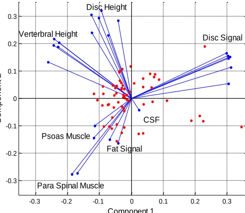
samples and variables for principal component one and two (accounting for 68% variance) is shown in Fig. 8. Each blue line in this figure represents the corresponding variables as labelled. The magnitude of line gives the significance of that variable. The most significant here is disc signal intensities located in the first quadrant. The other significant variables are vertebral heights and disc heights located in the second quadrant. In third quadrant, para spinal muscle signal intensity shows high significance whereas fat signals and psoas signal shows somewhat lesser significance. The least significant is CSF, found in fourth quadrant.

Fig. 8. Plot of samples and correlated variables

Fig. 8 not only gives the significance of the input variables but also provides the correlation among the input variables. Looking into first quadrant, it can be seen that disc signal intensities (T12-L1, L1-L2, L2-L3 and L3-L4) are almost overlapping each other showing that these variables are correlated and show similar pattern. Disc signal intensities L4-L5 and L4-L5-S1 show a little different behaviour than the rest. Similarly, by looking at the vertebral heights in second quadrant, L1, L2, L3, and L4 are very close to one another whereas L5 is bit away from them. This shows that the aging pattern of vertebra L5 is slightly different from the rest of lumbar vertebrae. It can also be seen from Fig. 8 that the behaviour of disc height L1-L2 resembles more to L3-L4 than the L2-L3. Also, disc height L4-L5 is located slightly away from the rest. Disc height L5-S1 is the least significant lumbar disc height. In third quadrant, para spinal muscle signal intensities left and right are close to one another. It can also be noticed that pattern of psoas left and fat signal left is slightly different from psoas right and fat signal right.

Here we have seven set of input variables as vertebral heights, disc heights, disc signal intensities, psoas signal, fat signal, para-spinal muscle signal intensities and CSF. These features are said to be somehow interconnected and affect each other. An interesting thing about PCA representation (given in Fig. 8) is that we can draw conclusion about the existing correlation among these set of variables. The variables located in the same quadrant are said to be correlated

-4 -2 0 2 4 6 8 10 12

-4 -3 -2 -1 0 1 2 3 4

1st Principal Component

3r d Pr in ci pa l C om po ne nt m15 f8 f8 f8 m2 f16 m78 f68 m91 m90 m39 m88 m16 m30 m58 m30 m49 f29 m15 f16 f91 f89 f39 f29 f59 m58 f53 m17 f23 f68 f49 f59 m68 f58 f90 f69

-6 -4 -2 0 2 4 6

-4 -3 -2 -1 0 1 2 3 4

2nd Principal Component

3r d Pr inc ipa l C om po ne nt f90 m90 f90 f89 m88 f80 f80 m80 f79 m80 f79 m78 f69 f69 f69 f69 m68 m68

f59 _f59m58

m58 m49 f50 f49 m49 m39 f40 f40 m40 m39 m30 f29 m30 m17 m16 m15 m15 f8 f8 f8 f92 m91 m91 f91 f90 m93 f24 f68

-0.3 -0.2 -0.1 0 0.1 0.2 0.3

-0.3 -0.2 -0.1 0 0.1 0.2 0.3 Disc Signal Disc Height Verterbral Height

and move together. The variables which are located in adjacent quadrant (or are at right angle) have no effect each other. And the variables in the opposite quadrant are negatively correlated to each other. In other words, if one increases the other one decreases. From Fig. 8, vertebral heights and disc heights lie in the same quadrant and therefore are correlated. Similarly, psoas signal, fat signal and para spinal muscle signal intensity are also correlated.

D. Non Correlated Features

The magnitude of blue lines gives the significance of the respective variable with aging. It can be seen from Fig. 8 that CSF is the least significant variable. Disc signal intensities, psoas signal, fat signal, and para-spinal muscle signals are located adjacent to CSF meaning that they have no correlation with CSF. However, CSF has negative correlation with vertebral heights and disc heights. Similarly, disc signal intensities have a negative correlation with psoas signal, fat signal, and para-spinal muscle signal. Vertebral and disc heights have no correlation with disc signal, psoas signal, fat signal, and para-spinal muscle. It was concluded that CSF shows the least variations with natural aging.

IV. FACTOR ANALYSIS

Factor analysis is a statistical method used to describe variability among observed, correlated variables in terms of a potentially lower number of unobserved variables called factors [33]. Factor analysis and principal component analysis are related to each other but are not identical [34]. Principal components analysis is commonly used to find optimal ways of combining variables into a small number of subsets, whereas factor analysis is commonly used to identify the structure underlying such variables and to estimate scores to measure latent factors themselves [35]. A generic correlation among the variables is presented in the previous section. In this section, factor analysis is used to get the numerical values of the significance and correlation seen among the features.

Factor analysis was also conducted in Matlab Statistical toolbox. Three principal factors were extracted from data set. Looking at the loadings of factor one, it was found that disc signal intensities were the most significant feature which varies with the age. A general rule of thumb is that any variable having loading value greater than or equal to 0.7 is said to be significant. However, this level is said to be very high and most of the researchers use 0.4 as an appropriate level for real life data analysis. In this analysis, any variable scoring greater than 0.7 are supposed to be highly significant. Variables with loadings between 0 - 0.2 are treated as non-significant. Variables with loading values between 0.2 - 0.7 are somewhat significant. Loadings for factor one in the order of their significance is given in table 2, with disc signal L2-L3 being the most significant of all. Each factor has loadings for all 24 variables but here only the non-zero values are shown.

TABLE 2

NON-ZERO LOADINGS OF FIRST FACTOR

Variables Factor Loadings Disc Signal L2 L3 0.99155 Disc Signal L3 L4 0.98236 Disc Signal L1 L2 0.97114 Disc Signal T12 L1 0.92710

Disc Signal L4 L5 0.88377 Disc Signal L5 S1 0.77728 Para Spinal Muscle Left -0.58326 Para Spinal Muscle Right -0.52695 Psoas Muscle Right -0.24495 Psoas Muscle Left -0.22365 Subcutaneous Fat Signal Right -0.18871 Subcutaneous Fat Signal Left -0.18790 Cerebrospinal Fluid 0.15359

This shows that para spinal muscle signal intensity left-right, psoas left-tight, and fat left-left-right, are negatively correlated with disc signal intensities. Since the factor loadings for fat signal and CSF is very low, so it can be said that they are non-significant variables and they do not vary a lot with the age. Psoas and para-spinal muscles are somewhat significant. The most significant variables are of disc signal intensities. Similarly, looking at the loading of factor two, vertebral heights is the only set of variables which are significant. All other variables have very small loading values which can be neglected. The loadings for factor two in the order of their significance are given in table 3 below.

TABLE 3

TOP FIVE LOADINGS OF SECOND FACTOR

Variables Factor Loadings Vertebral Height L3 0.99457 Vertebral Height L2 0.94146 Vertebral Height L4 0.93064 Vertebral Height L1 0.88570 Vertebral Height L5 0.85394

By inspecting the loadings of factor three, disc heights are the most significant variables. They are listed in table 4 below, on the basis of their significance.

TABLE 4

TOP SIX LOADINGS OF THIRD FACTOR

Variables Factor Loadings Disc height L2 L3 0.89957 Disc height L3 L4 0.88404 Disc height L1 L2 0.81926 Disc height L4 L5 0.75404 Disc height L5 S1 0.66527 Disc height T12 L1 0.63065

V. CONCLUSION AND FUTURE WORK

analysis was that the relationships between all of the variables in the model were examined simultaneously and also in pair-wise combinations.

Some interesting patterns were observed from multivariate analysis. Disc signal intensities were found to have a very strong correlation with natural aging. Disc signal L2-L3 is the one most affected by the aging. Disc heights and vertebral heights also show a strong correlation with natural aging. Vertebral height L3 and disc height L2-L3 were most prominent in their respective groups. Para-spinal muscles show a moderate correlation with age; with left muscle scoring slightly higher than right one. Psoas muscle shows a very little correlation whereas subcutaneous fat signal and cerebrospinal fluid (CSF) were almost non-correlated with age. Disc heights and vertebral heights were found correlated to each other. Similarly, psoas, para spinal muscle, and fat signals were also found correlated and have a negative correlation with disc signal intensities.

This research was based on the scores of 24 spinal features. However, in addition to these 24 features, some other notable features such as; Schmorl’s nodes, Modic changes, vertebral alignment, osteophytes, ligamentum flavum, and facet joints will also be considered for future analysis.

REFERENCES

[1] H. Chen, S. S. Fuller, C. Friedman, W. Hersh, "Knowledge management, data mining, and text mining in medical informatics," Medical Informatics, pp. 3-33. Springer US, 2005.

[2] World Population Program, Population Research at International Institute for Applied Systems Analysis (IIASA), Luxemburg, Austria. http://www.iiasa.ac.at/web/home/research/Population.en.html

[3] J. Fricker, "Pain in Europe—a 2003 report." Mundipharma International Ltd, Cambridge. Retrieved from http://www. britishpainsociety.org [4] T. Videman, M.C. Battié, L.E. Gibbons, K. Gill, “Aging Changes in

Lumbar Discs and Vertebrae and Their Interaction A 15-year Follow-up Study”, The Spine Journal, 2005.

[5] D. Diacinti, M. Acca, E. D'Erasmo, E. Tomei, G.F. Mazzuoli,, “Aging changes in vertebral morphometry,” Calcified tissue international, vol. 57, no. 6, pp. 426-429, 1995.

[6] L. Mosekilde, L. Mosekilde, “Sex differences in age-related changes in vertebral body size, density and biomechanical competence in normal individuals,” Bone, vol. 11, no. 2, 67-73, 1990.

[7] M.C. Battié, T. Videman. "Lumbar disc degeneration: epidemiology and genetics," Bone Joint Surg., vol. 88, no. 2, pp. 3-9, Apr. 2006.

[8] T. Videman, M.C. Battié, K. Gill, H. Manninen, L.E. Gibbons, L.D. Fisher, "Magnetic resonance imaging findings and their relationships in the thoracic and lumbar spine: insights into the etiopathogenesis of spinal degeneration," Spine, vol. 20, no. 8, pp. 928-935, Apr. 1995. [9] N. Boos, S. Weissbach, H. Rohrbach, C. Weiler, K.F. Spratt, A.G.

Nerlich, "Classification of age-related changes in lumbar intervertebral discs: 2002 Volvo Award in basic science," Spine, vol. 27, no. 23, pp. 2631-2644, Dec. 2002.

[10] A. Sharma, M. Parsons, T. Pilgram, "Temporal interactions of degenerative changes in individual components of the lumbar intervertebral discs: A sequential magnetic resonance imaging study in patients less than 40 years of age," Spine, vol. 36, no. 21, pp. 1794-1800, Oct. 2001.

[11] J.A.A. Miller, C. Schmatz, A.B. Schultz, “Lumbar disc degeneration: correlation with age, sex, and spine level in 600 autopsy specimens,” in Spine, vol. 13, no. 2, pp. 173-178, 1998.

[12] T. Videman, L.E. Gibbons, M.C. Battié, "Age-and pathology-specific measures of disc degeneration," Spine, vol. 33, no. 25, pp. 2781-2788, Dec. 2008.

[13] R. Niemeläinen, T. Videman, S.S. Dhillon, M. C. Battié, "Quantitative measurement of intervertebral disc signal using MRI," Clin. Radiol., vol. 63, no. 3, pp. 252-255, Mar. 2008.

[14] K.M. Cheung, J. Karppinen, D. Chan, D.W. Ho, Y.Q. Song, P. Sham, K.D. Luk, "Prevalence and pattern of lumbar magnetic resonance imaging changes in a population study of one thousand forty-three individuals," Spine, vol.34, no. 9, pp. 934-940, Apr. 2009.

[15] R. Parkkola, M. Kormano, “Lumbar disc and back muscle degeneration on MRI: correlation to age and body mass,” Journal of Spinal Disorders & Techniques, vol. 5, no. 1, pp. 86-92, 1992.

[16] B.V. Roberts, "Disc pathology and disease states," The biology of the intervertebral disc, 2nd ed., pp. 73-119, 1998.

[17] Z. Shao, G. Rompe, M. Schiltenwolf, "Radiographic changes in the lumbar intervertebral discs and lumbar vertebrae with age," Spine, vol. 27, no. 3, pp. 263-268, Feb. 2002.

[18] B.E. Igbinedion, A. Akhigbe, “Correlations of radiographic findings in patients with low back pain,” Nigerian medical journal: journal of the Nigeria Medical Association, vol. 52, no. 1, pp. 28, 2011.

[19] L. Kalichman, D.H. Kim, L. Li, A. Guermazi, D.J. Hunter, “Computed tomography–evaluated features of spinal degeneration: prevalence, intercorrelation, and association with self-reported low back pain,” The spine journal, vol. 10, no. 3, pp. 200-208, 2010.

[20] P. Geusens, J. Dequeker, A. Verstraeten, J. Nijs "Age-, sex-, and menopause-related changes of vertebral and peripheral bone: population study using dual and single photon absorptiometry and radiogrammetry," Journal of nuclear medicine: official publication, Society of Nuclear Medicine, vol. 27, no. 10, pp. 1540-1549, 1986. [21] Y. Duan, C.H. Turner, B.T. Kim, E. Seeman, “Sexual Dimorphism in

Vertebral Fragility Is More the Result of Gender Differences in Age‐Related Bone Gain Than Bone Loss,” Journal of Bone and Mineral Research, vol. 16m no. 12, pp. 2267-2275, 2001.

[22] J. Carballido-Gamio, S.J. Belongie, S. Majumdar, "Normalized cuts in 3-D for spinal MRI segmentation," IEEE Trans. Med. Imag., vol. 23, no. 1, pp. 36-44, Jan 2004.

[23] Y. Zheng, M.S. Nixon, R. Allen, "Automated segmentation of lumbar vertebrae in digital videofluoroscopic images," IEEE Trans. Med. Imag., vol. 23, no. 1, pp. 45-52, Jan. 2004.

[24] J.E. Jackson, "A User’s guide to principal components,” John Willey Sons Inc, New York, 1991.

[25] W.J. Krzanowski, "Principles of multivariate analysis—a user’s perspective”, Revised ed., Oxford University Press, 2000.

[26] Online course material, STAT-505, “Applied Multivariate Statistical Analysis, Lesson 7: Principal Components Analysis (PCA)”, The Pennsylvania State University. USA.

[27] H. Abdi, L.J. Williams, "Principal component analysis," Wiley Interdisciplinary Reviews: Computational Statistics, no. 2, pp. 433–459, 2010.

[28] I.T. Jolliffe, “Principal Component Analysis”, Springer Series in Statistics, 2nd _{ed., Springer, NY, 2002, XXIX, ISBN 978-0-387-95442-4.}

[29] I. Jolliffe, “Principal component analysis”, John Wiley & Sons Ltd, 2005.

[30] B. Jones, “MATLAB: Statistics Toolbox User's Guide,” MathWorks, 1993.

[31] D.D. Suhr, "Principal component analysis vs. exploratory factor analysis," SUGI30 Proceedings, Philadelphia, USA, Apr. 10-13, pp. 203-230.

[32] J. Shlens, "A tutorial on principal component analysis," Systems Neurobiology Laboratory, University of California at San Diego, 2005. [33] G.V. Belle, L.D. Fisher, P.J. Heagerty, T. Lumley, “Principal

Component Analysis and Factor Analysis,” Biostatistics: A Methodology for the Health Sciences,” Second Edition, 2004, pp. 584-639.

[34] W.L. Martinez, A. Martinez, J. Solka, “Exploratory data analysis with MATLAB”, CRC Press, 2004.