Munich Personal RePEc Archive
Methods of choosing the most profitable
real assets among options that require
different amounts for various periods of
time
Kogan, Anton
Novosibirsk State University of Architecture and Civil Engineering
10 January 2013
Online at
https://mpra.ub.uni-muenchen.de/47928/
Methods of Choosing The Most Profitable Real Assets Among Options That Require Different Amounts For Various Periods of Time
ANTON KOGAN1 © 2013
ABSTRACT
The article deals with the indicators used when making investment decisions in situations when it is
necessary to invest different amounts of money in alternative real assets for different periods of time. The
author suggests two new indicators: “the indicator of the speed of specific increment in value” ( ) and
“conditional bank deposit” ( . The first indicator is used to choose the best investments that bring
some profit. The second indicator is used to choose the best investments that do not directly bring profit,
but are required for the operation of the company.
The existing methods used to choose the best variant for real investments have been
developed during several decades. To solve this task, such indicators as net present value ( ),
internal rate of return ( ), profitability index ( ), modified internal rate of return ( ),
payback period ( ), equivalent annual annuity ( ), equivalent annual cost ( ). All these
indicators have been thoroughly developed for three cases:
1) several alternative real assets are compared, in which the same amount is invested for
the same period of time;
2) several options are compared, in which the same amount is invested but for different
periods of time\terms;
3) several options are compared, in which different amounts are invested for the same
period of time.
1
Candidate of Economic Science, Associate professor of the Chair of Construction Economics and Investments in
Novosibirsk State University of Architecture and Civil Engineering. The author thanks Alexey Shirokikh for
In the meanwhile, there is a fourth case when it is necessary to compare alternatives
where both amounts and terms are different. All the above mentioned indicators do not apply in
such a situation. Let us specify that this work analyzes making of investment decisions in a
commercial company. That means that the investment project is described by the net cash flow
( ) that does not include macroeconomic effects.
To do further analysis, let’s divide real investments into two categories: money-gaining
and money-losing investments. Money-gaining investments bring in returns (for example, a
company buys some equipment to manufacture building products with their subsequent sale).
Money-losing investments do not participate in the formation of the profit directly, but they are
required in the business (for example, the company buys a car for the transportation of its
employees). Both money-gaining and money-losing investments can require different amounts
for different periods of time. Managers often have to compare such real assets and choose from
the alternative: “expensive, economical, long-term” and “inexpensive, uneconomical,
short-term”.
Such a situation is described in the work of Richard A. Brealey, Stewart C. Myers (2003,
2006): “suppose the firm is forced to choose between two cars, and . The two cars are
designed differently but have the same capacity and do exactly the same job. Car costs
$15,000 and will last three years. It costs $5,000 per year to run. Car is an economy model
having the price of only $10,000, but it will last only two years and costs $6,000 per year to run.”
Let’s call this company “user” and use this example to illustrate our further reasoning, assuming
that the work of these authors is well-known and available to a wide range of specialists.
Let’s decide upon the formulas and designations, used in this work. Net present value is
calculated according to the following formula:
1 , (1)
t – certain period of time;
n – the period during which the investments are used;
, – present value interest factor, that is calculated according to the following
formula:
, 1 1 (2)
is calculated as follows:
∑ ,
∑ | | , (3)
where is cash outflow – negative elements of ;
– cash inflow (positive elements of ).
Equivalent annual annuity ( ) is determined according to the formula:
, (4)
where , is the present value interest factor of an annuity, that is calculated according to
the following formula:
, 1 1 1 1 ! 1
"
(5)
shows what the annual proceeds have to be for their current value to equal of
the evaluated project. The proceeds arise annually, of equal size, during n years. The alternative
Equivalent annual costs ( are calculated in a similar way:
#$% %
, (6)
where #$% % is the current value of all expenses for purchasing and operating the equipment.
However, interpretation of differs greatly from that of . R. Brealey and
S. Myers suggest the following interpretation of the economic meaning of : that is the
amount of the rent that has to be paid to the equipment owner if the decision about rent is made.
“You can think of the equivalent annual cost of car or as an annual rental charge.” Of
several alternatives, the one that has the smallest is more profitable. At the discount rate of
6%, the best one is car , because it has the smallest value of : $10,612 against $11,454 for
car .
It should be noted that a new subject with predetermined functions and standards of
behavior is introduced in this definition of the economic meaning of – “owner”. But
appearance of such a subject requires substantiation. Let’s check with the help of numbers
whether it will be profitable for the owner to lease car . Let’s assume that the operating costs
are paid by the user, and, as a result, the owner gets the difference between and the
operating costs, which is $10,612 – $5,000 = $5,612 annually. It turns out that the owner invests
in objects with zero (the calculations are given in Table 1). This is the second assumption
in the economic meaning of which does not look very reliable. Moreover, this assumption
does not coincide with one of axioms of the investment analysis according to which money
should be invested in some objects providing positive (not zero) . Thus, the variant of the
Table I
Cash flows of the owner connected with purchasing of the car and its leasing
Indicator
Period
0 1 2 3
1. Car purchase, $ 15,000
2. Income of the owner, $ 5,612 5,612 5,612
3. , $ -15,000 5,612 5,612 5,612
4. &%, 1 0.9434 0.890 0.8396
5. Discounted , $ -15,000 5,294 4,994 4,712
6. , $ 0.000
The author of this work proposes another indicator to compare money-losing investments
that require different amounts for different periods of time. The most profitable alternative can
be chosen based on the analysis of two strategies: (1) the company regularly chooses equipment
of type , (2) the company regularly chooses equipment of type . The most profitable strategy
will show which equipment is most profitable.
These strategies can be evaluated if we calculate what amount we have to deposit with
the bank today to buy equipment infinitely (as it becomes unserviceable) and finance the
operating costs. The strategy that requires smallest investments is the most profitable one. Let’s
call this amount a conditional bank deposit, . Thus, of the strategy will consist of two
elements: a deposit to finance the purchase chain ( ()*+ ,) and a deposit to finance the chain
of the operating costs ( $-.#$% % :
()*+ , $-.#$% % (7)
The author of this work proposes to compare money-losing investments that require
different amount for different periods of time based on this indicator. Let’s assume that we make
costs (annual value of 6. 7898 in the beginning of the period (prenumerando). These are
perpetual cash flows. We will do the regular purchase of the equipment once every l years (l is
the performance life of the equipment). The amount to be deposited with the bank is determined
according to the following formula:
()*+ , /01234)+-53
,:,∞
()*+ , (8)
where ()*+ ,,:,∞ , the coefficient of the current cost for the perpetual cash flow for
purchasing the equipment, is determined according to the following formula:
,:,∞
()*+ , 1 :
1 :! 1 (9)
To finance the operating costs, it will be necessary to deposit with the bank some amount
that is calculated according to the following formula:
$-.#$% % 6. 7898
,∞
$-.#$% % (10)
where $-.#$% %,∞ , the coefficient of the current cost for the infinite cash flow used to
cover the operating costs, is calculated according to the following formula:
,∞
$-.#$% % 1 1 (11)
Table II
Calculation of ;<= for cars > and <
Indicator Car Car
1. Discount rate (k), % 6 6
2. Performance life of the equipment (l), year 3 2
3. /01234)+-53 , $ 15,000 10,000
4. 6. 7898, $ per year 5,000 6,000
5. ()*+ ,,:,∞ 6.24 9.09
6. $-.#$% %,∞ 17.7 17.7
7. ()*+ ,, $ 93,527 90,906
8. $-.#$% %, $ 88,333 106,000
9. Total , $ 181,861 196,906
The choice for and in this example coincides - car is the best one. But some
situations are possible, when these indicators give some opposite result. For example, let’s
compare “expensive, economical, long-term” equipment with “inexpensive, uneconomical,
short-term” equipment and (their characteristics are given in Table 3).
Table III
Economic characteristics of equipment ;, =, ?.
Indicator Equipment Equipment Equipment
1. /01234)+-53 , $ 64,000 45,600 45,600
2. Performance life of the
equipment (l), year
10 7 7
3. 6. 7898, $ per year 2,000 2,400 2,500
4. , $ 10,696 10,569 10,669
Comparing and , we come to the conclusion that is better – its both are
are smaller. But if we change the amount of annual operating costs for from $2,400 to $2,500,
we will see a different picture (that is characteristics of equipment ). As for indicator ,
equipment is better than , as for - it’s vice versa: equipment is more cost-efficient
than equipment . In such a way, evaluation of money-losing investments that require different
amounts for different periods of time can be opposite based on these indicators. The author of
this work thinks it necessary to make the choice based on in this case.
Let’s get back to the question how an owner that will get profit from his purchase and
operation of some equipment can choose between the “expensive, economical, long-term” car
and the “inexpensive, uneconomical, short-term” car ? Usually, to compare money-gaining
investments that require different amounts for different periods of time, the method of chain
repetition with the calculation of of chain, , is recommended.
In Table 1 we made the calculations based on the fact that owner’s profit means the
difference between and operating costs. But why does he not lease and at the same
price!? Let us consider the situation if the annual payment is set in the amount of $13,200. The
owner will annually get $13,200 – $5,000 = $8,200 from each car аnd $13,200 – $6,000 =
$7,200 from each car .
As it is necessary to invest and different amounts for different periods of time, let us
compare these alternatives using the chain repetition method. Let’s assume that the owner has
$30,000 to buy 2 cars or 3 cars . We have made the amounts the same in such a way. Let’s
also assume that the owner will buy cars two times and three times. As a result, the terms
are the same and the alternatives are comparable. The cash flows in these two chains are given in
Table IV
Table 4. Cash flow of the owner that is connected with the purchase and lease of two cars A that
was done twice ( @AB@A)
Indicator
Period
0 1 2 3 4 5 6
1. @AB@A, $, including: -30,000 16,400 16,400 -13,600 16,400 16,400 16,400
1.1. @A (first purchase) -30,000 16,400 16,400 16,400
1.2. @A (second purchase) -30,000 16,400 16,400 16,400
2. &%, 1 0.9434 0.890 0.8396 0.7921 0.7473 0.7050
3. Discounted @AB@A, $ -30,000 15,472 14,596 -11,419 12,990 12,255 11,561
[image:10.595.69.570.443.675.2]Table V
Table 5. Cash flow of the owner that is connected with the purchase and lease of three cars B
that was done three times ( CDBCDBCD)
Indicator
Period
0 1 2 3 4 5 6
1. CDBCDBCD, $, including: -30,000 21,600 -8,400 21,600 -8,400 21,600 21,600
1.1. CD (first purchase) -30,000 21,600 21,600
1.2. CD (second purchase) -30,000 21,600 21,600
1.3. CD (third purchase) -30,000 21,600 21,600
2. &%, 1 0.9434 0,890 0.8396 0.7921 0.7473 0.7050
3. Discounted CDBCDBCD, $ -30,000 20,377 -7,476 18,136 -6,654 16,141 15,227
With these data, @AB@A = $25,456, CDBCDBCD = $25,752, and it seems that it is
more cost-efficient to invest in equipment . However, despite the attempt to make these
difference: sums of their cash outflows ( ) differ. To purchase we spend $30,000 +
$13,600 = $43,600, to purchase we spend $30,000 + $8,400 + $8,400 = $46,800. The present
values are also different. Discounted for will be $30,000 + $11,419=$41,419; discounted
for will be $30,000 + $7,476 + $6,654=$44,130. It is obvious that we should use to
compare alternatives with the different amounts but the same terms. For equipment this
indicator is 1,61 $/$, and for equipment it will be 1,58 $/$. Thus there is a contradiction:
shows that project is better, and PI shows that project is better!
Let us note that is not good for comparing investments with the same amounts but
different periods of time. For example, the owner is deciding on whether to buy car or with
E= $-15,000, $6,943, $6,943, $6,943, $6,943. The same amount of money is invested, but
car will last a year longer. for and is the same and is $9,057. is also the same and
is 1.6 $/$. But it is obvious that it is more cost-efficient to buy car , since the result will be
obtained a year earlier in this case. In other words, the annual amount of will be bigger. A
simple indicator can be suggested for comparing investments that require the same amounts for
different periods of time. Let us call it "an average annual amount of ":
Average yearly sum of NPV
S , $/62/ V2W/ (12)
Among several alternatives the one with the highest indicator is the most cost-efficient. If
the owner always buys cars of type , he will gain more benefits in comparison with systematic
purchase of cars of type . An additional argument for choosing cars can be given: A=
$3,388 dollars, while D= $2,614 dollars.
It is commonly believed that can be used for comparing investments with different
amounts and different periods of time. The author of the present paper thinks that this indicator
can give incorrect results. Let us prove it by the following discussion. According to its economic
interpretation, is an increment of invested money that along with this money gives planned
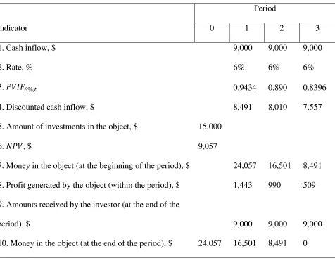
Table VI
Table 6. Economic interpretation of X
Indicator
Period
0 1 2 3
1. Сash inflow, $ 9,000 9,000 9,000
2. Rate, % 6% 6% 6%
3. &%, 0.9434 0.890 0.8396
4. Discounted cash inflow, $ 8,491 8,010 7,557
5. Amount of investments in the object, $ 15,000
6. , $ 9,057
7. Money in the object (at the beginning of the period), $ 24,057 16,501 8,491
8. Profit generated by the object (within the period), $ 1,443 990 509
9. Amounts received by the investor (at the end of the
period), $ 9,000 9,000 9,000
10. Money in the object (at the end of the period), $ 24,057 16,501 8,491 0
Since means increment, this indicator cannot be considered in isolation from the
amount of invested money ( ). However in calculating we don't take into account , and this
reduces the reliability of this indicator. Therefore, for reliable evaluation it is necessary to take
into account , invested money and a period of time. All these are combined in the "indicator
of the speed of specific increment in value" ( ) suggested by the author of the present paper:
S (13)
This indicator integrates two principles: "faster" and "more" and shows dollars of the
alternatives the one with the biggest indicator is the most cost-efficient. The strong point of is
that it is simple and realistic. This indicator does not require transforming cash flows. Let us use
to compare cars and . The owner's cash flows related to purchase and use of these cars are
given in tables 7 and 8.
[image:13.595.99.539.244.471.2]Table VII
Table 7. Owner's cash flows related to purchase and use of car
Indicator Period
0 1 2 3
1.Car price, $ 15,000
2.Car use income, $ 13,200 13,200 13,200
3.Operation costs, $ 5,000 5,000 5,000
4. A, $ -15,000 8,200 8,200 8,200
5. &%, 1 0.9434 0.890 0.8396
6.Discounted A, $ -15,000 7,736 7,298 6,885
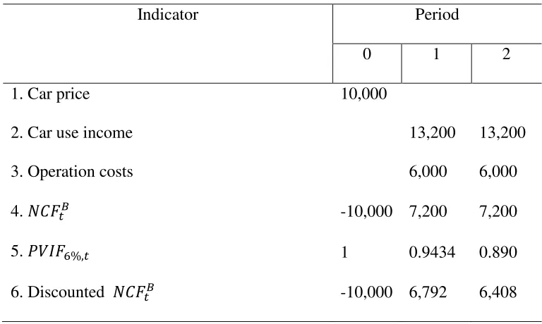
[image:13.595.126.510.551.781.2]Table VIII
Table 8. Owner's cash flows related to purchase and use of car
Indicator Period
0 1 2
1. Car price 10,000
2. Car use income 13,200 13,200
3. Operation costs 6,000 6,000
4. D -10,000 7,200 7,200
5. &%, 1 0.9434 0.890
and show that car is better: A= $6,919, D= $3,200; A =
$2,588; D = $1,746. However shows that car is better: A= 0.15 $/$ annually, D=
0.16 $/$ annually:
A $6,919
$15,000 3V2W/ 0.15$/$ 62/ V2W/ (14)
D $3,200
$10,000 2V2W/ 0.16$/$ 62/ V2W/ (15)
can be also applied in a reverse situation. Let us assume that an engineer has
developed a technical novelty which is an alternative to the existing equipment. The question is,
what maximum price it is possible to sell this novelty at? The maximum price of the novelty will
depend on the maximum the owner is ready to pay. It is he who will have to compare
"expensive, economic, long-term" equipment with "inexpensive, uneconomical, short-term".
This task can be solved in the following way. Let us assume that equipment with price
А and service life n exists, and alternative equipment with price В and service life m is
developed. These two alternatives have different production capacities and operation costs, and
thus different net cash flow: for equipment it is А, and for equipment this value will be
В. If we equate A to D, we get the following equation which is a basis for determining
characteristics of developed equipment:
∑ А
,
" ! А
S А
∑ В
,
" ! В
_ В (16)
On the basis of this equation we can determine boundary values of different characteristics
assume that A and В are annuities, in this case a condition for determining the
maximum price value of the developed equipment2 is obtained from the above equation:
В
` S
В
,5
_ А ,
А ! _ S
(17)
Let us use the above example to consider the operation of this formula. Assume that the
price of car is specified, and the maximum price of car is to be found. Using formula 17 and
data from tables 7 and 8, we obtain:
В 3V2W/ $7,200 3.465
2V2W/ $8,200 $15,000 ! 2V2W/ 3V2W/2.673 $10,096 (18)
If $10,096 is invested in car , its purchase efficiency will be equal to car purchase
efficiency:
D $3,104
$10,096 2V2W/ 0.15$/$ 62/ V2W/ (19)
If car sells at a higher price, it will be more cost-efficient for the owner to buy car .
So this paper discusses two indicators ( and ) which can help make a right
investment decision in a situation when different amounts for different periods of time are to be
invested in alternative real assets. The application range of these indicators is very wide: from a
small company buying an equipment unit to a state investing hundreds of billions of dollars. The
suggested and surely need a bit of criticism and if they stand up to it, we can consider
that the task of comparing this type of investments is solved.
2
Methods used to determine В and to take into account differences in production capacity of alternative
equipment types and differences in operation costs and prices are considered in the paper Коган А.Б. Способы
определенияэкономическиххарактеристикинноваций // Сибирскаяфинансоваяшкола. – №1. Новосибирск:
REFERENCES
Richard A. Brealey, Stewart C. Myers, 2003, Principles of corporate finance, Seventh Edition. The
McGraw-Hill Companies.
Richard A. Brealey, Stewart C. Myers, 2006, Principles of corporate finance, Eighth Edition.