http://www.scirp.org/journal/cweee ISSN Online: 2168-1570
ISSN Print: 2168-1562
Modeling of Unsteady Flow through Junction in
Rectangular Channels: Impact of Model
Junction in the Downstream Channel
Hydrograph
Seidou Kane
1*, Soussou Sambou
1, Issa Leye
1, Raymond Diedhiou
1, Seni Tamba
2,
Mouhamed Talla Cisse
2, Didier Maria Ndione
1, Mousse Landing Sane
11Faculty of Sciences and Technics, Department of Physics, Cheikh Anta Diop University, Dakar, Senegal 2Polytechnic High School of Thies, Thies, Senegal
Abstract
Open channel junctions are encountered in urban water treatment plants, ir-rigation and drainage canals, and natural river systems. Junctions are very important in municipal sewerage systems and river engineering. Adequate theoretical description of flow through an open channel junction is difficult because numerous variables are to be considered. Equations of junction mod-els are based on mass and momentum or mass and energy conservation. The objective of this study is to compare two junction models for subcritical flows. In channel branches, we solve numerically the Saint-Venant hyperbolic sys-tem by combining Preissmann scheme and double sweep method. We validate our results with HEC-RAS using Nash and Sutcliffe efficiency. In junction models, equality of water stage and complete energy conservation equation from HEC-RAS are compared. Outcome of the research clearly indicates that the complete conservation energy model is more suitable in flow through junction than equality of water stage model in serious situations.
Keywords
Junction Model, HEC RAS, Saint-Venant’s Equations, Double Sweep Method, Equality of Water Stages, Energy Conservation, Modelling of Flow
1. Introduction
Channel junctions are area of separation or meeting of natural or artificial flow networks. They are often encountered in open channel networks of drainage systems and river systems [1]. The efficiency of free surface drainage systems How to cite this paper: Kane, S., Sambou,
S., Leye, I., Diedhiou, R., Tamba, S., Cisse, M.T., Ndione, D.M. and Sane, M.L. (2017) Modeling of Unsteady Flow through Junction in Rectangular Channels: Impact of Model Junction in the Downstream Channel Hy-drograph. Computational Water, Energy, and Environmental Engineering, 6, 304-319. https://doi.org/10.4236/cweee.2017.63020
Received: May 7, 2017 Accepted: July 25, 2017 Published: July 28, 2017
Copyright © 2017 by authors and Scientific Research Publishing Inc. This work is licensed under the Creative Commons Attribution International License (CC BY 4.0).
http://creativecommons.org/licenses/by/4.0/
The objective of the present work is to show that the energy based junction model is generally more suitable than the equality of water stage junction model and should be applied in serious situations. We so compare the equality of water stage model, to the mass and energy model for a junction system. We calculate the external boundaries of the junction by solving Saint Venant’s equations us-ing Preissmann scheme for discretization and double sweep method for numer-ical solution along the channels of the network. Our calculations are validated by HEC-RAS software. Inputs of the network are simple and complex hydrographs. We then apply equality of water stage model to the junction. We then use HEC-RAS mass and energy based junction model for the same network with the same conditions. The two junction models are compared at the output of the network.
2. Materials and Methods
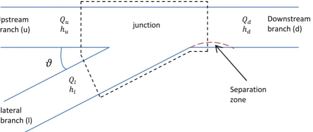
A junction system is composed by three channels at least: two upstream chan-nels and a downstream channel (Figure 1). Flow in the channels is simulated by solving numerically Saint-Venant’s equations. Two models can be used for inte-rior boundaries of the junction: mass and energy conservation method or mass and momentum conservation method. The first can be simplified to the equality of water stage model.
2.1. Numerical Solutions in Branches Using Double Sweep Method
The one-dimensional Saint-Venant equations are used to model transient open- channel flow for an incompressible homogeneous fluid. Saint-Venant model is a nonlinear hyperbolic system of two equations based on mass conservation and momentum conservation laws. The first (1a) is the continuity equation, and the second (1b) is the momentum equation.2
0 (1a)
0 (1b)
f
Q A
x t
Q Q Z
gA gAS
t x A x
∂ ∂
+ =
∂ ∂
∂ ∂ ∂
+ + + =
∂ ∂ ∂
(1)
[image:3.595.215.537.577.713.2]where Q = discharge; A = cross-sectional; g = acceleration due to gravity; Z =
elevation of the water surface, Sf= energy slope; t = temporal coordinate and x =
longitudinal coordinate. Complete Saint-Venant’s system is very popular among hydraulic engineers and hydrologists but have no analytical solutions so numer-ical solutions have been developed. Many numernumer-ical methods have been pro-posed for discretization: implicit or explicit [16]. Implicit scheme is very inter-esting because it is not subject to the Courant-Friedrichs-Levy stability condition
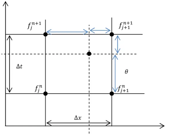
[17]. Among implicit schemes, the Preissmann one is the earliest used by hy-draulicians. It is a compact method using only four grid points for the solution and thus minimizes the damage done by the interpolated function. It was used in real situation and programmed with the details necessary to provide answers to real problems [18]. The generalized Preissmann scheme is presented in Figure 2. For a given space and time function f x t
( )
, , Preissmann scheme’sdiscretiza-tion is expressed as :
(
)
(
)
(
)
1 1
1 1 1 1 1
n n n n
j j j j
P
f =θ ϕ f++ + −ϕ f ++ −θ ϕ f + + −ϕ f (2)
(
1)
(
)
(
1)
1 1
1
1
n n n n
j j j j
P
f
f f f f
t t ϕ ϕ
+ +
+ +
∂ = − + − −
∂ ∆ (3)
(
1 1)
(
)
(
)
1 1
1
1
n n n n
j j j j
P
f
f f f f
x x θ θ
+ +
+ +
∂
= − + − −
∂ ∆ (4)
where j is the space index, n the time index and
θ
∈[ ]
0,1 ,ϕ
∈[ ]
0,1 areweighting coefficients. The Preissmann scheme is second-order accurate in both time and space if θ =0.5 and ϕ =0.5, and first-order accurate otherwise.
Li-near stability analysis shows that the centered scheme (ϕ =0.5) is
uncondition-ally stable for θ ≥0.5 [18].
[image:4.595.227.527.483.722.2]Introducing Equations (2), (3) and (4) in Equations (1a) and (1b), we obtain two nonlinear algebraic equations:
(
1 1)
(
)
(
)
(
1 1)
1 1 1 1
1
1 0
2
n n n n n n n n
j j j j j j j j
B
Q Q Q Q Z Z Z Z
x θ θ t
+ + + +
+ + + +
− + − − + − + − =
∆ ∆ (5)
(
)
(
)
(
)
(
)
(
)
(
)
(
)
(
)
( )
( )
1 1
2 2 2 2
1 1
1 1
1 1
1 1 1 1
1 1 1 1
1 1 1 1 1 2 1 1 1 2 1 2
n n n n
n n n n
j j j j
j j j j
n n n n n n n n
j j j j j j j j
n n
j j
Q Q Q Q
Q Q Q Q
t x S S S S
g
S S S S Z Z Z Z
x
g SJ SJ
θ θ
θ θ θ θ
θ + + + + + + + + + + + + + + + + + + − + − + − + − − ∆ ∆ + + + − + − + − − ∆
+
(
+ 1)
(
) ( )
(
( )
)
1
1 θ SJ nj SJ nj + + + − + (6)
The system is then linearized around an equilibrium steady-state by Taylor series expansion using Equations (7), (8) and (9):
1
n n
f f + f
∆ = − (7)
( ) ( )
2 1 2 2n n
f + − f ≅ f f∆ (8)
( )
20
f
∆ ≅ (9)
The following finite difference linear system is finally obtained:
11 1 12 1 11 12 13
21 1 22 1 21 22 23
(a) (b)
j j j j
j j j j
A Q A Z B Q B Z B
A Q A Z B Q B Z B
+ +
+ +
∆ + ∆ = ∆ + ∆ +
∆ + ∆ = ∆ + ∆ +
(10)
where A11, A12, B11, B12, B13, A21, A22, B21, B22 and B23 are
coeffi-cients resulting from the linearization. Equations (10a) and (10b) must be solved for all computational points for every time step during the period of computa-tion and any standard resolucomputa-tion method can be applied if the boundary condi-tions are also linearized. They are written for every reach connecting two nodes on the computational domain. Thus for a domain of N computational points there are 2N-2 discretized equations. Since there are two unknowns at each node, there are 2N unknowns in the domain, so two boundary conditions are needed to close the system [19].
In this paper, we use the double sweep method as applied by Preissmann and Cunge. The number of elementary operations necessary to solve the system by this method is proportional to the number of points N while standard methods of matrix inversion is proportional to 3
N . A short presentation is described
be-low:
The rating curve Q Z
( )
is generally non linear. But locally, around a spatialpoint j, ∆Qj and ∆Zj can be considered enough small to assume there a
linear relationship of the type of Equation (11) [18][20]:
j j j j
Q E Z F
∆ = ∆ + (11)
We eliminate ∆Qj in the Equations (10a) and (10b) by multiplying the first
equation by B21, the second by −B11 and we obtain the Equation (12):
(
)
(
)
(
)
11 21 21 11 1 12 21 22 11 1
12 21 22 11 13 21 23 11
j j
j
A B A B Q A B A B Z
B B B B Z B B B B
+ +
− ∆ + − ∆
= − ∆ + − (12)
1 1
j j j j j j
Z L Q+ M Z + N
∆ = ∆ + ∆ + (13)
where:
(
)
(
1211 2121 2122 1111)
j
A B A B
L
B B B B
− =
− (14)
(
)
(
1212 2121 2222 1111)
j
A B A B
M
B B B B
− =
− (15)
(
)
(
1223 1121 1322 2111)
j
B B B B
N
B B B B
− =
− (16)
Substitution of Equation (11) into Equation (10a) leads to:
(
)
11 j1 12 j1 12 11 j j 11 j 13
A ∆Q+ +A ∆Z + = B +B E ∆ +Z B F +B (17)
Then replacing ∆Zj in Equation (17) by its value in (13), we obtain Equation
(18):
(
)(
)
11 j1 12 j1 12 11 j j j1 j j1 j 11 j 13
A ∆Q+ +A ∆Z + = B +B E L∆Q+ +M ∆Z + +N +B F +B (18)
Rearranging Equation (18) finally leads to:
1 1 1 1
j j j j
Q+ E+ Z + F+
∆ = ∆ + (19)
where:
(
)
(
)
12 11 12
1
11 12 11
j j
j
j j
M B B E A
E
A L B B E
+
+ −
=
− + (20)
(
)
(
)
12 11 11 13
1
11 12 11
j j j
j
j j
N B B E B F B
F
A L B B E
+
+ + +
=
− + (21)
Equation (19) represents the recurrence relation at point j+1. The
coeffi-cients Ej+1 and Fj+1 can be known for any point j+1 if the analogous
coef-ficients Ej and Fj are known at the previous point j.
We start the calculations from the upstream by setting the hydrograph Q(t) for j=1. According to Equation (11), coefficient E1 should be equal to zero
because ∆Q1 is independent of ∆Z1, so: 1 0
E = and F1= ∆Q1
At the downstream boundary ( j=N), ∆ZN should be known. We retained
a uniform flow rating curve. In this case using Manning-Strickler’s law we can compute ∆ZN and ∆QN by:
( )
( )
N N N
N N
Q Z F Q
Z Q Z E Z − − ∆ = ∂ − ∂ (22)
N N N N
Q E Z F
∆ = ∆ + (23)
appropri-ate formulation to take into account the complexity of free surface flow. The HEC-RAS software solves the one dimensional unsteady flow equations by writ-ing Saint-Venant equations in a general formulation for 1D flow in flood plain as follow [21]:
(
)
(
1)
0
c f
Q Q
A
t x x
∂ − Φ ∂ Φ
∂
+ + =
∂ ∂ ∂ (24)
(
2 2)
(
1 2)
20
f c
c fc f ff
c f c f
Q A
Q A
Q z z
gA S gA S
t x x x x
∂ − Φ
∂ Φ
∂ ∂ ∂
+ + + + + + =
∂ ∂ ∂ ∂ ∂ (25)
Subscripts (c) is associated to channel and (f) to floodplain, Q is the total
flow, Φ is a coefficient, K is the conveyance.
In our application the channels are rectangular and there is no flow over the banks. Thus the system of equations used by Hec-Ras becomes the same as the system of Equations (1a), (1b) described previously.
Numerical solution program of Saint-Venant used in HEC-RAS is based on the U.S. Army Corp of Engineer’s (USACE) model Unsteady Network Model. This program solves the mass conservation and momentum conservation equa-tions with an implicit linearized system of equaequa-tions using Preissman’s second order box scheme. The simultaneous system of equations generated for each time step (and iterations within a time step) are stored with a skyline matrix scheme and reduced with a direct solver developed specifically for unsteady river hydraulics by Dr. Robert Barkau. The state variables for the numerical scheme are flow and stage, which are computed and stored at each cross section. The hydraulic resistance is based on the friction slope from the empirical Manning’s equation, with several ways of modifying the roughness. Roughness can be cha-racterized with Manning’s (n) or roughness height’s (k) (William E. F. 2003).
2.3. Junction Models
Numerical models junction in open channel networks are based on the mass conservation associated either to the energy conservation or to the momentum conservation [4][7].
2.3.1. Hec-Ras Junction Model
2 2
2 2 1 1
02 2 01 1
2 2 e
V V
Z Y Z Y h
g g
α α
+ + = + + + (26)
where: Z0j = elevation of the main channel invert at cross section j; j
Y = depth of water at cross section j;
j
V = average velocity cross section j; he = energy head loss; j
α
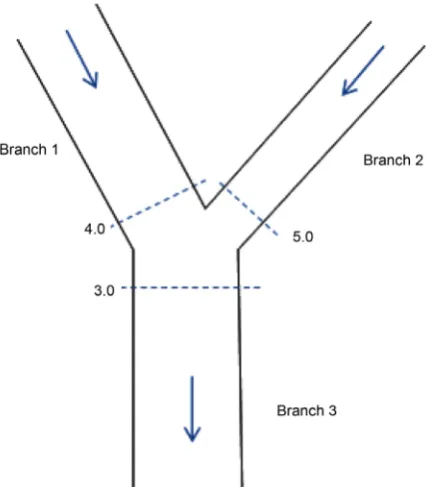
= velocity weighting coefficient at cross section j.Subcritical flow calculations are performed up to the most upstream section of branch 3. The water surface at branch 1 is calculated by performing a balance of energy from station 3.0 to station 4.0. Friction losses are based on the length from station 4.0 to 3.0 and the average friction slope between the two sections (Figure 3). Contraction and expansion losses are also evaluated across the junc-tion. The energy equation from station 3.0 to 4.0 is written as follows [21]:
2 2
2 2
3 3 3 3
4 4 4 4
04 4 03 3 4 3 4 3
2 2 f 2 2
V V
V V
Z Y Z Y L S C
g g g g
α
α
α
α
→ →
+ + = + + + + − (27)
The water surface for the downstream end of branch 2 is calculated in the same manner.
2.3.2. Equality of Water Surface Model
[image:8.595.267.481.469.713.2]Energy losses and differences in velocity head are difficult to evaluate, so that the interior boundary conditions may simply diminish to the equality of water sur-face elevations (Equation (28)) associated to the macroscopic version of conti-nuity equation (Equation (29)), as in many software such as the One Dimen-sional Hydrodynamic Model Environment Canada 1988; Mike 11 model Danish Hydraulic Institute 1999; and Chaudhry 1993. The equations of the model are written as follows:
04 4 03 3 05 5
Z +Y =Z +Y =Z +Y (28)
3 4 5
Q =Q +Q (29)
3. Applications and Results
3.1. Characteristics of the Hydraulic System
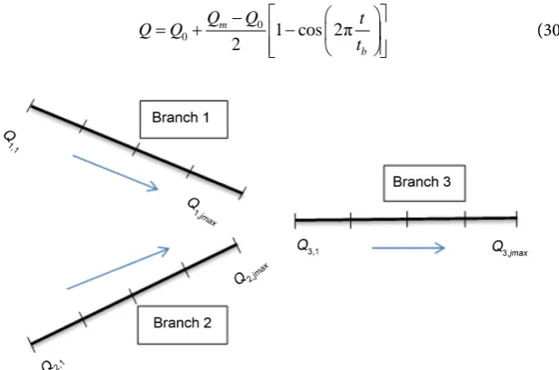
The network is represented by three identical rectangular branches related by a junction (Figure 4).
The geometric and hydraulic characteristics of the system are given in Table 1
(length, width, slope, and roughness). The numerical parameters (space step, time step, weighting coefficient) used in the double sweep method and in Hec- Ras software are presented in Table 2.
• Upstream boundary conditions
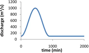
At the input of the upstream branches constituting the junction, we chose a simple Henderson sinusoidal hydrograph (HS, Equation (30)), a two complex Henderson hydrographs, one with two equal peaks (HC2, Equation (31)), and another with three decreasing peaks (HC3D, Equation (32)). The corresponding hydrographs are shown in Figures 5-7.
0
0 1 cos 2π
2
m
b
Q Q t
Q Q
t
−
= + −
[image:9.595.226.534.340.544.2] (30)
[image:9.595.206.539.600.668.2]Figure 4. Hydraulic system.
Table 1. Characteristics of the network system.
Branch Length (m) Width (m) Ks Slope I
B1 150,000 120 50 0.0001
B2 150,000 120 50 0.0001
B3 150,000 120 50 0.0001
Table 2. Numerical parameters.
x
∆ (m) ∆t (s) Θ
Figure 5. Simple henderson hydrograph (HS).
Figure 6. Complex henderson hydrograph (HC2).
Figure 7. Complex henderson hydrograph (HC3D).
with
3
peak flow 1000 m s
m
Q = =
3 0 initial flow 100 m s
Q = =
base time 10 h
b
t = =
0
1 0
0 2
1 2
1 cos 2π 2
1 cos 2π 2 , , p b b p b b
Q Q t
Q Q t t
t
Q Q t d
Q d t t d
t
Q Q Q
− = − + ≤ − −
= − < ≤ +
= + (31) 0 200 400 600 800 1000 1200
0 1000 2000
di sc ha rg e ( m 3/s) time (min) 0 100 200 300 400 500 600
0 500 1000 1500 2000
di sc ha rg e( m 3/s) time (min) 0 200 400 600 800 1000 1200 1400
0 1000 2000 3000
[image:10.595.266.479.386.513.2]3 3 0
,
500 m s 100 m s
p
Q = Q =
15 h and 13 h
b
t = d=
0 1 0 0 2 0 3
1 2 3
1 cos 2π , 2
1 cos 2π , 1.5
2
1 cos 2π , 2 2
1 p b b p b b p b b
Q Q t
Q Q t t
t
Q Q t d
Q d t t d
t
Q Q t d
Q d t t d
t
Q Q Q Q
− = + − ≤ − −
= − < ≤ +
− −
= − < ≤ +
= + + (32) 3 3 0 ,
400 m s 100 m s
p
Q = Q =
15 h, 13 h
b
t = d=
• Downstream boundary conditions.
For downstream boundary conditions we have chosen a steady-state calibra-tion curve:
( )
23 12s H
Q Z =K ⋅ ⋅S R ⋅I (33)
s
K = Manning’s coefficient; RH = hydraulic radius; I = slope of the
channel.
• Initial condition is set by using a uniform flow with 3 0 100 m s. Q =
3.2. Criteria for Comparison
Hydrographs calculated according to our program are compared to those given by HEC RAS package. Two kind criteria are used for comparison: local criteria (Relative Peak Error or RPE, Equation (34); Relative Volume Error or RVE, Eq-uation (35)) and global statistical criteria (Nash-Sutcliffe coefficient, EqEq-uation (36)).
mHec mDS mHec
RPE Q Q
Q −
= (34)
Hec DS Hec
RVE V V
V −
= (35)
(
)
(
)
2 0 1 2 0 0 1 NASH 1T t t
m t T t t Q Q Q Q = = − = − −
∑
∑
(36)where QmHec is the maximum discharge calculated by Hec-Ras; QmDS is the
maximum discharge calculated with our program; VHec is the volume by Hec-
Ras; VDS is the volume by our program; 0
t
Q is discharge at time t, Q0, are
respectively and the mean of discharges calculated by Hec-Ras. t m
Q is the
computation are equal. A NASH criterion close to 1 means a good representa-tion of the hydrograph calculated by our program compared to that computed with HEC RAS.
4. Results and Discussions
There are two main characteristics of flow motion in channels: translation and attenuation. In translation, shape of the hydrograph is maintained along the channel while attenuation involves the reduction of the peak flow and the change of the shape of the hydrograph. Translation is dominant in steep straight channel, and attenuation is channel with storage. The downstream hydrographs are compared here.
We first validate our program in a single branch and then introduce the junc-tion model.
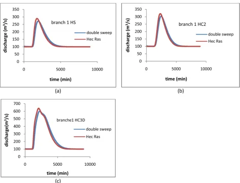
• Flow in a single branch (B1): model validation
[image:12.595.60.534.354.715.2]We first compared downstream hydrographs of branch 1 that we have calcu-lated to that computed with HEC-RAS. Corresponding results are presented in
Figure 8. Criteria are presented in Table 3.
According to Table 3, RPE and RVE are very small, while Nash criterion is
close to unity. This shows that our program reproduces well the flow in the channel compared to Hec-Ras model for simple and complex upstream hydro-graphs (Figure 8). It also lightly underestimates the peak flow while the volume of flow is almost the same. When we have a complex upstream hydrograph (Figure 6 and Figure 7) we obtain a simple hydrograph at the downstream end of the hydraulic system (Figure 8(b) and Figure 8(c)), this is due to the length of the branch. The channels of the system are very long so diffusion and also at-tenuation have to be more important and that makes the other peaks disappear.
• Flow through the whole network with Junction models
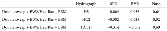
We have then compared the hydrographs downstream the junction computed with the water surface equality method (EWS) to that of Hec-Ras junction me-thod (EBM). Figure 9 shows the resulting hydrographs, and Table 4 the local and global characteristics.
Figure 9 shows a net difference between the hydrographs downstream of the
Table 3. Local and global characteristics in single branch B1.
Hydrograph RPE RVE Nash
Double sweep/Hec-Ras HS 0.058 −0.003 0.93
Double sweep/Hec-Ras HC2 0.046 −0.003 0.95
Double sweep/Hec-Ras HC3D 0.059 −0.001 0.95
Table 4. Local and global characteristics after the junction (branch 3).
Hydrograph RPE RVE Nash
Double sweep + EWS/Hec-Ras + EBM HS −0.064 0.056 0.64
Double sweep + EWS/Hec-Ras + EBM HC2 −0.302 0.028 0.52
Double sweep + EWS/Hec-Ras + EBM HC3D −0.314 −0.002 0.69
junction obtained with the equality of the water surface (EWS) and that obtained by the energy based model (EBM): EWS junction model overestimates the peak flow and decreases the falling limb’s times of hydrographs when compared to EBM based model. We can see in Table 4 that RPE is negative and significant, the volume is slightly the same for the two approaches, and Nash criterion is rel-atively small but not very close to unity.
According to Figure 9, translation effect is more important in EWS model, while natural attenuation of hydrograph downstream the junction is well repro-duced with EBM (HEC RAS). A theoretical justification of this fact is underta-ken by comparing Equation (26) for EBM and (28) for EWS: it appears that the main difference in the pattern of hydrographs downstream of the junction be-tween EWS and EBM model is due to the kinetic and friction losses terms at the junction. These terms are precisely those that lead to the attenuation of natural hydrograph observed during the propagation of the flood wave. It is obvious that neglecting these two terms impacts the shape of the hydrograph downstream the junction. This shows that EWS model is less suitable than EBM for junction. Simplified methods generally don’t have the accuracy of a solution procedure based on the complete equation. They can give sufficiently accurate results when all the assumptions are well defined and respected.
5. Conclusion
conclusion, although much easier to implement, the junction model based on the equality of water surface is less suitable in channel network.
References
[1] Wu, R. and Mao, Z.Y. (2003) Numerical Simulation of Open Channel Flow in 90- Degree Combining Junction. Tsighua Science and Technology, 8, 713-718.
[2] Pfister, M., Gokkok, T. and Gisonni, C. (2013) Les jonctions avec les écoulements torrentiels. Séminaire VSA/EPFL Hydraulique des canalisations, Lausanne.
[3] Baghlani, A. and Talebbeydokhti, N. (2013) Hydrodynamics of Right-Angled Channel Confluences by a 2D Numerical Model. IJST, Transactions of Civil Engi-neering, 37, 271-283.
[4] Shabayek, S., Stiffler, P. and Hicks, F. (2002) Dynamic Model for Subcritical Com-bining Flows in Channel Junctions. Journal of Hydraulic Engineering, 128, 821-828.
https://doi.org/10.1061/(ASCE)0733-9429(2002)128:9(821)
[5] Hsu, C.C., Lee, W.J. and Chang, C.H. (1998) Subcritical Open Channel Junction Flow. Journal of Hydraulic Engineering, 124, 847-855.
https://doi.org/10.1061/(ASCE)0733-9429(1998)124:8(847)
[6] Bowers, C.E. (1950) Hydraulic Model Studies for Whiting Field Naval Air Station. Part V. Studies of Open-Channel Junctions. Saint Anthony Falls Hydraulic Labora-tory Project Report No. 24.
[7] Vasquez, J., Ghenaim, A., Ghostine, R., Kesserwani, G. and Mose, R. (2007) Simula-tion of Subcritical Flow at a Combining JuncSimula-tion. NOVATECH, 497-504.
[8] Sivakumar, M., Dissanayake, K. and Godbole, A. (2004) Numerical Modeling of Flow at an Open-Channel Confluence. In: Mowlei, M., Rose, A. and Lamborn, J., Eds., Environmental Sustainability through Multidisciplinary Integration, Environ- mental Engineering Research Event, Australia, 97-106.
[9] Brito, M., Canelas, O.B., Leal, J.L. and Cardoso, A.H. (2014) 3D Numerical Simu- lation of Flow at a 70˚ Open-Channel Confluence. V Conferência Nacional de Mecânica dos Fluidos, Termodinâmica e Energia MEFTE 2014, Porto, Portugal APMTAC, 11-12 Setembro 2014.
[10] Longxi, H. (2008). Parameter Estimation in Channel Network Flow Simulation.
Water Science and Engineering, 1, 10-17.
https://doi.org/10.1016/S1674-2370(15)30014-4
[11] Ewemoje, T.A. and Abimbola, O.P. (2014) Verification of Coefficient of Rectangu- lar Side Weirs Using Shabayek Model. Research Journal of Applied Sciences, 9, 397- 401.
[12] Sharkey, J.K. (2014) Investigating Instabilities with HEC-RAS. Unsteady Flow Mod-eling for Regulated Rivers at Low Flow Stages. Master Thesis, University of Tennes-see, Knoxville.
[13] Chandresh, G.P. and Gundaliya, P.J. (2016) Floodplain Delineation Using HECRAS Model—A Case Study of Surat City. Open Journal of Modern Hydrology, 6, 34-42.
https://doi.org/10.4236/ojmh.2016.61004
[14] Direction Departementale de L’equipement et de L’agriculture (DDE 42) (2010) Etude hydraulique de la rivière le gier et de ses affluents. Rapport d’étude hydraulique. Sogreah JCC/JMI 1741145 R2 MAI.
[15] Smival (2011) Etude hydraulique de la Lèze: Simulation des crues synthétiques. [16] Fread, D.L. and Jin, M. (1997) Dynamic Flood Routing with Explicit and Implicit
https://doi.org/10.1061/(ASCE)0733-9429(1997)123:3(166)
[17] Litrico, X., Pomet, J.B. and Guinot, V. (2010) Simplified Nonlinear Modeling of Ri- ver Flow Routing. Advances in Water Resources, 33, 1015-1023.
[18] Cunge, J.A. and Liggett, J.A. (1975) Unsteady Flow in Open Channels. Water Re- sources Publications. In: Mahmood, K. and Yevjevich, V., Eds., Chapter 4, Nume- rical Methods of Unsteady Flow Equations, Colorado, 89-182.
[19] Meselhe, E.A. and Holly, F.M. (1997) Invalidity of Preissmann Scheme for Transcri- tical Flow. Journal of Hydraulic Engineering, 123.
https://doi.org/10.1061/(ASCE)0733-9429(1997)123:7(652)
[20] Preissmann, A. (1961) Propagation des intumescences dans les canaux et rivières.
First Congress of the French Association for Computation, Grenoble, 433-442. [21] US Army Corp of Engineers Institute for Water Resources (2010) HEC-RAS River
Analysis System Hydraulic Reference Manual Version 4.1. Davis.
Submit or recommend next manuscript to SCIRP and we will provide best service for you:
Accepting pre-submission inquiries through Email, Facebook, LinkedIn, Twitter, etc. A wide selection of journals (inclusive of 9 subjects, more than 200 journals)
Providing 24-hour high-quality service User-friendly online submission system Fair and swift peer-review system
Efficient typesetting and proofreading procedure
Display of the result of downloads and visits, as well as the number of cited articles Maximum dissemination of your research work
Submit your manuscript at: http://papersubmission.scirp.org/