Does the Biased Coefficient Problem Plague the VAR Model?

ISSN Online: 2162-2086 ISSN Print: 2162-2078

DOI: 10.4236/tel.2017.73034 April 13, 2017

Does the Biased Coefficient Problem Plague the

VAR Model?

Yunyun Lv

Department of Economics, Kansas State University, Manhattan, KS, USA

Abstract

This paper documents evidence to investigate if the explanatory variables are always correlated with the error term in the vector autoregression (VAR) model because of the property of the VAR model. I use Christiano et al. (CEE, 2005) as an example to examine this argument empirically. According to the findings of this paper, the impulse responses provided by the structural VAR model may be derived from the biased estimates if we allow variables to be correlated with each other through different horizons. It remains possible for a skeptic to maintain some dominant views inferred from the biased coeffi-cients of the SVAR models.

Keywords

Impulse Response Functions, The Biased Estimated Coefficients

1. Introduction

Since Sims (1980) [1], the vector autoregression (VAR) model becomes a useful tool to make out-of-sample forecasts in macroeconomics, especially forecasting how the variables are going to change after a shock by adding restrictions to the VAR model, holding all other shocks constant. However, a lot of plausible and contrary results of the structural vector autoregression (SVAR) models exist in the literature. Bernanke et al. (1997) [2] test the hypothesis that the response of monetary policy to oil shocks causes recessions by BGW model. Hamilton and Herrera (2004) [3] demonstrate that when more lags of variables are modeled, monetary policy is far less powerful. Moreover, Hamilton (1983) [4] suggests a significantly negative correlation between oil prices and output during some of the recessions before 1972. Hooker (1996) [5] provides evidence that the correla-tion between oil prices and economic activity becomes much weaker since 1985. The instability of the empirical relations among variables in the literature may be

How to cite this paper: Lv, Y.Y. (2017) Does the Biased Coefficient Problem

Pla-gue the VAR Model? Theoretical

Econom-ics Letters, 7, 454-463.

https://doi.org/10.4236/tel.2017.73034

Received: February 27, 2017 Accepted: April 10, 2017 Published: April 13, 2017

Copyright © 2017 by author and Scientific Research Publishing Inc. This work is licensed under the Creative Commons Attribution International License (CC BY 4.0).

http://creativecommons.org/licenses/by/4.0/

attributed to the biased estimated coefficients of the SVAR models.

This paper demonstrates a weakness of current empirical practice in the VAR literature: I try to check if the estimated error term is always correlated with the lagged variables on the right-hand side (R.H.S.) of the VAR model because of the structure of the VAR model, which is an analogous question of the correlations between the identified shocks and the explanatory variables in the structural vector autoregression (SVAR) model. If the above correlations exist, it indicates that the estimated coefficients of the VAR model are biased.

Likewise, Friedman (1961) [6] advocates that for the eighteen non-war busi-ness cycles since 1870, monetary policy affects economic conditions only after a lag which is long and variable. Blanchard and Quah (1989) [7] appeals to an analogous argument regarding that some variables are more important at some horizons than at others. They point out that demand disturbances have a hump-shaped effect on output, which disappears after about two years, while supply disturbances have a continually increasing effect on the output which reaching a plateau after five years.

Lv (2017) [8] provides a new assumption that different variables may affect the economy through different horizons. The impulse-response function (IRF) usually employs the same variables selected one-step ahead for multi-step ana-lyses. When a one-step-ahead structural VAR model is used for all horizons, the fluctuations of the variables selected one-step ahead may affect some omitted va-riables which are not in this model, then those omitted vava-riables may affect the variables in the system significantly over long horizons. From the findings of Lv (2017) [9], the contributions of the omitted variables may be taken by the va-riables in the SVAR model under the new assumption, so the traditional impulse response results may not be credible since they ignore the significant effects of these important omitted variables through a long-horizon perspective.

The innovation of this paper is that under the new assumption that variables may vary over different horizons, I test if the variables may be correlated with the error terms in the VAR model through a long-horizon perspective. To my knowledge, this is the first paper to check the biased coefficient problem of the VAR model. This paper contributes to the literature by questioning the reliabili-ty of the impulses response results derived from the existing SVAR models. When talks about the ceteris paribus, if outside variables will not change, the es-timated coefficients of variables in the SVAR models are actually overeses-timated. I provide convincing evidence that the error term may be always correlated with variables on the R.H.S. of a VAR model through different horizons.

The paper is organized as follows. Section 2 interprets the relations between the identified shocks and the lags of variables on the R.H.S. of the SVAR model. Section 3 uses an existing SVAR model to gauge the biased coefficient problem empirically. Concluding comments are given in Section 4.

2. Interpretation

equ-456

ations are not misspecified and the residuals are not autocorrelated. However, if we include more lags in the model, these lags may be correlated with the error term. In this paper, since all variables in the SVAR system are considered as the combinations of shocks, I try to check if the estimated coefficients of the SVAR model are biased.

In detail, a standard SVAR model is usually given by:

(

)

1 1 2

0 0

1

, 0,

p

t i t i t t

i

y A A y− − A u u− N σ

=

=

∑

where yt is a vector of the model variables, P is the lag length of the

va-riables in the system and ut is the vector of structural shocks. Ai denotes the

matrices of parameters corresponding to the ith lag and I have left out the vec-tor of constant terms to keep things simple. According to the suggestion in Sims (1980) [1], the Cholesky decomposition which requires that 1

0

A− be lower trian-gular is usually used as restrictions. This structure indicates that the variable listed at the top of yt affects the remaining variables contemporaneously, while the

second variable from the top has immediate causal effects on all the variables except the first and so on down the list. We can also write it in the form of Equation (2):

(

)

0

1

t t

y = +βL+ + β+∞ +∞L A u−

Equation (2) shows that variables are the combinations of the shocks. We can also transfer Equations (2)-(4) to make the above argument clear.

(

)

1 1 0 1

t t

y₋ = +βL+ + β+∞ +∞L A u− ₋

(

)

1 0

t t

y₋ = L+βL + + β+∞ +∞L A u− (4)

According to Equations (1)-(4), yt and yt−1 are both correlated with ut,

which implies that the lags of the variables on the R.H.S. of the SVAR model may be correlated with the error term through longer horizons and motivates us to wonder how reliable its impulse response results are.

Likewise, Lv (2017a) [9] postulates that the estimated coefficients may be bi-ased if the variables affect the economy through various time spans. To exempl-ify, I assume that one more type of shocks affect GDP in y significantly after a year for quarterly data in Equation (5):

(

)

GDP_t = L +δL + + δ+∞ +∞L _t (5)

It is possible that the shocks selected one-step ahead in ut may take the

con-tributions of the omitted shocks t as their own. The traditional IRFs assume

that these exogenous structural innovations are independent and identically dis-tributed random variables. The policy intuition behind this paper is that the fluctuations of economic time series may not be from random shocks, these in-novations may be correlated with each other or the variables through different horizons.

3. Empirical Analysis

457

which is often used in estimating the multi-step response of one variable to an impulse in another variable in a system, has been widely used in many articles. In this section, I use the SVAR model in Christiano et al. (CEE, 2005) [10] as an example.

Christiano, Eichenbaum, and Evans construct a model with a moderate degree of nominal rigidities that prevents a sharp rise in marginal costs, generating in-ertial inflation and persistent output movements after an expansionary shock to monetary policy.

The form of the CEE model is as follows:

(

)

1

, 0,

p

t i t i t t i

F B F− Cu u N σ

=

=

∑

t

F contains nine quarterly series. The lag length p of the model is set to 4. The order of variables is the real gross domestic product (GDP), the real consumption (RPCE), the GDP deflator (GDPDEF), real investment (INVEST), the real wage (WAGE), labor productivity (PROD), the federal funds rate (FEDFUNDS), real profits (PROFIT) and the growth rate of M2 (M2).

The matrix C is taken to be lower triangular with ones along the principal di-agonal. It implies that the variables except real profits and the M2 growth rate will not respond instantaneously to monetary policy innovations.

All estimates reported in this paper are based on the original dataset from 1965Q3-1995Q2 in CEE (2005) [10]1_{. All data can also be downloaded from}

Federal Reserve Economic Data (FRED) provided by the Federal Reserve Bank of St. Louis. The real GDP, the real consumption, real investment, the real wage, labor productivity, and real profits are measured as 100 times the natural loga-rithm of the original data. The federal funds rate is expressed as annualized per-centage points. Inflation is 100 times the natural logarithm of the ratio of the in-dexes for CPIt and CPIt−1. Money growth of M2 are the first difference of 100 times the natural logarithm of the original data. The first eight transformed va-riables are still not stationary, I use the first difference of these vava-riables, and leave the money growth of M2 alone.

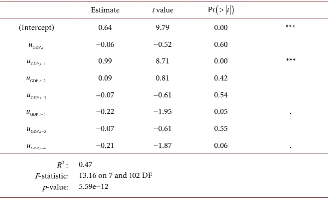
I begin by checking if the estimated error term is correlated with the first lag of the real output on the R.H.S. of the CEE model in Equation (7). I regress the real output at time t−1 on the output shocks and the lags of the output shocks

estimated from the CEE model.

6

1 0 GDP,

0

GDPt i t p t

i

u

α β ε

− −

=

= +

∑

Table 1 presents the regression estimation of Equation (7)2_{, which shows the}

effect of an output shock on output over different horizons. The coefficient es-timates, t-statistics, and p-values are reported in column 2-4, with the level of significance of the coefficients appearing on the right side of p-values. In this re-search, I use *** to denote 0.1% level of significance of the coefficients; **, de-noted as 1% significance; *, as 5% significance; ., as 10% significance. The 0.1%

1_{The data are provided by Martin Eichenbaum.}

458

level of significance implies that there is about 1 in 1000 chance that a significant result is actually due to chance.

Based on the findings of Table 1, the estimated coefficients of the lags of the real output shocks can be statistically significant at 0.1% level.

Then I check if the first lag of the real consumption listed second in the CEE model is correlated with the real output shocks:

6

1 0 GDP,

0

RPCEt i t p t

i

u

α β ε

− −

=

= +

∑

Table 2 shows parameter estimates of Equation (8). The coefficients of the real output shocks at time t−1 and t−5 are statistically significant at the 1%

and 5% level, respectively. Again, I find that the relation between the lags of the output shocks and the explanatory variables on the R.H.S. of the CEE model ex-ists, which indicates that the error term are correlated with the variables in the

Table 1. The regression estimation of the first lag of GDP on the GDP innovations.

Estimate t value Pr

( )

(Intercept) 0.64 9.79 0.00 ***

GDP,t

u −0.06 −0.52 0.60

GDP,t1

u − 0.99 8.71 0.00 ***

GDP,t2

u − 0.09 0.81 0.42

GDP,t3

u − −0.07 −0.61 0.54

GDP,t4

u − −0.22 −1.95 0.05 .

GDP,t5

u − −0.07 −0.61 0.55

GDP,t6

u − −0.21 −1.87 0.06 .

2 R :

F-statistic: p-value:

0.47

13.16 on 7 and 102 DF 5.59e−12

Table 2. The regression estimation of the first lag of the real consumptions on the real

GDP innovations.

Estimate t value Pr

( )

(Intercept) 0.35 8.40 0.00 ***

GDP,t

u −0.02 −0.31 0.75

GDP,t1

u − 0.25 3.34 0.001 **

GDP,t2

u − −0.04 −0.58 0.56

GDP,t3

u − −0.08 −1.05 0.30

GDP,t4

u − 0.07 0.90 0.37

GDP,t5

u − −0.18 −2.42 0.02 *

GDP,t6

u − −0.12 −1.57 0.12

2 R :

F-statistic: p-value:

0.19

system through different horizons and the estimated coefficients may be biased. In Equation (9), I demonstrate the impact of the output shocks on the first lag of each variable on the R.H.S. of the CEE model.

6

1 0 GDP,

0

t i t p t

i

Y− α βu − ε

=

= +

∑

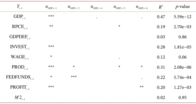
Table 3 presents the regression results of the empirical models represented by Equation (8). The first two rows display the significance level of coefficients in Equation (7) and Equation (8), respectively. Since the estimated coefficients of the output shocks at time t and t−3 are not significant for all variables, I drop

them from Table 3 for simplifications. Column 1 lists the dependent variable

1

t

Y− in Equation (9). Columns 2 to 7 are the significance level of the estimated coefficients of the lags of output shocks. The 2

R and the p-value of the equa-tion on the first row are shown in Columns 8 and 9, respectively.

According to the outcomes of Table 3, the first lag of the output shocks is correlated with the first lag of all variables except the GDP deflator and M2. If more lags of the output shocks are included in the equations, even the first lag of the GDP deflator and M2 may be correlated with output shocks significantly through longer horizons. The equations except the real consumption, the GDP deflator, the real wage and M2 have 2

R greater than 20% and the p-value less than 0.05. It is reasonable for us to conclude that these lags of the output shocks impact most of the variables through longer horizons in the CEE model.

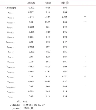
Since I find that the first lag of the GDP deflator and M2 are not correlated with the first sixth lags of the output shocks, then I regress them on the other kinds of shocks in Equation (10), respectively:

2 2

1 0 GDP, GDP, 2, 2,

1 1

t i t p M i M t p t

i i

Y− α β u − β u − ε

= =

= +

∑

∑

Table 4 displays the estimates of the effect of the first two lags of all shocks on the GDP deflator at time t−1 on the R.H.S. of the CEE model. The regression

has an 2

R of 75%. If the lags of these shocks do not impact the GDP deflator,

Table 3. Statistical significance of the real output shocks for each variable in the CEE

model.

1

t

Y− uGDP,t−1 uGDP,t−2 uGDP,t−4 uGDP,t−5 uGDP,t−6 R2 p-value

1

GDPt− *** . . 0.47 5.59e−12

1

RPCEt− ** * 0.19 2.70e−03

1

GDPDEFt− 0.03 0.86

1

INVESTt− *** 0.28 1.81e−05

1

WAGEt− * . 0.12 0.06

1

PRODt− *** * * * 0.31 2.08e−06

1

FEDFUNDSt− * *** . 0.22 5.74e−04

1

PROFITt− *** ** 0.20 1.27e−03

1

2t

460

Table 4. Estimation of the regression of the first lag of the GDP deflator on lags of all

in-novations.

Estimate t value Pr

( )

(Intercept) −0.002 −0.08 0.94

GDP,t1

u − 0.007 0.18 0.86

RPCE,t1

u − −0.19 −2.75 0.007 **

GDPDEF,t1

u − 0.99 13.05 0.00 ***

INVEST ,t1

u − 0.0002 0.01 0.99

WAGE,t1

u − −0.005 −0.05 0.96

PROD,t1

u − 0.005 0.10 0.92

FEDFUNDS,t1

u − 0.02 0.72 0.47

PROFIT ,t1

u − 0.0004 0.07 0.94

2, 1

M t

u − −0.009 −0.17 0.86

GDP,t2

u − 0.09 2.20 0.03 *

RPCE ,t2

u − 0.18 2.61 0.01 *

GDPDEF,t2

u − −0.62 −8.20 0.00 ***

INVEST ,t2

u − −0.04 −1.83 0.07 .

WAGE ,t2

u − 0.29 3.25 0.002 **

PROD,t2

u − −0.05 −0.90 0.37

FEDFUNDS,t2

u − 0.06 2.03 0.05 *

PROFIT ,t2

u − 0.009 1.45 0.15

2, 2

M t

u − 0.06 1.13 0.26

2 R :

F-statistic: p-value:

0.75

15.89 on 7 and 102 DF <2.20e−16

the 2

R for this regression should be approximately zero. The coefficients of all shocks except uPROD, uPROFIT and uM2 are significant. The estimated coeffi-cients of uGDP,t−2 uRPCE,t−2 and uGDPDEF,t−2 are significant, indicating that the GDP deflator is correlated with the sum of these shocks through different hori-zons, so the estimated coefficients of the GDP deflator equation in the CEE model may be biased.

The interesting part is that the estimated coefficients of uGDP,t−1 is not signif-icant, which may imply that the output shock does not affect the GDP deflator contemporaneously as the CEE model assumes or the significance level of the es-timated coefficients of uGDP,t−1 may change if we add more lags into Equation (10).

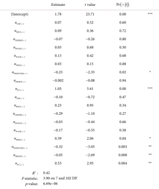
Table 5 reports the estimates of Equation (10) with M2 at time t−1 as the

regressor. Again, I find the last four types of shocks from the CEE model are correlated with the first lag of M2 on the R.H.S. of the CEE model.

Table 5. Estimation of the regression of the first lag of M2 on the lags of all innovations.

Estimate t value Pr

( )

(Intercept) 1.78 23.71 0.00 ***

GDP,t1

u − 0.07 0.52 0.60

RPCE,t1

u − 0.09 0.36 0.72

GDPDEF,t1

u − −0.07 −0.26 0.80

INVEST ,t1

u − 0.05 0.68 0.50

WAGE,t1

u − 0.13 0.42 0.68

PROD,t1

u − 0.03 0.15 0.88

FEDFUNDS,t1

u − −0.25 −2.35 0.02 *

PROFIT,t1

u − −0.002 −0.08 0.94

2, 1

M t

u − 1.03 5.61 0.00 ***

GDP,t2

u − −0.10 −0.72 0.47

RPCE ,t2

u − 0.23 0.95 0.34

GDPDEF,t2

u − −0.29 −1.10 0.27

INVEST ,t2

u − −0.03 −0.44 0.66

WAGE ,t2

u − −0.17 −0.55 0.58

PROD,t2

u − 0.39 2.06 0.04 *

FEDFUNDS,t2

u − −0.32 −3.05 0.003 **

PROFIT,t2

u − −0.05 −2.69 0.008 **

2, 2

M t

u − 0.53 2.95 0.004 **

2 R :

F-statistic: p-value:

0.42

3.90 on 7 and 102 DF 6.69e−06

error term is more likely to be correlated with the dependent variables and ex-planatory variables at the same time in the VAR model. Therefore, the impulse response results may be inferred from the biased coefficients of the SVAR model and we should be cautious to interpret these results.

4. Conclusions

462

different types of shocks may affect the variables in the structural VAR model over different horizons.

The academic significance of this paper is that my analysis sheds light on the potential problems of the impulse response functions and enhances our under-standing on how should we use the VAR model. The distortions of coefficients can be substantial in practice, which invalidates the traditional causal interpreta-tion of the responses of variables to a unit shock and overturns the standard view of how variables affect each other. When talks about the ceteris paribus, if outside variables will not change, the estimated coefficients of variables are ac-tually overestimated. The impulse response results and other conclusions in-ferred from the biased coefficients of the traditional SVAR models are no means settled issues and needed to be further studied.

The social significance of this paper is that the evidence from the SVAR models may be employed by many center banks to analyze the volatility trans-mission from a shock to the fluctuations in variables. For example, the oil price may not be the deep factor of recessions according to the instability of its esti-mated coefficient. It may be just the last straw that breaks the camel. Hence, oil price decreases may help the economy in the short horizon but the real problems which cause recessions still need to be solved.

The limitation of this research is that I only provide the possibility that the es-timations of the SVAR model may be biased, but this paper cannot explain how much it will affect the results of the existing literature. For some SVAR models, the biased coefficients may not be important at all because these parsimonious models may capture the main variables which can affect all other variables in the economy. These concerns are beyond the scope of this paper and need to be further studied.

Acknowledgements

I thank the Editor and the referee for their comments.

References

[1] Sims, C.A. (1980) Macroeconomics and Reality. Econometrica, 48, 1-48.

https://doi.org/10.2307/1912017

[2] Bernanke, B.S., Gertler, M. and Watson, M. (1997) Systematic Monetary Policy and the Effects of Oil Price Shocks. Brookings Papers on Economic Activity, 1997, 91- 157. https://doi.org/10.2307/2534702

[3] Hamilton, J.D. and Herrera, A. (2004) Oil Shocks and Aggregate Macroeconomic Behavior: The Role of Monetary Policy. Journal of Money, Credit, and Banking, 36, 265-286. https://doi.org/10.1353/mcb.2004.0012

[4] Hamilton, J.D. (1983) Oil and the Macroeconomy Since World War II. The Journal of Political Economy, 91, 228-248. https://doi.org/10.1086/261140

[5] Hooker, M.A. (1996) What Happened to the Oil Price-Macroeconomy Relation-ship? Journal of Monetary Economics, 38, 195-213.

[7] Blanchard, O.J. and Quah, D. (1988) The Dynamic Effects of Aggregate Demand and Supply Disturbances. National Bureau of Economic Research, Working Paper No. 2737, National Bureau of Economic Research, Cambridge, MA.

https://doi.org/10.3386/w2737

[8] Lv, Y. (2017) Selection of Macroeconomic Forecasting Models: One Size Fits All?

Theoretical Economics Letters, forthcoming.

[9] Lv, Y. (2017) How Can the Error Term Be Correlated with the Explanatory Va-riables on the R.H.S. of a Model? Theoretical Economics Letters, 7.

[10] Christiano, L.J., Eichenbaum, M. and Evans, C.L. (2005) Nominal Rigidities and the Dynamic Effects of a Shock to Monetary Policy. Journal of Political Economy, 113, 1-45. https://doi.org/10.1086/426038

Submit or recommend next manuscript to SCIRP and we will provide best service for you:

Accepting pre-submission inquiries through Email, Facebook, LinkedIn, Twitter, etc. A wide selection of journals (inclusive of 9 subjects, more than 200 journals)

Providing 24-hour high-quality service User-friendly online submission system Fair and swift peer-review system

Efficient typesetting and proofreading procedure

Display of the result of downloads and visits, as well as the number of cited articles Maximum dissemination of your research work

Submit your manuscript at: http://papersubmission.scirp.org/