Degradation Based Maintenance Using Stochastic Filtering for Systems under Imperfect Maintenance

Degradation-Based Maintenance Using Stochastic

Filtering for Systems under Imperfect Maintenance

ABSTRACT

The stationary Wiener process is widely used in modeling degradation processes, mainly due to the existence of an analytical expression of the first hitting time distribution. How-ever, it is only appropriate for modelling linearly drifted stochastic processes. This paper investigates a maintenance policy in which a family of non-stationary Wiener processes is used to simulate degradation phenomena. An approximation to the first hitting time distribution is invoked. A novel technique to treat imperfect maintenance is initiated by extending the improvement-factor method to the degradation rate function. A recursive filter is utilized to dynamically update the estimate of the degradation rate function. An algorithm, using the Laplace approximation, is developed for estimating model parame-ters. The applications of the proposed methods are demonstrated via both real-world and numerical examples.

Keywords: Maintenance; Degradation rate; Kalman filter; Laplace approximation; Non-stationary Wiener process.

1

INTRODUCTION

real-life practice (Bian and Gebraeel, 2012; Son et al., 2013; Zhou et al., 2011). The model in which the degradation rate increases with the level of degradation is, for example, used in modeling the growth of fatigue crack. Hudak et al. (1978) collected fatigue crack-size data from alloy to obtain information on crack-growth rates. See also Meeker and Escobar (1998) for modeling the size of fatigue crack as a function of the number of cycles. The convex curves in Figure 13.1 (Meeker and Escobar, 1998) verify that the crack-growth rate increases with the size of crack. Compared with linearly drifted degradation processes, a rather limited amount of research has been done on simulating non-linearly drifted degradation processes. The present paper investigates a maintenance policy in which a family of non-stationary Wiener processes is utilized to characterize degradation phenomena. A non-stationary Wiener process with drift functionv(t)and infinitesimal varianceσ2is defined byXt =v(t) +σWt. v(t)is a continuous, non-linear, real-valued function oft ≥0 withv(0) =0. The process{X_t, t≥0}has indepen-dent, non-stationary, and normally distributed random increments: For all 0≤s<t,X_t−X_s is independent ofXsand has the normal distributionN(v(t)−v(s), σ2(t−s)). The non-stationary Wiener process reduces to a stationary Wiener process withv(t)being a linear function oft.

A non-trivial problem in the degradation-based maintenance need be solved: the treatment to imperfect maintenance. Widely used assumptions on maintenance actions are good-as-new (or, perfect) and bad-as-old (or, minimal). It is more realistic in true experience that main-tenance actions merely restore a product’s condition to somewhere between good-as-new and bad-as-old. This type of maintenance is known as the imperfect maintenance. Extensive re-search on imperfect maintenance has been documented (Lindqvist, 2006; Nicolai et al., 2009; Zhang et al., 2013). One of the most popular treatments is the improvement-factor method. The improvement-factor method assumes that each maintenance action changes the time of the failure rate curve to some newer time but not all the way to zero; see Pham and Wang (1996). A general framework of the improvement-factor method is given as follows. Leth(t) (t ≥0)

denote the hazard rate function of the target product. Given that a maintenance action is per-formed at timet₁(>0), right after the maintenance action the hazard rate function assumes a new expression:βh(t−t1+αt1). Here,t−t1represents the time elapsed from the maintenance

action. 0<α<1 is an age-reduction factor. β>1 is a hazard-rate-increase factor. A represen-tative sample of works on improvement-factor method includes Chen et al. (2013), Doyen and Gaudoin (2011), Kurt and Kharoufeh (2010) and Li et al. (2012). However, the issue of treating imperfect maintenance in the context of degradation-based maintenance has not received much attention and remains widely open. By assuming that the degradation conforms to the non-stationary Wiener process,{X_t, t≥0}, the expected degradation up to timet isE[Xt] =v(t). Therefore, the first-order derivative ofv(t), denoted to bev0(t), can be treated as the degrada-tion rate funcdegrada-tion of the underlying degradadegrada-tion process. The degradadegrada-tion rate defined herein is the rate of accumulation of degradation. The degradation rate has been addressed a lot (Meeker and Escobar, 1998), and recent research can be found in Nikulin et al. (2010) and Rafiee et al. (2013). The improvement-factor method can be extended to the degradation rate function, i.e.

unchanged.

Another distinguishing feature of the proposed maintenance strategy is the utilization of stochastic filtering and the Laplace approximation. The bulk of the documented research on the improvement-factor method assumes a constant age-reduction factor and a constant hazard-rate-increase factor during a product’s whole operational life cycle. Apparently, the assumption of constant improving factors will be inappropriate and problematical in many circumstances. Since the operational condition varies wildly, each maintenance action should have a different degree of impact on the degradation rate. Therefore, the improving factors are indeed random variables, and the sequential maintenance actions result in a dynamical system. In the present paper, it is assumed that the improving factors are random variables following certain probabil-ity distributions. The realizations of the improving factors are estimated dynamically, by using stochastic filtering. Stochastic filtering is commonly used in the field of analyzing condition-monitoring data; see Ece and Basaran (2011), Lall et al. (2012) and Wang and Wang (2012). By assuming probability distributions for the improving factors, more unknown model param-eters will be introduced. The problem of estimating model paramparam-eters need be solved. When a likelihood function involves a multiple integral, the parameter-estimation problem will be very difficult. Most of the documented research on proposing maintenance policies made tangen-tial remarks on the parameter-estimation problem. The present paper uses Laplace’s method (Pinheiro and Bates, 1995) to deal with the multiple integral in a likelihood function.

In what follows, we first propose a degradation-based maintenance policy in which main-tenance actions are assumed to be imperfect. Then we dynamically estimate each realization of an improving factor by using a recursive filter. In the third step, we develop a procedure for estimating unknown model parameters. The remainder of the paper is organized as fol-lows. Section 2 is devoted to giving the framework of the advanced techniques. The method of treating imperfect maintenance via the degradation rate function is mathematically detailed. The proposed maintenance scheme is presented and the expression of the cost rate function is derived. Section 3 develops a stochastic filter for on-line estimating the realizations of an improving factor. Section 4 develops an algorithm for estimating unknown model parame-ters. Section 5 gives numerical examples to illustrate the applicability and competence of the advanced techniques. Section 6 outlines concluding remarks and future extensions.

2

MODEL FORMULATION

in which c=v(t)−bv(t), indicates that the degradation level remains unchanged. The case, in whichc6=v(t)−bv(t), indicates that the maintenance action results in a shift in the degra-dation level. Since the operational condition varies wildly, each maintenance action should have a different degree of impact on the degradation process. Therefore, in what follows, we assume that the factors,bandc, are random variables. Withb=1, we arrive at the bad-as-old assumption. Note that the proposed method involves the degradation-rate-reduction factor and the shifting factor, yet not the age-reduction factor. The topic of involving the age-reduction factor is beyond the scope of this paper. In terms of degradation-based maintenance, treating imperfect maintenance via the degradation rate function instead of the hazard rate function has two main advantages. Firstly, deriving the hazard rate function via the first hitting time distribution function is mathematically intractable, especially when the degradation process is non-stationary. Secondly, unlike the hazard rate which is unobservable and unmeasurable, the impact of maintenance actions on the degradation rate can be exteriorized from consecutive degradation measurements.

It is noteworthy that each realization of the shifting factor can be valued till the end, when all the other unknown parameters are estimated. For example, suppose that a main-tenance action is performed at time t1> 0. From time t1 forward, the degradation process

{X_t, t ≥0} is defined by X_t =b₁v(t+t₁) +c₁+σwt1+σWt. b1 and c1 are respective re-alizations of b and c at time t₁. w_t1 is a realization of W_t1. The degradation level right before the maintenance is x_t−

1 = v(t1) +σwt1. The degradation level right after the main-tenance is x_t+

1 = b1v(t1) +c1+σwt1. Suppose that another maintenance action is taken at timet₂>t₁. The degradation level at timet₂, right before the second maintenance, isx_t−

2 =

b₁v(t2+t1) +c1+σwt1+σwt2. wt2 is a realization ofWt2. Because the drift function remains unchanged between two consecutive maintenance actions, c1is eliminated in the degradation

increment: x_t− 2 −xt

+

1 =b1v(t2+t1) +σwt2−b1v(t1). Given data{xt − 1 , xt

+

1, xt −

2}, we first esti-mate the other model parameters based on the degradation incrementsx_t−

1 andxt − 2 −xt

+

1. Then, the realization of the shifting factor, c1, can be easily calculated based on the shift, x_t+

1 −xt − 1, and the estimated model parameters. Evidently, what plays a decisive role in estimating the other model parameters are the degradation increments. The shift of the degradation level is of no effect on the estimation of the other model parameters. Consequently, when estimating the other model parameters, there is no loss of generality by assuming that maintenance actions do not shift the degradation level. This assumption is made only for ease of exposition: without introducing too many subscripts or superscripts.

at the next DM point, and the process repeats. If t∗≤_M, the maintained system will be pre-ventively replaced at point i _M+t∗, and the process resumes. The DM points need not be equally spaced. Generalization of the proposed maintenance strategy to irregular DM points is a straightforward matter. The DM points could be included as decision variables driving the overall degradation-based maintenance policy. However, the complexity of inspections in practice might allow measurements to be taken only at selected epochs.

Figure 1 demonstrates a possible course of a replacement cycle, i.e. the time from the

in-installation inspection inspection and PM inspection potential inspection

Figure 1: A possible course of a replacement cycle.

stallation of a system to its replacement. At the first DM point,_M, after obtaining a degradation measurement and updating the degradation rate function, the optimal maintenance decision is to subject the system to the next inspection with no PM action taken at timeM. At the second DM point, 2_M, after obtaining another degradation measurement and updating the degradation rate function, the optimal maintenance decision is to subject the system to the next inspection with a PM action taken at time 2M. At the third DM point, the optimal maintenance decision is to preventively replace the system at time 3_M+t∗ with no PM action taken at time 3_M. If the system fails unexpectedly, it will be immediately replaced by a new physically and statistically identical one.

Unexpected failures can be observed instantaneously, each costingC_f. The average costs of a PM action and a preventive replacement areC_p andC_r, respectively. The cost of each inspection isCI. Practical conditions define the constraints of the maintenance costs as follows:

C_I <C_p<C_r<C_f.

Define a random variable,T_l, to be the first hitting time of the degradation process{X_t, t≥ 0}to a pre-determined threshold, l. Given that the maintained system is still operating at the

ith DM point,i_M, we introduce the following notation.

• X¨_i: history of degradation measurements up to and including theith, ¨X_i={x₁,x₂, ...,x_i}.

• _M¨_{i: history of PM actions up to and including the ith, ¨Mi ={m1 m2, ...,mi}. mi =0} indicates that no maintenance action is taken at theith DM point. m_i=1 indicates that an imperfect PM action is taken at theith DM point.

• ECi_pm(t): expected cost per unit time with a PM action taken at theith DM point, given that the system will be preventively replaced at timei_M+t.

• P_rul t|_X¨_{i, M}¨_i

=P T_l ≤t+i_M|_X¨_{i, M}¨_i

: remaining useful life distribution function at theith DM point (after the PM, if any).

The optimization is based on the minimization of a cost rate function. If the system is replaced, a new cycle of operation starts. The failure process constructs a renewal process. According to the renewal theorem, the long-run cost rate is equal to the expected cost in one renewal cycle divided by the expected length of the renewal cycle. Suppose that a PM action is taken at time

i_M(instantaneously after theith inspection) and that a preventive replacement is scheduled to be performed at timei_M+t. We have

ECi_pm(t) = icI+∑

i

j=1mjcp+cr

1−P_rul t|X¨_i, M¨_i−1,m_i=1+ (cf+cr)Prul t|X¨i, M¨i−1,mi=1

i_M+t

1−P_rul t|_X¨_{i, M}¨_i−1,mi=1

+Rt

0s dPrul s|X¨i, M¨i−1,mi=1

= icI+∑

i

j=1mjcp+cr+cfPrul t|X¨i, M¨i−1,mi=1

i_M+t−Rt

0Prul s|X¨i, M¨i−1,mi=1

ds .

Here,ic_I is the overall inspection cost.∑i_j=1mjcpis the overall PM cost.cr

1−P_rul t|X¨_i, M¨_i

is the expected cost of a preventive replacement at time i_M+t. (cf+cr)Prul t|X¨i, M¨i

is the expected cost of an unexpected failure within interval (i_M, i_M+t). The denominator is the expected length of a replacement cycle:

E[Tl] = iM+E[Tl−iM|Tl>iM] =iM+ Z ∞

0

s dP_rul s|X¨_i, M¨_i−1,m_i=1

= i_M+t1−P_rul t|X¨_i, M¨_i−1,m_i=1+

Z t

0

s dP_rul s|X¨_i, M¨_i−1,m_i=1.

Given no maintenance action at timei_Mand a scheduled preventive replacement at timei_M+t, we have

EC_nai (t) = icI+∑

i

j=1mjcp+cr

1−P_rul t|_X¨_{i, M}¨_i−1,mi=0

+ (c_f+c_r)P_rul t|_X¨_{i, M}¨_i−1,mi=0

i_M+t1−P_rul t|X¨_i, M¨_i−1,m_i=0+Rt

0s dPrul s|X¨i, M¨i−1,mi=0

= icI+∑

i

j=1mjcp+cr+cfPrul t|X¨i, M¨i−1,mi=0

i_M+t−Rt

0Prul s|X¨i, M¨i−1,mi=0

ds .

Denotet_p∗to be the optimal preventive-replacement time that minimizes the cost rate function

ECi_pm(t). Denotet_n∗to be the optimal preventive-replacement time that minimizes the cost rate functionEC_nai (t).

• IfECi_pm(t∗_p)<EC_nai (t_n∗), a maintenance action is taken at timei_M, and the system will be preventively replaced at timei_M+t∗_p i f t∗_p<_Mor will be inspected at the next DM point(i+1)_M i f t∗_p>_M.

• IfECi_pm(t∗_p)>EC_nai (t_n∗), no maintenance action is taken at timei_M, and the system will be preventively replaced at timei_M+t_n∗ (i f t_n∗<_M)or will be inspected at the next DM point(i+1)_M(i f t_n∗>_M).

(Buonocore et al., 2011). For a non-linearly drifted stochastic process, deriving the remaining useful life distribution function involves solving the Fokker-Planck-Kolmogorov equation with boundary constraints (Cox and Miller, 1965). Many works, such as Gebraeel et al. (2005), Park and Padgett (2005) and Wang (2010), make non-linear transformations on degradation data and fit the stationary Wiener process to the transformed data. An implicit assumption in the data-transformation approach is that the random part of the transformed process is still Brownian motion, which may not always be the case (Si et al., 2012). To reduce the heavy computational burden, we develop, in Section 3, a closed-form expression approximating the remaining useful life distribution function.

3

ON-LINE UPDATING

A commonly used formulation of the drift function in the non-stationary Wiener process is given byv(t) =λtθ (Son et al., 2013; Wang et al., 2014). λ >0 is a scale parameter. θ >0 is a shape parameter. The degradation rate function is the derivative of the drift function: v0(t) =

λ θtθ−1. If a maintenance action is performed at timeM, immediately after the maintenance the degradation rate function assumes a new expression: b₁v0(t) =b₁λ θtθ−1, t >M. b1 is a

realization of b. We might defineλ1 =b1λ and write b1v

0

(t) =λ1θtθ−1. Instead of saying

that the degradation rate function changes from v0(t)to b₁v0(t), it is equivalent to saying that immediately after the maintenance the scale parameter changes from λ to λ1. Therefore, to

update the estimate of the degradation rate function, it is sufficient to update the estimate of the scale parameter. An updating procedure, i.e. the Kalman filter, is developed herein for recursively producing a statistically optimal estimate of the scale parameter. The Kalman filter (Chui and Chen, 2009) is an algorithm which iteratively involves two steps: the predict step and the update step. In the predict step, the Kalman filter produces an estimate of the state and an estimate of the covariance matrix. The estimate of the state is termed as the a prior state estimate. The estimate of the covariance matrix is termed as the a prior estimate error covariance. In the update step, the Kalman filter produces the a posterior state estimate and the a posterior estimate error covariance by using a weighted average. Theory, methods and applications of the Kalman filter have been extensively reported in operational research, such as Carr and Wang (2011), Humpherys et al. (2012), and Kluge et al. (2010); see Si et al. (2011) for a recent review.

Denote λi (i=1,2,3, ...) to be the hidden true value of the scale parameter at time iM before any maintenance action. Denotex_i (i=0,1,2, ...) to be the degradation measurement obtained at timei_Mwithx₀=0. Denotey_i(i=1,2,3, ...) to be theith degradation increment:

yi=xi−xi−1. Fori=1,2,3, ..., we have the process equation

λi=µi−1λi−1+δi−1,

and the measurement equation

y_i=ρiλi+ωi.

The derivation of the process equation and the measurement equation is given in the Appendix. The process noise is additive, white and normally distributed with zero mean and variance

Denote ˆλ_i− to be the a prior estimate ofλi, calculated by utilizing the knowledge of ¨Xi−1

and ¨M_i−1. Denote ˆλito be the a posterior estimate ofλi, calculated by utilizing the degradation increment, y_i, and the a prior estimate, ˆλ_i−. When making the a posterior estimate, ˆλi, be a linear combination of the a prior estimate, ˆλ_i−, and the degradation increment,yi, we arrive at the Kalman filter which is a minimum mean-square error estimator. DefineP_i−to be the a prior estimate error variance:

P_i− =E[(λi−λˆi−)(λi−λˆi−)].

DefineP_ito be the a posterior estimate error variance:

Pi=E[(λi−λˆi)(λi−λˆi)].

Fori=1, 2, 3, ..., the recursive estimation of the scale parameter entails the following updating equations (Welch and Bishop, 2006):

• state estimate propagation

ˆ

λ_i− =µi−1λˆi−1,

• estimate error variance propagation

P_i−=µ_i−2 ₁Pi−1+Qi−1,

• Kalman gain

G_i= P

− i ρi

P_i−ρ_i2+σ2M,

• state estimate update

ˆ

λi=λˆ_i−+Gi(yi−ρiλˆ_i−),

• estimate error variance update

P_i= (1−G_iρi)P_i−.

The starting values, ˆλ0andP0, are chosen arbitrarily, reflecting our best assessment of the scale

parameter prior to any DM information. Substituting ˆλ_i− andGiinto the state-estimate-update equation, we have

ˆ

λi=µi−1λˆi−1+

(µ_i−2₁Pi−1+Qi−1)ρi

(µ_i−2 ₁Pi−1+Qi−1)ρ_i2+σ2M

×y_i−ρiµi−1λˆi−1

.

SubstitutingP_i− andG_iinto the estimate-error-variance-update equation, we have

P_i= (µ 2

i−1Pi−1+Qi−1)×σ2M (µ_i−2 ₁Pi−1+Qi−1)ρ_i2+σ2M

.

the analytical form of the density function, P(T_l=t), cannot be constructed. Si et al. (2012) developed a closed-form expression1approximating the density function, which is given by

˜

f(t; λ, θ, σ, l) =κ×l+ (θ−1)λt θ

σ √

2πt3 exp −

l−λtθ2

2σ2_t

!

, t≥0. (1)

Here,κ is a normalizing constant:

1

κ =

Z

0

l+ (θ−1)λtθ

σ √

2πt3 exp −

l−λtθ2 2σ2_t

!

dt.

Given that the maintained system is still operating at timei_M (i=1,2,3, ...), once the degra-dation measurementx_i(<l) is obtained, we immediately update the estimate of the scale pa-rameter to be ˆλi. If there is no maintenance action at timeiM, the value of the scale parameter remains unchanged and is estimated by ˆλi. From timeiMforward, the degradation process is defined by

X_s+iM−XiM=λˆi(s+iM)θ−λˆi(iM)θ+σWs, s≥0.

We might denoteXs+iM−XiMbyYsi:Ysi=Xs+iM−XiM. The remaining useful life of the system

at timei_Mis indeed the first hitting time of the degradation process{Y_si, s≥0}to the threshold

l_i=l−x_i. The degradation process{Y_si, s≥0} is a non-stationary Wiener process with drift function

υi(s) =λˆi(s+iM)θ−λˆi(iM)θ.

We haveυi(0) =0. Therefore, according to Equation (1), the remaining useful life distribution function,P_rul t|X¨_i, M¨_i−1, m_i=0, can be approximated by

˜

fi(t) =

Z

0

κi×li−υi(s) +θ ˆ

λis(s+iM)θ−1

σ √

2πs3 exp −

[li−υi(s)]2 2σ2_s

!

ds, t ≥0, (2)

withκibeing the normalizing constant

1

κi =

Z

0

l_i−υi(s) +θλˆis(s+iM)θ−1

σ √

2πs3 exp −

[li−υi(s)]2 2σ2s

!

ds. (3)

If a maintenance action is performed at timei_M, then after the maintenance the scale parameter is estimated by ˆλ_i−₊₁=µλˆi. The remaining useful life distribution function,Prul t|X¨i, M¨i−1, mi=1

, can be approximated by ˜fi(s) in which ˆλi is replaced by ˆλ_i−₊₁. By using the closed-form ex-pression, ˜f_i(s), approximating the remaining useful life distribution function, P_rul t|X¨_i, M¨_i, the expected cost rate functions,ECi_pm(t)andEC_nai (t), can be readily minimized.

4

PARAMETER ESTIMATION

In the proposed maintenance policy we have five model parameters: three degradation pa-rameters, {λ, θ, σ}, and two maintenance parameters, {µ, Q}. When estimating the scale parameter by the Kalman filter, the other model parameters, θ, σ, µ andQ, are assumed to be known. It is worth stressing that the performance of the recursive filter relies on whether or not the other four parameters are accurately estimated. We develop herein an approxi-mating approach to estiapproxi-mating the model parameters: θ, σ, µ and Q. Up to time t, with

n_M≤t <(n+1) _M, we obtain degradation measurements ¨X_n ={x₁,x₂, ...,x_n} and mainte-nance indicators ¨M_n−1={m₁,m₂, ...,m_n−1}. Since the(n+1)th degradation measurement is not available, thenth maintenance indicator, mn, is of no help in estimating the model param-eters and hence omitted. Note that if a maintenance action is performed, the realization of the degradation-rate-reduction factor, on which the likelihood function is conditioned, is latent. Define a column vectorbbbn−1= (b1,b2, ...,bn−1)T in whichbi (1≤i≤n−1) is theith real-ization of b. By the superscript T, we mean the transpose of a vector/matrix. If there is no maintenance at timei_M, we simply set b_i=1. For illustrative purpose, we might assume that

mi=1 for all 1≤i≤n−1. Generalization to mi=0, for some 1≤i≤n−1, is straightfor-ward. Given degradation measurements ¨X_n, a general formulation of the likelihood function of the parametersΘ={λ, θ, σ, µ, Q}is given by

` Θ|X¨n

=

Z +∞

−∞

· · · Z +∞

−∞

1

(σ √

2π_M)nexp

 −

(x₁−λ ρ1)2

2σ2_M −

1 2σ2_M

n

∑

i=2

x_i−x_i−1− i−1

∏

j=1 b_jλ ρi

!2 

× 1

(√2πQ)n−1exp −

n−1

∑

j=1

(bj−µ)2 2Q

!

dbbb_n−1.

Each evaluation of` Θ|X¨n

will, in general, require numerical approximation of the integral of dimension n−1. When the number of maintenance actions is large, maximizing ` Θ|X¨n

is extremely difficult and time-consuming. One possible solution to overcoming the compu-tational inefficiency is to use approximations to the likelihood function. We use the Laplace approximation to serve the purpose. Once the estimates of the model parameters are obtained, the realizations of the shifting factor will be readily determined based on the estimates and the degradation measurements.

Define a new functiongr Θ, bbbn−1, X¨n

:

gr Θ,bbbn−1, X¨n

= (x1−λ ρ1) 2

2σ2M + 1 2σ2M

n

∑

i=2

x_i−x_i−1− i−1

∏

j=1 b_jλ ρi

!2

+

n−1

∑

j=1

(bj−µ)2 2Q .

The likelihood function,` Θ|X¨n, can be re-formulated to be

` Θ|X¨n

= (2π σ2_M)−n/2

Z +∞

−∞

· · · Z +∞

−∞

(2πQ)−(n−1)/2exp −gr Θ, bbbn−1, X¨n

dbbb_n−1.

Letgr0(Θ,bbbn−1, X¨n)denote the first order partial derivative ofgr(Θ,bbbn−1, X¨n)with respect to

bbb_n−1:

gr0(Θ, bbbn−1, X¨n) =

∂gr(Θ, bbbn−1, X¨n)

Letgr00(Θ,bbbn−1, X¨n)denote the second order partial derivative ofgr(Θ,bbbn−1, X¨n)with respect tobbbn−1:

gr00(Θ, bbbn−1, X¨n) =

∂2gr(Θ, bbbn−1, X¨n)

∂bbbn−1∂bbbT_n−1 .

The expressions ofgr0(Θ,bbbn−1, X¨n)andgr 00

(Θ, bbbn−1, X¨n)are given in the Appendix. Let ˆbbbn−1

denote the minimizer ofgr(Θ, bbbn−1, X¨n):

ˆ

b b

b_n−1=arg min bbb

gr(Θ, bbb, X¨n).

Becausegr(Θ, bbbn−1, X¨n) is differentiable, we havegr 0

(Θ, bbbˆn−1, X¨n) =0. The calculation of ˆ

bbb_n−1 is straightforward, for which standard and efficient code is available. The second order Taylor expansion ofgr Θ, bbbn−1, X¨n

around ˆbbb_n−1is:

gr Θ, bbbn−1, X¨n

≈grΘ, bbbˆn−1, X¨n

+1

2[bbbn−1− ˆ

b

bb_n−1]Tgr00(Θ, bbbˆn−1, X¨n)[bbbn−1−bbbˆn−1],

in which the linear term of the Taylor series vanishes since gr0(Θ, bbbˆn−1, X¨n) =0. Treating

[gr00(Θ,bbbˆn−1, X¨n)]−1as a covariance matrix, we have

q

|[gr00(Θ,bbbˆn−1, X¨n)]−1|=

Z +∞

−∞

· · · Z +∞

−∞

1

√

(2π)n−1exp

−1

2[bbbn−1−bbbˆn−1]

T_gr00₍

Θ,bbbˆn−1, X¨n)[bbbn−1−bbbˆn−1]

dbbb_n−1,

in which |[gr00(Θ, bbbˆn−1, X¨n)]−1|is the determinant of[gr 00

(Θ, bbbˆn−1, X¨n)]−1. Substituting the second order Taylor expansion into the likelihood function,` Θ|X¨n

, we have

` Θ|X¨n≈

1

p

(2π σ2_M)nexp

−gr

Θ, bbbˆn−1, X¨n

1 p

Qn−1

q

|[gr00(Θ, bbbˆn−1, X¨n)]−1|.

The Laplace approximation to the log-likelihood function is

`LA

Θ|X¨n, bbbˆn−1

∼

=−nlog(σ)−gr

Θ, bbbˆn−1, X¨n

−n−1

2 log(Q) + 1

2log(|[gr 00

(Θ,bbbˆn−1, X¨n)]−1|).

Let ˆΘk ={λˆk, θˆk, σˆk, µˆk, Qˆk} denote the estimates of the model parameters, obtained after thekth iteration (k=1, 2, ...). Given the current estimates, ˆΘk, the LA algorithm in the

(k+1)th iteration evolves as follows.

Step-One: Minimize gr(Θˆk, bbbn−1, X¨n) with respect to bbbn−1 and substitute the minimizer

ˆ

b

bb(_n−k+₁1) into the Laplace approximation:`LA

Θ|X¨n, bbbˆ

(k+1)

n−1

.

Step-Two: Maximize the Laplace approximation `LA

Θ|X¨n, bbbˆ

(k+1)

n−1

with respect to Θ and

update ˆΘk by the maximizer ˆΘ(k+1).

The LA algorithm alternates between the minimizing step and the maximizing step until certain convergence criterion is met. In comparison to directly maximizing` Θ|X¨n

5

NUMERICAL EXAMPLES

The following data-generating method is to generate degradation data from the non-stationary Wiener process. For later reference, we term it as the DG method. At timeM, we randomly generate an observation of the degradation, denoted byx1, from the normal distributionN(λ Mθ , σ2M).

• If a maintenance action is then performed at time M, the value of the scale parameter changes, immediately after the maintenance, from λ to b1λ. b1 is a realization of b,

which is randomly generated from the normal distribution N(µ,Q). At time 2M, we randomly generate a degradation increment, denoted byy2, from the normal distribution N b₁λ(2θ−1)Mθ, σ2M.

• If no maintenance action is performed at time_M, at time 2_M we randomly generate a degradation increment,y2, from the normal distributionN(λ(2θ−1)Mθ, σ2M).

The degradation measurement obtained at time 2_Mis denoted byx₂:x₂=x₁+y₂. By analogy, at timei_M(i=2,3,4, ...), we randomly generate a degradation incrementy_ifrom the normal distribution N(∏i−_j=1₁bm_jjλ[iθ−(i−1)θ]Mθ, σ2M). The ith degradation measurement is de-noted by x_i: x_i=x_i−1+y_i. {b_j, j=1,2,3, ...} are all randomly generated from the normal distributionN(µ,Q). {mj, j=1,2,3, ...}are the maintenance indicators defined in Section 2.

5.1

Simulation Study

Maintenance decisions are made based on the current estimate of the scale parameter. There-fore, before implementing the maintenance policy, we make an investigation into the per-formance of the proposed recursive filter. Simulated degradation data, generated by the DG method, are used to serve the purpose. The degradation parameters are assigned with values λ =7e-5,θ =2.5 andσ =2. The maintenance parameters are assigned with valuesµ =0.7 and Q=0.1. The length of the DM interval is 100 units of time, i.e. M=100. The mainte-nance indicators {m_j, j =1,2,3, ...} are randomly generated from the Bernoulli distribution with success probability 0.5. Hence, the probability of taking a maintenance action is 0.5. The starting values for the recursive filter are set to beλ0=1 andP0=1. In comparison to the true

value,λ =7e-5, the starting value,λ0, is assigned with a very big deviation. The prior estimate

error variance,P₀, is also assigned with a big value.

0 5 10 15 20 25 30 0

0.2 0.4 0.6 0.8 1 1.2 1.4 1.6

1.8x 10

−4

DM number i

λ

true value estimate

Figure 2: True values and estimates of the scale parameter.

0 10 20 30

−2 0 2 4 6 8 10

12x 10

−5

DM number i

deviation

0 10 20 30

0 0.5 1 1.5 2 2.5 3 3.5

4x 10

−8

DM number i

P i

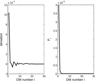
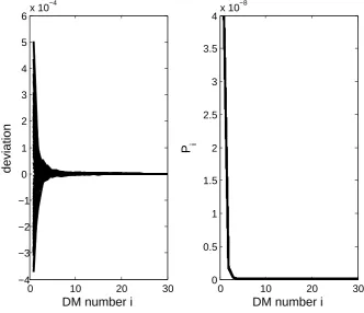
different degradation data sets. Run the recursive filter on the data sets respectively. The 100 evolving paths of the deviation{λiˆ −λi, i=1,2,3...}and 100 evolving paths of the estimate error variance {P_i, i=1,2,3...} are plotted in Figure 4. In Figure 4, all the deviation paths

0 10 20 30

−4 −3 −2 −1 0 1 2 3 4 5

6x 10

−4

DM number i

deviation

0 10 20 30

0 0.5 1 1.5 2 2.5 3 3.5

4x 10

−8

DM number i

P i

Figure 4: Evolving paths of{λˆi−λi, i=1,2,3...}and{Pi, i=1,2,3...}with 100 samples.

and variance paths converge rapidly to zero, showing the robustness of the stochastic filtering in assessing the scale parameter.

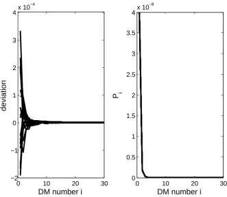
A sensitivity study is conducted to investigate the impact of the number of maintenance actions on the performance of the Kalman filter. Intuitively, with the maintenance actions being more intensive, the scale parameter should be more difficult to assess. With all the other parameters being the same, we gradually increase the success probability in the Bernoulli distribution from 0.05 to 0.95 with step size 0.05. For each value of success probability, use the DG method to generate a degradation data set and run the recursive filter on the simulated degradation data. The 19 evolving paths of the deviation{λiˆ −λi,i=1,2,3...}and 19 evolving paths of the estimate error variance{P_i, i=1,2,3...}are plotted in Figure 5. In Figure 5, both the deviation and the estimate error variance convergence rapidly to zero. In each of the 19 cases, the Kalman filter can return an accurate estimate of the scale parameter requiring only about 15 degradation measurements. Therefore, the performance of the proposed Kalman filter is insensitive to the frequency of maintenance.

0 10 20 30 −2

−1 0 1 2 3

4x 10

−4

DM number i

deviation

0 10 20 30

0 0.5 1 1.5 2 2.5 3 3.5

4x 10

−8

DM number i

P i

Figure 5: The impact of the number of maintenance actions on the performance of the Kalman filter.

realization of bmay be negative or larger than one, which is inconsistent with the fact. If a realization ofbis larger than one, then after the maintenance the system deteriorates faster. If a realization ofb is negative, then after the maintenance the degradation decreases over time. To make the realization constrained in the interval(0,1], the variance,Q, cannot be too large. Future work can be done to develop a suitable distribution forbwith domain(0,1]. The topic is beyond the scope of this paper. From the mathematical point of view, for illustrative purpose, we gradually increase the variance in the normal distribution from 0.01 to 1 with step size 0.01. The starting values for the filter areλ0=1 andP0=10. All the other parameters remain

the same. The 100 evolving paths of the deviation {λˆi−λi, i=1,2,3...} and 100 evolving paths of the estimate error variance {P_i, i=1,2,3...}are plotted in Figure 6. Figure 6 shows that the estimate converges rapidly to the true value even ifQandP0 are relatively large. The

convergent sequences, {λˆi−λi, i=1,2,3...} and{Pi, i=1,2,3...}, verify the robustness of the Kalman filter. Therefore, we say that the Kalman filter is insensitive to the starting values, the number of maintenance actions and the variance of the degradation-rate-reduction factor. As long as the four parameters,θ,σ,µ andQ, are accurately assessed, the Kalman filter is able to produce an accurate estimate on the scale parameter with small number of observations.

5.2

Real Data Analysis

measure-0 10 20 30 −6

−4 −2 0 2 4

6x 10

−4

DM number i

deviation

0 10 20 30

0 0.5 1 1.5 2 2.5 3 3.5

4x 10

−8

DM number i

P i

Figure 6: The impact of the varianceQon the performance of the Kalman filter.

ments (along the sense axis). The experimental degradation data from 5 monitored gyros are shown in Table 1. In the experiment, the drift degradation of each gyro was monitored every

Table 1: Drift degradation data from an inertial platform.

gyroscopic drift (◦/h)

time (h) item 1 item 2 item 3 item 4 item 5 2.5 0.0507 0.1300 0.0135 0.0928 0.1052 5.0 0.1789 0.2554 0.0309 0.2633 0.1996 7.5 0.2059 0.3153 0.0077 0.3010 0.2927 10.0 0.2548 0.3966 0.1510 0.3515 0.3060 12.5 0.3117 0.2424 0.1162 0.2818 0.2860 15.0 0.5236 0.3473 0.0237 0.4375 0.2918 17.5 0.61140.61140.6114 0.4994 0.2681 0.3357 0.3540 20.0 0.66160.66160.6616 0.71050.71050.7105 0.4934 0.4413 0.4326 22.5 1.81661.81661.8166 2.63992.63992.6399 0.65130.65130.6513 0.81570.81570.8157 0.5042

0 5 10 15 20 25 0

0.5 1 1.5 2 2.5 3

CM epoch (hours)

gyroscopic drift (

° /hour)

Figure 7: Drift degradation paths of gyros.

obtained as ˆλ =1.3082e-18, ˆθ =13.2024 and ˆσ =0.1604. The maximized log-likelihood is -2.1184. If the drift function takes the exponential form: v(t) =λexp(θt). The corresponding maximum likelihood estimates of the degradation parameters are ˆλ =1.5592e-6, ˆθ =0.5920 and ˆσ =0.1602. The maximized log-likelihood is -2.0684. Hence, in terms of the fitness, the power model,v(t) =λtθ, is practically equal to the exponential model,v(t) =λexp(θt).

We then implement the proposed maintenance policy on the inertial platforms to illustrate the procedure for determining the optimal maintenance actions. At each DM point, having obtained the drift degradation measurement, engineers have to decide whether or not to pre-ventively maintain the target inertial platform. Preventive maintenance on the inertial platform is assumed to be imperfect, e.g., replacing one of the gyros. Unexpected failure of the inertial platform is hazardous and costly. The inertial platform itself is also very expensive. A high-end marine-grade inertial navigation system may cost over 1 million dollars. In the present paper we consider an industrial-grade inertial navigation system, and the cost configurations are specified as follows. The cost of replacing an inertial platform is c_r=$2000. The cost of an unexpected failure of the inertial platform isc_f =$10000. The cost of each inspection is

c_I =$20. A PM action on the inertial platform costsc_p=$100. Here,c_pneed not be constant during the whole replacement cycle, but can vary according to practical conditions.

Because there was no maintenance in the experiment, we use the DG method to simu-late degradation measurements. The degradation parameters assume the values estimated: λ =1.3082e-18, θ =13.2024 and σ =0.1604. To be consistent, the maintenance parame-ters assume the same values as what have been assigned in Section 5.1: µ =0.7 andQ=0.1. The starting value, λ0, is assigned with the estimate obtained based on the drift degradation

the drift degradation measurements of one individual gyro. Calculate the variance of the four estimates which are obtained based on the first four gyros, respectively. The starting value,P0,

is assigned with the variance of the four estimates: P₀=3.5995e-11. Once a new degradation measurement is obtained, we immediately update the a posterior estimate of the scale parame-ter and the a posparame-terior estimate error variance. Under the preceding parameparame-ter settings and cost configurations, one realization of the replacement cycle is described in Table 2.

Table 2: An optimal maintenance scheme implemented on the inertial platform.

i 1 2 3 4

ECi_pm(t∗_p) 3.7554e+03 2.2660e+03 0.2343e+03 1.0903e+03

EC_nai (t_n∗) 3.7879e+03 2.2745e+03 0.2288e+03 1.0973e+03

m_i 1 1 0 1

t∗_p 3.0116 3.0740 2.7820 2.6435

t_n∗ 4.0323 2.8474 2.5591 2.2610

λi 1.3082e-18 1.0685e-18 7.1367e-19 7.1367e-19 ˆ

λi 2.1445e-08 2.1887e-10 1.5639e-14 6.8281e-15

i 5 6 7 8

ECi_pm(t∗_p) 0.8842e+03 0.7564e+03 0.1309e+03 0.1274e+03

EC_nai (t_n∗) 0.8898e+03 0.7608e+03 0.1284e+03 0.1237e+03

m_i 1 1 0 0

t∗_p 3.2007 3.1802 3.6786 1.7637

t_n∗ 2.7598 2.6083 3.2651 1.5856 λi 5.2930e-19 2.9720e-19 1.3367e-19 1.3367e-19 ˆ

λi 4.3790e-16 7.0723e-17 2.1252e-18 7.7187e-19

According to Table 2, the decision-making process involves the following steps. At time M, since the minimized cost rateEC1_pm(t∗_p)is smaller than its counterpartEC_na1 (t_n∗), the system is preventively maintained at time t =_M. Since the optimal preventive-replacement time t∗_p

is larger than the DM interval, the drift degradation is monitored at the second DM point. Likewise, at the ensuing DM point 2M, the optimal maintenance decision is to measure the degradation at time 3_Mwith a maintenance action taken at time 2_M. At time 3_M, since the minimized cost rate EC3_pm(t∗_p) is larger than its counterpartEC_na3 (t_n∗), the system is left intact and the degradation is measured at time 4M. At time 8M, the optimal maintenance decision is to leave the system intact. Since the optimal preventive-replacement timet_n∗is smaller than the DM interval, the system is preventively replaced at timet =8_M+1.5856, if it survives to this point. Table 2 also lists the true value and estimate of the scale parameter at each DM point. Because the initial estimate error variance,P₀, is assigned with a large value, the first few estimates, e.g. {λˆ1, λˆ2, λˆ3, λˆ4}, have a large error. However, after obtaining 8 measurements,

the filter is able to return a good estimate.

5.3

Parameter Estimation

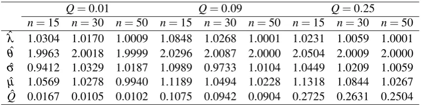
of time, i.e. _M=1. To show the robustness of the Laplace’s method, we vary the data size in {15, 30, 50}and the variance of the degradation-rate-reduction factor in {0.01, 009, 0.25}. The number 15 corresponds to a small sample; the number 30 corresponds to a moderate sam-ple; the number 50 corresponds to a large sample. The value 0.01 corresponds to a small variance; the value 0.09 corresponds to a moderate variance; the value 0.25 corresponds to a large variance. The approximating maximum likelihood estimates are tabulated in Table 3.

Table 3: Approximating maximum likelihood estimates of the model parameters.

Q=0.01 Q=0.09 Q=0.25

n=15 n=30 n=50 n=15 n=30 n=50 n=15 n=30 n=50 ˆ

λ 1.0304 1.0170 1.0009 1.0848 1.0268 1.0001 1.0231 1.0059 1.0001 ˆ

θ 1.9963 2.0018 1.9999 2.0296 2.0087 2.0000 2.0504 2.0009 2.0000 ˆ

σ 0.9412 1.0329 1.0187 1.0989 0.9733 1.0104 1.0449 1.0209 1.0059 ˆ

µ 1.0569 1.0278 0.9940 1.1189 1.0494 1.0228 1.1318 1.0844 1.0267 ˆ

Q 0.0167 0.0105 0.0102 0.1075 0.0942 0.0904 0.2725 0.2631 0.2504

Table 3 shows that the general likelihood function can be well approximated by the Laplace approximation. When the sample size is moderate or large, approximating maximum likelihood estimates concentrate near the true values even whenQis large. When the sample size is small, the LA algorithm can still return useful estimates. For a fixed sample size, the variance of the degradation-rate-reduction factor is of no impact on the performance of the LA algorithm. Note that a crucial step in the LA algorithm is the calculation of the minimizer

ˆ

b b

b_n−1=arg min bbb gr(Θ,

b b b, X¨_n).

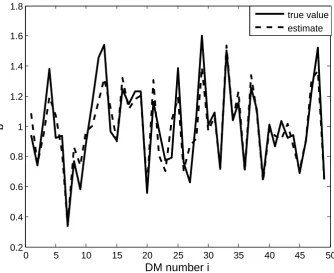
If ˆbbb_n−1is close tobbb_n−1, then the Laplace approximation is close to the general likelihood func-tion. To take a deeper look into the evolution of the LA algorithm, after obtaining a set of approximating maximum likelihood estimates ˆΘ={λˆ, θˆ, σˆ, µˆ, Qˆ}, we calculate the mini-mizer ofgr(Θˆ, bbb, X¨n). For Q=0.09 andn=50, Figure 8 plots the simulated 49 realizations of the degradation-rate-reduction factor, i.e. bbb_n−1, and the minimizer of gr(Θˆ, bbb, X¨n). The solid line threads the realizations, and the dashed line threads the estimates. Evidently, the minimizer ˆbbb_n−1 is close tobbb_n−1. Hence, Figure 8 explains to some extent the reason for the good performance of the LA algorithm.

6

CONCLUSIONS

0 5 10 15 20 25 30 35 40 45 50 0.2

0.4 0.6 0.8 1 1.2 1.4 1.6 1.8

DM number i

b

true value estimate

Figure 8: Simulated realizations of the degradation-rate-reduction factor and the corresponding estimates.

• As mentioned before, the extended improvement-factor method involves the degradation-rate-reduction factor and the shifting factor, yet not the age-reduction factor. Future work can be done to develop a model with three improving factors.

• The choice of a distribution for the degradation-rate-reduction factor,b, is of great im-portance. Therefore, it is of interest to develop a suitable distribution with domain(0,1]

forb. An alternative approach, when the variance ofbis small, is to assume that bis a constant.

• The non-stationary Wiener process represents a family of continuous yet non-monotone diffusion processes. Other stochastic processes, such as non-stationary Gamma processes and non-stationary inverse Gaussian processes, can be used to characterize monotonically drifted diffusion processes. Developing stochastic filters which are built on monotoni-cally drifted diffusion processes is an issue of great importance.

APPENDIX A

Derivation of the Process Equation and the

Measurement Equation

Note that the value of the scale parameter at time(i−1)_M(right after the maintenance, if any) is identical to the value of the scale parameter at timei_M(before any maintenance action). The degradation rate function over theith interval is

The drift function over theith interval is

vi(t)∼=λitθ, (i−1)M<t<iM.

The symbol∼=denotes equality up to an additive constant. With the assumption that the degra-dation conforms to the non-stationary Wiener process, we have

X_iM−X_(i−1)M = λi(iM)θ−λi[(i−1)M]θ+σWM

= ρiλi+σW_M,

with the constant being eliminated andρidefined by

ρi= (iM)θ−[(i−1)M]θ.

Hence, we have the measurement equation

y_i=ρiλi+ωi,

in whichωiis a realization ofσW_Mand is termed as the measurement noise.

With the operational condition varying wildly, each maintenance action should have a dif-ferent degree of impact on the degradation process. To characterize the uncertainty, we assume that the degradation-rate-reduction factor,b, is normally distributed with meanµ and variance

Q. µ andQare two unknown model parameters that will be estimated in Section 4. If no main-tenance action is taken at time(i−1)_M, we haveλi=λi−1. If a maintenance action is taken at

time(i−1)_M, thenλi=bi−1λi−1is normally distributed with meanµ λi−1and varianceQλ_i−2₁.

b_i−1is a realization ofb. The relationship betweenλi−1andλican be summarized into

λi=µi−1λi−1+δi−1.

If no maintenance action is taken at time(i−1)_M, thenµi−1=1 andδi−1=0. If a maintenance

action is taken at time(i−1)_M, then µi−1=µ andδi−1is normally distributed with mean 0

and variance Qλ_i−2₁. δi−1 is termed as the process noise. For ease of exposition, we might

sayδi−1 is normally distributed with mean 0 and varianceQi−1, in whichQi−1 is defined by Q_i−1 =Qλ_i−2₁mi−1. Note that, with bi−1 being independent of λi−1, Qi−1 is independent of Q_i−2. The degradation-rate-reduction factor need not be normally distributed. The topic of non-normal degradation-rate-reduction factor is beyond the topic of this paper.

APPENDIX B

Derivation of

gr

(

Θ

,

b

b

b

,

X

¨

)

The first order partial derivative ofgr(Θ, bbbn−1, X¨n)with respect tobk(1≤k≤n−1) is given by

∂gr(Θ, bbbn−1, X¨n)

∂b_k = 1

σ2M× n

∑

i=k+1

x_i−x_i−1− i−1

∏

j=1 b_jλ ρi

!

−1

b_k

i−1

∏

j=1 b_jλ ρi

!

+ (bk−µ)/Q.

The second order partial derivative ofgr(Θ,bbbn−1, X¨n)with respect tobk(1≤k≤n−1) is given by

∂2gr(Θ, bbbn−1, X¨n)

∂bk∂bk

= 1

σ2M× n

∑

i=k+1

−1

b_k

i−1

∏

j=1 b_jλ ρi

!2

+ 1 Q.

For 1≤k<l≤n−1, we have

∂2gr(Θ, bbbn−1, X¨n)

∂bk∂bl

= 1

σ2M× n

∑

i=l+1

x_i−x_i−1− i−1

∏

j=1 b_jλ ρi

!

− 1

b_kb_l

i−1

∏

j=1 b_jλ ρi

!

+ 1

σ2M× n

∑

i=l+1

−1

b_l

i−1

∏

j=1 bjλ ρi

!

−1

b_k

i−1

∏

j=1 bjλ ρi

!

.

The Hessian matrix,gr00(Θ, bbbn−1, X¨n), is hence at hand.

Remark 1. For 1 ≤ k < l ≤n−1, the mixed partial derivative of gr(Θ, bbbn−1, X¨n), i.e. ∂2gr(Θ, bbbn−1, X¨n)/∂bk∂bl, is composed of two parts. When bbbn−1 =bbbˆn−1, the first part is usually negligible compared to the second part. Hence, the mixed partial derivative of gr(Θ,bbbn−1, X¨n)at pointbbbˆn−1can be approximated by its second part:

∂2gr(Θ, bbbn−1, X¨n)

∂bk∂bl

b b

bn−1=bbbˆn−1

≈ 1

σ2M× n

∑

i=l+1

−1

ˆ

b_l

i−1

∏

j=1

ˆ

b_jλ ρi

! −1 ˆ b_k i−1

∏

j=1

ˆ

b_jλ ρi

!

.

REFERENCES

L. Bian and N. Gebraeel. Computing and updating the first-passage time distribution for ran-domly evolving degradation signals. IIE Transactions, 44(11):974–987, 2012.

A. Buonocore, L. Caputo, E. Pirozzi, and L. M. Ricciardi. The first passage time problem for Gauss-diffusion processes: algorithmic approaches and applications to LIF neuronal model.

Methodology and Computing in Applied Probability, 13(1):29–57, 2011.

M. J. Carr and W. Wang. An approximate algorithm for prognostic modelling using condition monitoring information. European Journal of Operational Research, 211(1):90–96, 2011.

T. Chen, J. Li, P. Jin, and G. Cai. Reusable rocket engine preventive maintenance scheduling using genetic algorithm. Reliability Engineering & System Safety, 114(0):52–60, 2013.

C. K. Chui and G. Chen. Kalman filtering with real-time applications. Springer, New York, 2009.

D. R. Cox and H. D. Miller. The theory of stochastic processes. Methuen and Company, London, 1965.

D. G. Ece and M. Basaran. Condition monitoring of speed controlled induction motors using wavelet packets and discriminant analysis. Expert Systems with Applications, 38(7):8079– 8086, 2011.

A. H. Elwany, N. Z. Gebraeel, and L. M. Maillart. Structured replacement policies for compo-nents with complex degradation processes and dedicated sensors. Operations Research, 59 (3):684–695, 2011.

N. Gebraeel, M. Lawley, R. Li, and J. Ryan. Residual-life distributions from component degra-dation signals: A Bayesian approach. IIE Transactions, 37(6):543–557, 2005.

S. Hudak, A. Saxena, R. Bucci, and R. Malcolm. Development of standard methods of testing and analyzing fatigue crack growth rate data. Technical Report AFML-TR-78-40, 1978. Westinghouse R & D Center, Westinghouse Electric Corporation, Pittsburgh, PA 15235.

J. Humpherys, P. Redd, and J. West. A fresh look at the kalman filter. SIAM Review, 54(4): 801–823, 2012.

S. Kluge, K. Reif, and M. Brokate. Stochastic stability of the extended kalman filter with intermittent observations. IEEE Transactions on Automatic Control, 55(2):514–518, 2010.

M. Kurt and J. P. Kharoufeh. Optimally maintaining a Markovian deteriorating system with lim-ited imperfect repairs. European Journal of Operational Research, 205(2):368–380, 2010.

P. Lall, R. Lowe, and K. Goebel. Prognostics health management of electronic systems under mechanical shock and vibration using Kalman filter models and metrics.IEEE Transactions on Industrial Electronics, 59(11):4301–4314, 2012.

D. C. Li, C. W. Liu, and T. L. Chen. Recursive operation time maximization model for the maintenance of power generation equipment. Computers & Operations Research, 39(5): 1117–1121, 2012.

B. H. Lindqvist. On the statistical modeling and analysis of repairable systems. Statistical Science, 21(4):532–551, 2006.

W. Q. Meeker and L. A. Escobar. Statistical Methods for Reliability Data. New York: John Wiley & Sons, 1998.

S. Mercier and I. Castro. On the modelling of imperfect repairs for a continuously monitored gamma wear process through age reduction.Journal of Applied Probability, 50(4), To appear 2013.

R. Nicolai, J. Frenk, and R. Dekker. Modelling and optimizing imperfect maintenance of coatings on steel structures. Structural Safety, 31(3):234–244, 2009.

M. Nikulin, N. Limnios, N. Balakrishnan, W. Kahle, and C. Huber-Carol. Advances in Degra-dation Modeling: Applications to Reliability, Survival Analysis, and Finance. Statistics for Industry and Technology. Birkh ¨auser, 2010 edition, 2010.

F. X. Perrin, C. Merlatti, E. Aragon, and A. Margaillan. Degradation study of polymer coating: Improvement in coating weatherability testing and coating failure prediction. Progress in Organic Coatings, 64(4):466–473, MAR 2009.

H. Pham and H. Wang. Imperfect maintenance. European Journal of Operational Research, 94(3):425–438, 1996.

J. C. Pinheiro and D. M. Bates. Approximations to the log-likelihood function in the nonlinear mixed effects models. Journal of Computational and Graphical Statistics, 4:12–35, 1995.

K. Rafiee, Q. Feng, and D. W. Coit. Reliability modeling for dependent competing failure processes with changing degradation rate. IIE Transactions, 2013. To appear.

A. Ray and S. Phoha. Stochastic modeling of fatigue crack damage for information-based maintenance. Annals of Operations Research, 91:191–204, 1999.

X. S. Si, W. Wang, C. H. Hu, D. H. Zhou, and M. Pecht. Remaining useful life estimation based on a nonlinear diffusion degradation process.IEEE Transactions on Reliability, 61(1): 50–67, 2012.

X. S. Si, W. Wang, C. H. Hu, and D. H. Zhou. Remaining useful life estimation-A review on the statistical data driven approaches. European Journal of Operational Research, 213(1): 1–14, 2011.

K. L. Son, M. Fouladirad, A. Barros, E. Levrat, and B. Iung. Remaining useful life estimation based on stochastic deterioration models: A comparative study. Reliability Engineering & System Safety, 112(0):165–175, 2013.

X. Wang. Wiener processes with random effects for degradation data. Journal of Multivariate Analysis, 101(2):340–351, 2010.

Y. Wang and W. Wang. Failure prognostic of systems with hidden degradation process.Journal of Systems Engineering and Electronics, 23(2):314–324, 2012.

Z. Q. Wang, C. H. Hu, W. Wang, and X. S. Si. An additive wiener process-based prognostic model for hybrid deteriorating systems. IEEE Transactions on Reliability, 63(1):208–222, 2014.

G. Welch and G. Bishop. An introduction to the kalman filter.Department of Computer Science, University of North Carolina at Chapel Hill, Chapel Hill, NC, 2006. Technical Report, TR 95-041.

O. Woodman. An introduction to inertial navigation. University of Cambridge: Cambridge, 2007. Technical Report UCAM-CL-TR-696, Computer Laboratory.

M. Zhang, M. Xie, and O. Gaudoin. A bivariate maintenance policy for multi-state repairable systems with monotone process. IEEE Transactions on Reliability, 62(4):876–886, 2013.

R. R. Zhou, N. Serban, N. Gebraeel, and H. G. Mller. A functional time warping approach to modeling and monitoring truncated degradation signals. Technometrics, 56(1):67–77, 2014.