Dynamic Integration of Regression Models

Dynamic Integration of Regression Models

Niall Rooney1_{, David Patterson}1_{, Sarab Anand}1_{, Alexey Tsymbal}2

1 _{NIKEL, Faculty of Engineering,16J27}

University Of Ulster at Jordanstown Newtonabbey, BT37 OQB, United Kingdom

{nf.rooney, wd.patterson, ss.anand}@ulster.ac.uk

2 _{Alexey Tsymbal, Department Of Computer Science, Trinity College Dublin}

{Alexey.Tsymbal}@cs.tcd.de

Abstract. In this paper we adapt the recently proposed Dynamic Integration en-semble techniques for regression problems and compare their performance to the base models and to the popular ensemble technique of Stacked Regression. We show that the Dynamic Integration techniques are as effective for regression as Stacked Regression when the base models are simple. In addition, we dem-onstrate an extension to both Stacked Regression and Dynamic Integration to reduce the ensemble set in size and assess its effectiveness.

1 Introduction

The purpose of ensemble learning is to build a learning model which integrates a number of base learning models, so that the model gives better generalization per-formance on application to a particular data-set than any of the individual base models [3]. Ensemble learning consists of two problems; ensemble generation: how does one generate appropriate base models? and ensemble integration: how does one integrate the base models’ predictions to improve performance? Ensemble generation can be characterized as being homogeneous if each base learning model uses the same ing algorithm or heterogeneous if the base models can be built from a range of learn-ing algorithms. Ensemble integration can be addressed by either one of two mecha-nisms, either the predictions of the base models are combined in some fashion during the application phase to give an ensemble prediction (combination/fusion approach) or the prediction of one base model is selected according to some criteria to form the final prediction (selection approach) [9].

Theoretical and empirical work has shown the ensemble approach to be effective with the proviso that the base models are diverse and sufficiently accurate [3]. These measures are however not necessarily independent of each other. If the prediction error of all base models is very low, then their learning hypothesis must be very lar to the true function underlying the data, and hence they must of necessity, be simi-lar to each other i.e. they are unlikely to be diverse. In essence then there is often a trade-off between diversity and accuracy [2].

of using homogeneous ensemble techniques to improve the performance of simple regression algorithms. In this paper we look at improving the generalization perform-ance of nearest neighbours (k-NN) and least squares linear regression (LR). These methods were chosen as they are simple models with different approaches to learning in that linear regression is an eager model which tries to approximate the true function by a global linear function and k-nearest neighbours is a lazy model which tries to approximate the true function locally.

2 Ensemble Integration

The initial approaches to ensemble combination for regression were based on the linear combination of the base models according to the function:

1

( )

n

i i i

f x

α

=

∑

(1.1)

where

α

_i is the weight assigned to the base models prediction

f x

_i

( )

. The simplest approach to determining the values of

α

_i is to set them to the same value. This is known as the Base Ensemble Method (BEM). More advanced approaches try to set the weights so as to minimize the mean square error of the training data. Merz and Pazzani [12] provide an extensive description of these techniques

Model selection simply chooses the best “base” model to make a prediction. This can be either done in a static fashion using cross validation majority [15] where the best model is the one that has the lowest training error. Alternatively it can be done in a dynamic fashion [4,11,13] where based on finding “close” instances in the training data to a test instance, a base model is chosen which according to certain criteria is believed will give the best prediction. The advantage of this approach is based on the rationale that one model may perform better than other learning models in a localised region of the instance space even if, on average over the whole instance space, it per-forms no better than the others.

found that Linear Regression is a suitable meta-model so long as the coefficients of regression are constrained to be non-negative.

More recent meta-approaches for classification are the Dynamic Integration tech-niques developed by Puuronen and Tsymbal [13,16] Similar to Stacking, these per-form a cross-validation history during the training phase. However meta-instances are formed consisting of the training instance attribute values and the error for each model in predicting its target value. During the test phase a lazy meta-model based on weighted nearest neighbours uses the meta-data to either dynamically select or com-bine models for a test instance in the application phase. In the Methodology section we describe in detail the DI techniques and the modifications required to make them applicable for regression. In this paper, we compare the accuracy of ensemble tech-niques of SR and DI over a range of data-sets. It is particularly apposite to compare SR to the variants of DI as there strong similarities in their approach in that they ac-cumulate meta-data based on a cross validation history which is then used to build a meta-model.

2 Methodology

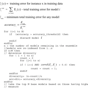
In this section we describe the DI classification algorithms and their regression vari-ants. DI consists of 3 techniques Dynamic Selection, Dynamic Voting and Dynamic Voting with Selection. We refer to their regression counterparts as Dynamic Selection, Dynamic Weighting and Dynamic Weighting with Selection. Dynamic Selection makes a localized selection of a model based on which model has the lowest cumula-tive error for the nearest neighbours to the test instance. The procedure for regression remains the same. Dynamic Voting assigns a weight to each base model based on its localized performance on the NN set and the final classification is based on weighted voting. Dynamic Weighting (DW) is similar to the Dynamic Voting in its calculation of weights but the final prediction is made by summing each of the base models pre-dictions weighted by a normalized weight value. Dynamic Weighting with Selection (DWS) is a regression derivative of Dynamic Voting with Selection. The process is similar to Dynamic Weighting except that base model with cumulative error in the upper half of the error interval,

E

i

>

(

E

max

−

E

min

) / 2

, (where

E

maxis the largest

cumulative error of any model and

E

minis the lowest cumulative error of any model ) are discarded from adding to the prediction.

members from the ensemble that are considered too inaccurate to be effective and then to consider the remaining members based on both their accuracy and diversity.

( ) training error for instance x in training data i

E x =

i Train

= E ( ) - total training error for model

sum i

x

E x i

∈

∑

min minimum total training error for any model

E −

min i sum i

E accuracy

E =

for (i=1 to N)

if (accuracyi > accuracy_threshold) then discard model

i

endif endfor

n = the number of models remaining in the ensemble //models are re-indexed from 1..n

if n>M then

// determine diversity for ( i = 1 to n)

count = 0 for (j=1 to n)

if ( i<>j AND ( , )

i j

correl E E > 0.6) then count = count + 1;

endif endfor

diversityi= (n–count)/n acc+divi = accuracy_i+diversityi

endfor

[image:4.595.130.418.180.477.2]

// take the top M base models based on those having highest acc+div_i // measure

Figure 1 Ensemble size reduction technique

3 Experimental Setup

which has been transformed to contain different random subsets of the variables. We chose the model tree technique M5, which combines instance based learning with regression trees [14] as the meta-model for SR. We chose this as it has a larger hy-pothesis space than simple linear regression. In the experiments where the ensemble

size was reduced the initial ensemble set had size

N

=

25 and was reduced to

10

M

=

with an accuracy_threshold of 0.66. Each of the DI techniques used

dis-tance weighted 5-NN as their meta-model.

4 Experimental Results

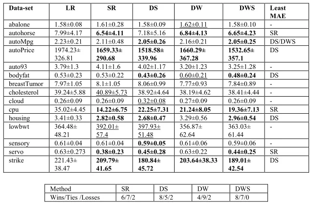
This section is divided into two sections where each section consists of two experi-ments; the first is related to the accuracy of the ensembles for the whole ensemble set; the second assesses the accuracy of the ensemble to the experiments when the ensem-bles are reduced in size. Each section consists of the results of the comparison with the base model of LR and 5-NN respectively. The results of each experiment over the 15 data-sets is presented in the form of a table where the first column gives the name of the data-set, the second column the base models’ MAE ± standard deviation for each data-set, and column 3-6 gives the MAE for each ensemble technique. The remaining column records the technique with the least MAE, if any of the techniques were able to significantly improve upon the performance of the base model, otherwise the entry is left blank. An ensemble MAE result which is significantly better than the base model is shown in bold, if it is significantly worse it is shown underlined. An adjunct

table summarizes the results of the significance comparison in the form of wins/

draws/losses where wins is the number of data-sets where the ensemble outperformed

the base model, draws is the number of data-sets for which the base model showed no

significant difference in accuracy to the base model, and losses is the number of

data-sets where the ensemble accuracy was worse than the base model.

4.1 Whole Ensemble set

Data-set LR SR DS DW DWS Least MAE abalone 1.58±0.08 1.61±0.28 1.58±0.09 1.62±0.11 1.58±0.10 - autohorse 7.99±4.17 6.54±4.11 7.18±5.16 6.84±4.13 6.65±4.23 SR autoMpg 2.23±0.21 2.11±0.48 2.05±0.26 2.16±0.21 2.05±0.25 DS/DWS autoPrice 1974.23±

326.81 1659.33± 290.68

1518.58± 339.96 1660.29± 367.28 1532.65± 357.1 DS auto93 3.79±1.3 4.11±1.6 4.02±1.17 3.20±1.23 3.25±1.28 - bodyfat 0.53±0.23 0.53±0.22 0.43±0.26 0.60±0.21 0.48±0.24 DS breastTumor 7.97±1.05 8.1±1.05 8.06±0.99 7.77±0.93 7.84±0.89 - cholesterol 39.24±5.88 40.89±5.73 38.92±4.64 38.19±4.62 38.41±4.44 - cloud 0.26±0.09 0.26±0.09 0.32±0.08 0.27±0.09 0.26±0.09 - cpu 35.02±4.45 14.22±6.75 22.25±7.31 21.24±8.05 19.36±7.13 SR housing 3.41±0.33 2.82±0.58 2.68±0.47 3.29±0.56 2.96±0.54 DS lowbwt 364.48±

48.21 392.01± 57.4 397.93± 51.48 356.87± 62.64 363.03± 61.44 - sensory 0.61±0.04 0.61±0.04 0.59±0.05 0.61±0.06 0.59±0.06 - servo 0.63±0.273 0.38±0.23 0.45±0.28 0.63±0.22 0.44±0.25 SR strike 221.43±

38.47 209.79± 41.65 180.84± 45.72 203.64±38.33 189.01± 42.54 DS

Method SR DS DW DWS

[image:6.595.138.457.156.364.2]

Wins/Ties /Losses 6/7/2 8/5/2 4/9/2 8/7/0

Table 1. The comparison of ensembles using LR as the base model

Data-set 5-NN SR DS DW DWS Least MAE

Abalone 1.61±0.09 1.54±0.08 1.73±0.07 1.54±0.09 1.54±0.09 SR/DW/DWS

autohorse 8.7±4.69 7.11±3.71 5.79±4.57 6.44±4.93 6.06±4.92 DS

autompg 2.31±0.38 2.12±0.34 2.41±0.35 2.04±0.35 2.08±0.35 DW

autoprice 1531.86± 404.24 1478.62± 460.89 1382.06± 336.79 1438.39± 460.48 1397.63± 454.43 DWS

auto93 3.81±1.4 3.76±1.11 4.27±1.32 3.4±1.52 3.39±1.58 DWS

bodyfat 2.3±0.49 0.94±0.21 1.16±0.28 1.7±0.37 1.407±0.34 SR

breastTumor 9.39±1.04 8.38±0.64 9.67±1.06 8.01±0.91 8.12±0.97 DW

cholesterol 43.0±4.13 43.39±4.03 46.17±6.04 39.64±4.63 40.36±4.56 DW

cloud 0.51±0.19 0.38±0.13 0.39±0.11 0.39±0.17 0.36±0.14 DWS

Cpu 22.72±13.94 34.16±17.61 23.97±12.97 19.68±13.46 20.72±14.18 DW

housing 2.59±0.58 2.30±0.41 2.56±0.39 2.39±0.55 2.27±0.5 DWS

lowbwt 398.3±80.6 397.8±47.17 471.35±

67.56 365.88± 80.53 369.47± 74.71

DWS

sensory 0.6±0.06 0.55±0.06 0.66±0.07 0.58±0.05 0.58±0.05 SR

servo 0.56±0.19 0.38±0.30 0.42±0.24 0.62±0.22 0.42±0.22 SR

strike 194.62± 53.46

222.29± 46.7

196.71±

50.16 182.25± 50.01 176.08± 50.15

DWS

Method SR DS DW DWS

[image:6.595.132.463.389.598.2]

Wins/ Draws/losses 9/3/3 4/7/4 13/2/0 13/2/0

Table 2. The comparison of ensembles using 5-NN as the base model

the error. DWS came first in rank order of the techniques which gave the least error most frequently with DW coming second.

In summary, it can be seen that for either base model, at least one of the DI techniques is as effective as SR, if not more so in reducing the error. Also DWS seemed to be the most reliable ensemble approach, as it never significantly increased the error. The pattern of behaviour of the DI techniques for regression mirrors that of classification [16] where the best integration method varied with the data-set and the base model.

4.2 Reduced Ensemble set

In this section, we repeated the experiments of the previous section, but with the addi-tion that the ensemble set had been reduced at the end of the training phase using the

algorithm described in Figure 1 from

N

=

25

to

M

=

10

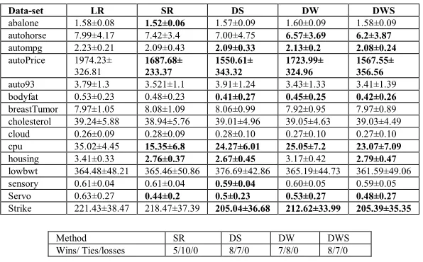
. Table 3 shows the results

of the comparison of the reduced size ensembles for LR. Comparing the ties/wins/losses of Table 3 to Table 1 shows that DW and DS improved in perform-ance, DWS remained the same and SR remained approximately the same.

Data-set LR SR DS DW DWS abalone 1.58±0.08 1.52±0.06 1.57±0.09 1.60±0.09 1.58±0.09 autohorse 7.99±4.17 7.42±3.4 7.00±4.75 6.57±3.69 6.2±3.87 autompg 2.23±0.21 2.09±0.43 2.09±0.33 2.13±0.2 2.08±0.24 autoPrice 1974.23±

326.81 1687.68± 233.37 1550.61± 343.32 1723.99± 324.96 1567.55± 356.56 auto93 3.79±1.3 3.521±1.1 3.91±1.24 3.43±1.33 3.41±1.39 bodyfat 0.53±0.23 0.48±0.23 0.41±0.27 0.45±0.25 0.42±0.26 breastTumor 7.97±1.05 8.08±1.09 8.06±0.99 7.92±0.95 7.97±0.89 cholesterol 39.24±5.88 38.94±5.76 39.01±4.96 39.05±4.63 39.03±4.49 cloud 0.26±0.09 0.28±0.09 0.28±0.10 0.27±0.10 0.27±0.10 cpu 35.02±4.45 15.35±6.8 24.27±6.01 25.05±7.2 23.07±7.09 housing 3.41±0.33 2.76±0.37 2.67±0.45 3.17±0.42 2.79±0.47 lowbwt 364.48±48.21 365.46±50.86 376.69±42.86 365.19±44.73 361.59±49.06 sensory 0.61±0.04 0.61±0.04 0.59±0.04 0.60±0.05 0.59±0.05 Servo 0.63±0.27 0.44±0.2 0.5±0.23 0.53±0.27 0.48±0.27 Strike 221.43±38.47 218.47±37.39 205.04±36.68 212.62±33.99 205.39±35.35

Method SR DS DW DWS

[image:7.595.150.448.368.553.2]

Wins/ Ties/losses 5/10/0 8/7/0 7/8/0 8/7/0

Table 3. Results of comparison of ensembles using LR

There is however more variation in the results than the summary in significance comparison alone would suggest. If we calculate the percentage change in MAE be-tween the results in Table 1 and Table 3 and average it over all data-sets, the follow-ing average percentage changes are shown in Table 4. A positive value is recorded if the technique gave on average a percentage reduction in error.

Technique SR DS DW DWS Average percentage change in

MAE

[image:8.595.142.453.169.202.2]

-0.45±8.3 -0.72±6.36 0.9±9.89 -1.41±7.41

Table 4. Percentage change in MAE for ensemble size from N to M

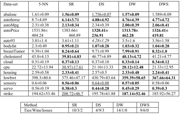
However comparing the reduced ensemble set to the whole ensemble results in detail shows a general trend that for data-sets where the error increased it did not increase to change the level of significance, but where the error decreased then in some cases it did change the signifcance comparison. e.g. consider the technique DW , for the whole ensemble set, autohorse, autoprice, cpu, strike gave an MAE better than the base model whereas abalone, and bodyfat were significantly worse. For the reduced ensemble set, autohorse, autompg, autoprice, bodyfat, cpu, servo, strike gave an MAE significantly better than base model even though for some of these data-sets there was a relative increase in MAE.

Data-set 5-NN SR DS DW DWS

abalone 1.61±0.09 1.56±0.09 1.756±0.07 1.57±0.09 1.589±0.09 autohorse 8.7±4.69 6.14±3.71 4.88±4.92 4.76±4.39 4.77±4.72 autoMpg 2.31±0.38 2.13±0.34 2.34±0.39 2.00±0.39 2.06±0.41 autoPrice 1531.86±

404.24 1383.66± 460.89 1320.41± 236.91 1313.78± 462.28 1326.41± 419.81 auto93 3.81±1.4 3.61±1.11 4.28±1.29 3.5±1.6 3.56±1.58 bodyfat 2.3±0.49 0.95±0.21 1.07±0.28 1.03±0.32 1.04±0.28 breastTumor 9.39±1.04 8.24±0.64 9.71±0.99 7.99±0.91 8.32±1.0 cholesterol 43.0±4.13 39.81±4.03 46.77±6.89 40.13±4.72 41.21±4.77 cloud 0.51±0.19 0.37±0.13 0.37±0.10 0.33±0.14 0.34±0.12 cpu 22.72±13.94 30.97±17.61 21.10±13.33 20.12±12.48 21.33±12.95 housing 2.59±0.58 2.33±0.41 2.57±0.5 2.33±0.48 2.24±0.41 lowbwt 398.3±80.6 375.46±47.17 430.79±83.64 359.39±58.65 367.66±64.31 sensory 0.6±0.06 0.56±0.06 0.64±0.08 0.57±0.05 0.58±0.06 servo 0.56±0.19 0.38±0.3 0.44±0.28 0.45±0.29 0.39±0.3 strike 194.62±53.46 208.72±46.7 195.78±61.88 187.14±52.46 185.92±56.27

Method SR DS DW DWS

[image:8.595.150.447.345.535.2]

Ties/Wins/losses 10/3/2 4/9/3 14/1/0 9/6/0

Table 5 Comparison of Ensembles with the base model 5-NN

was a positive change in the average percentage change in error, with a relatively large change for DW.

Technique SR DS DW DWS Average percentage change in

MAE

[image:9.595.131.458.181.213.2]

3.49±4.69 3.53±5.61 7.42±13.23 3.04+9.12

Table 6 Percentage change in MAE for ensemble size = N to M

In summary, the ensemble size reduction strategy maintains the effective-ness both of SR and the DI techniques. In the case DW, the results would suggest that in fact pruning the ensemble set actually improves accuracy, a likely consequence that it is more sensitive to in-accurate or redundant base models, than the DS and DWS approaches, which either select the best model or remove inaccurate models from the model combination.

5 Conclusions and Future Work

In this paper we have demonstrated that the classification ensemble techniques of Dynamic Integration can be adapted to the problem of regression. We have shown that for simple base models, these techniques are as effective as Stacked Regression for the range of data-sets tested. We have presented a extension to the SR and DI techniques which uses the accuracy and diversity measure captured in the training of the base models to prune the size of the ensemble thus removing models that are ineffective in the model combination. We intend to refine and improve on this simple technique as it provides little extra overhead to the algorithms and has shown promising results in reducing the ensemble size whilst maintaining its level of accuracy. In particular, we intend to investigate in more detail the appropriate choice of accuracy threshold and the size of the reduced ensemble set. Also, we shall compare our measure for diversity to the more commonly known measures for diversity such as the variance based measure developed in [8].

6 Acknowledgements

We gratefully acknowledge the WEKA framework [16] within which the ensemble methods were implemented and assessed. Dr Tsymbal acknowledges Science Founda-tion, Ireland.

References

2. Christensen, S. 2003. Ensemble Construction via Designed Output Distortion In Proc. 4th _{International Workshop on Multiple Classifier Systems, LNCS,} Vol. 2709, pp. 286-295, Springer-Verlag.

3. Dietterich, T. 2000. Ensemble Methods in Machine Learning, In Proc. 1st

International Workshop on Multiple Classifer Systems, LNCS, Vol 1857, pp. 1-10, Springer-Verlag.

4. Giacinto, G. and Roli, F. 2000. Dynamic Classifier Selection, In Proc. 1st

Int. Workshop on Multiple Classifier Systems, LNCS, Vol 1857, pp. 177-189, Springer-Verlag.

5. Ho, T. K. 1998a. The random subspace method for constructing decision

for-ests. IEEE PAMI, 20(8):832--844.

6. Ho, T.K. 1998b. Nearest Neighbors in Random Subspaces, LNCS: Advances

in Pattern Recognition, 640-648.

7. Kleinberg, E.M. 1990. Stochastic Discrimination, Annals of Mathematics

and Artificial intelligence, 1:207-239.

8. Krogh, A. and Vedelsby, J. 1995. Neural Networks Ensembles, Cross

valida-tion, and Active Learning, Advances in Neutal Information Processing

Sys-tems, MIT Press, pp. 231-238.

9. Kuncheva L.I. 2002. Switching between selection and fusion in combining

classifiers: An experiment, IEEE Transactions on SMC, Part B, 32 (2),,

146-156.

10. LeBlanc, M. and Tibshirani, R. 1992. Combining estimates in Regression

and Classification, Technical Report, Dept. of Statistics, University of To-ronto.

11. Merz, C.J. 1996. Dynamical selection of learning algorithms. In Learning

from data, artificial intelligence and statistics. .Fisher and H.-J.Lenz (Eds.) New York: Springer.

12. Merz, C. and Pazzani, M. 1999. A principal components approach to

com-bining regression estimates, Machine Learning, 36:9-32.

13. Puuronen, S., Terziyan, V., Tsymbal, A. 1999. A Dynamic Integration

Algo-rithm for an Ensemble of Classifiers.Foundations of Intelligent Systems,

11th International Symposium ISMIS’99, LNAI, Vol. 1609: 592-600, Springer-Verlag.

14. Quinlan, R. 1992. Learning with continuous classes, In Proceedings of the 5th

Australian Joint Conference on Artificial Intelligence, World Scientific, pp. 343-348.

15. Schaffer, C. 1993. Overfitting avoidance as bias. Machine Learning

10:153-178.

16. Sharkey, A.J C. (Ed.) 1999. Combining Artificial Neural Nets: Ensemble and

Modular Multi-Net Systems. Springer-Verlag,.

17. Tsymbal, A., Puuronen, S., Patterson, D. 2003. Ensemble feature selection

with the simple Bayesian classification, Information Fusion Vol. 4:87-100,

Elsevier.

18. Witten, I. and Frank, E. 1999. Data Mining: Practical Machine Learning

Tools and Techniques with Java Implementations, Morgan Kaufmann.